The document discusses back-propagation networks in neural networks, detailing their structure, learning rules, and weight adjustments. It highlights the significance of hidden layers for improved expressiveness, generalization, and tolerance to noise, despite challenges in computational efficiency and transparency. The learning process involves measuring and reducing error through gradient descent techniques.

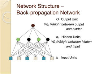
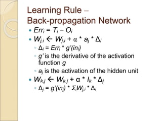
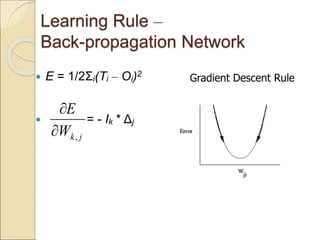
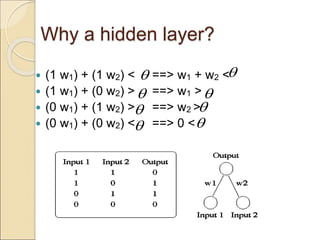
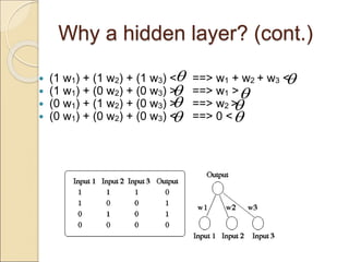
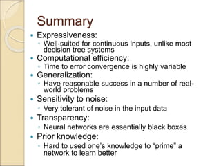
1. Back-Propagation
C.Eben Exceline,
AP/AI&DS,
Excel Engineering
College

2. Network Structure –
Perceptron
O Output Unit
Wj Weight
Ij Input Units

3. Network Structure –
Back-propagation Network
Oi Output Unit
Wj,I Weight between output
and hidden
aj Hidden Units
Wk,j Weight between hidden
and Input
Ik Input Units

4. Learning Rule
 Measure error (sum of mean square
error)
 Reduce that error
◦ By appropriately adjusting each of the
weights in the network

5. Learning Rule –
Perceptron
 Err = T – O
◦ O is the predicted output
◦ T is the correct output
 Wj  Wj + α * Ij * Err
◦ Ij is the activation of a unit j in the input
layer
◦ α is a constant called the learning rate

6. Learning Rule –
Back-propagation Network
 Erri = Ti – Oi
 Wj,i  Wj,i + α * aj * Δi
◦ Δi = Erri * g’(ini)
◦ g’ is the derivative of the activation
function g
◦ aj is the activation of the hidden unit
 Wk,j  Wk,j + α * Ik * Δj
◦ Δj = g’(inj) * ΣiWj,i * Δi

7. Learning Rule –
Back-propagation Network
 E = 1/2Σi(Ti – Oi)2
 = - Ik * Δj
j
k
W
E
,


Gradient Descent Rule

8. Why a hidden layer?
 (1 w1) + (1 w2) < ==> w1 + w2 <
 (1 w1) + (0 w2) > ==> w1 >
 (0 w1) + (1 w2) > ==> w2 >
 (0 w1) + (0 w2) < ==> 0 <



 




9. Why a hidden layer? (cont.)
 (1 w1) + (1 w2) + (1 w3) < ==> w1 + w2 + w3 <
 (1 w1) + (0 w2) + (0 w3) > ==> w1 >
 (0 w1) + (1 w2) + (0 w3) > ==> w2 >
 (0 w1) + (0 w2) + (0 w3) < ==> 0 <









10. Summary
 Expressiveness:
◦ Well-suited for continuous inputs, unlike most
decision tree systems
 Computational efficiency:
◦ Time to error convergence is highly variable
 Generalization:
◦ Have reasonable success in a number of real-
world problems
 Sensitivity to noise:
◦ Very tolerant of noise in the input data
 Transparency:
◦ Neural networks are essentially black boxes
 Prior knowledge:
◦ Hard to used one’s knowledge to “prime” a
network to learn better

11. Conclusions (cont.)