This paper presents a novel method for autonomous traffic signal control using decision trees to optimize signal durations and reduce traffic congestion. By employing real-time vehicle counting through image processing techniques, the system dynamically adjusts traffic signals based on vehicle presence at each lane of a junction. The decision-making process employs a structured algorithm that assesses the vehicle counts and adjusts signal statuses to enhance traffic flow and minimize delays.

1. International Journal of Electrical and Computer Engineering (IJECE)
Vol. 8, No. 3, June 2018, pp. 1522~1529
ISSN: 2088-8708, DOI: 10.11591/ijece.v8i3.pp1522-1529  1522
Journal homepage: http://iaescore.com/journals/index.php/IJECE
Autonomous Traffic Signal Control using Decision Tree
Rithesh R. N., Vignesh R, Anala M. R.
R V College of Engineering, Bangalore, Indonesia
Article Info ABSTRACT
Article history:
Received Oct 17, 2017
Revised Dec 26, 2017
Accepted Jan 3, 2018
The objective of this paper is to introduce an effective and efficient way of
traffic signal light control to optimize the traffic signal duration across each
lanes and thereby, to minimize or completely eliminate traffic congestion.
This paper introduces a new approach to resolve the traffic congestion
problem at junctions by making use of decision trees. The vehicle count in
the real time traffic video is determined by Image Processing technique. This
information is fed to the decision tree based on which the decision is made
regarding the status of traffic signal lights of each lane at the junction at any
given instant of time.
Keyword:
Background subtraction
Decision tree
Object detection
Traffic congestion
Vehicle count Copyright © 2018 Institute of Advanced Engineering and Science.
All rights reserved.
Corresponding Author:
Anala M. R.,
Departement of Computer Science and Engineering,
R V College of Engineering,
R.V. Vidyaniketan Post, Mysuru Road, Bengaluru – 560059, India.
Email : analamr@rvce.edu.in
1. INTRODUCTION
The primary intension of the traffic signal lights is to facilitate the transportation or movement of the
vehicles in junctions without creating any chaos or adversely affecting the normal day to day life of people.
Efficient working of the same is an essential part for smooth transportation, especially in densely populated
metropolitan cities. But in today‟s age of globalization the number of vehicles stepping onto the road has
elevated by significant amount leading to traffic congestion problem. Traffic congestion has emerged as one
of the most serious problems faced by most of the countries today. It has adverse effect on the physical and
mental health of the people, the environment, and is one of the main reasons for the cause of accidents. All of
these problems can be minimized and in some cases completely eliminated by incorporating the right
methodology which controls and coordinates flow of vehicles on the road in an efficient manner, and thereby
makes optimum utilization of time and available space for vehicle transportation. This paper introduces an
efficient way for traffic signal light control using decision trees. The decision tree modeled here is mainly
based on the number of vehicles on each lane at the junction. The count of the number of vehicles across
each lane at the junction is obtained by using Image processing techniques. The decision regarding the status
(i.e. color) of the signal lights across each lanes of the junctions is made based on the number of vehicles on
each lanes and, accordingly the status of the signal lights are changed in real time to achieve maximum
throughput in terms of number of vehicles clearing/crossing the junction, with minimum chances of traffic
jam.
2. LITERATURE REVIEW
Intelligent transportation systems (ITS) mainly aim at providing better quality of traffic congestion
control.

2. Int J Elec & Comp Eng ISSN: 2088-8708 
Autonomous Traffic Signal Control using Decision Tree (Anala M. R.)
1523
The world has seen huge advancements in ITS some of them are follows:
A methodology in which the system detects and controls the traffic congestion in real time based on
the extent to which congestion has occurred by employing active RFID (gateway, router and tags) and GSM
technology is discussed in [1]. This method requires each vehicles to have RFID tag installed in them and
based on the relative speeds of the vehicles the traffic signal is controlled by the coordinators. This technique
requires a huge initial investment for system setup and, difficult to implement in cities with high congestion
problem because the traffic congestion at given signal not only affects the signal lights of this junction but
also influences the signal lights of previous junctions. Therefore due to chain reaction, in the worst case a
series of signals can experience a severe congestion problem.
The technique in which traffic signal control is done using image processing techniques is presented
in [2]-[4]. The similarity between a reference image of a road and the real image of same road becomes the
criteria for traffic signal light control. Higher the similarity lower is the number of vehicles and viz.
Preference is given to road which has least similarity value. This technique takes into account only the
similarity value therefore irrespective of number of vehicles across each lanes GREEN signal is given to only
those lanes with least similarity value. There might occur a situation in which one lane has fewer number of
Large Motor Vehicles(LMV) in which the similarity value is small and another lane might have greater
number of small sized vehicles covering less area across the road compared to the road with LMV thus
similarity value would be comparatively high. In this case former lane is given GREEN signal and later case
is given RED signal thus failing to avoid congestion at the densely populated roads.
A methodology in which the vehicle count is determined using Image processing technique and a
learning model is designed which predicts the duration of traffic signal for the next iteration based on the
available data of current iteration, is presented in [5]. Also, [6] and [7] proposes alternative techniques to
overcome traffic congestion and traffic accidents.
3. RESEARCH METHOD
The proposed methodology encompasses two main phases:
a. Object detection and vehicle counting
b. Decision making using Decision tree.
Each of these phases is explained in detail in the following section.
3.1. Object detection and vehicle counting
A camera capable of capturing all the lanes at a given junction has to be setup. The position and
orientation of this camera should be consistent in giving the proper view of all the lanes. A balanced pictorial
view of all the lanes obtained from the camera helps in achieving better results for decision making process.
This real time video from this camera is given as input to the microcontroller/microprocessor. The Image
processing technique for object detection and counting and, the algorithm for decision making is
programmed in the microprocessor. The image processing technique used here follows extraction of frames
from the video, Background subtraction, threshold setup, creating contours, blob detection, and vehicle
counting which is more accurate than the object detection technique presented in [8] and [9]. The captured
video is broken down into sequence of frames, the frames are extracted at a rate of 25 frames/sec. These
sequences of frames are processed to detect multiple moving objects (vehicles). For the purpose of
explanation, the algorithm is applied for a two lane traffic junction. At the beginning of this algorithm the
vehicle count across all the lanes is initialized to zero. A virtual line is drawn across each lanes at the junction
to keep track on the number of vehicles waiting to cross the junction. The virtual lines are considered as the
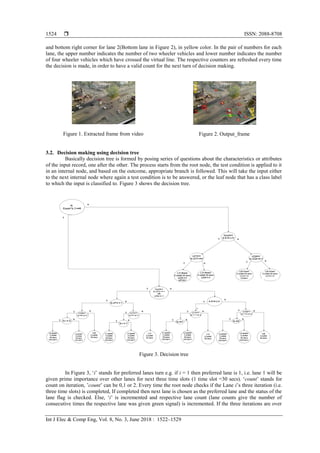
line of reference for the movement of the vehicles. Figure 1 shows original image extracted from the video
and the image with virtual lines draws across each of the lanes of the junction.
The extracted frames from the video are converted into binary black and white image. It is evident
from [10] that Canny Edge detection is the most efficient technique for object edge extraction, hence the
same technique is used here. Contours are drawn for the binary image and convex hulls are constructed with
the help of these contours and, finally blobs are formed. Each of valid blobs are added to the list list_blobs.
For each and every blob in the list list_blobs, if the blob has crossed the virtual line then the vehicle counter
associated with the corresponding lane is incremented. The blobs may be categorized as 2-wheeler or 4-
wheeler based on the size and aspect ratio. And also two separate counters may be assigned to each lane at
the junction, one to account for number of two wheeler vehicles waiting to cross the junction and the other
for four wheeler. Crossing the line merely refers to the fact that the midpoint of the blob under reference is on
one side of the line in the previous frame and in the current frame the midpoint is on or has crossed the
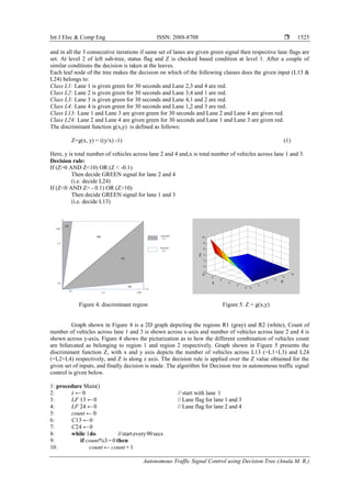
virtual line. In Figure 2 for each of the lanes two counters are maintained respectively. One for the 2 wheeler
vehicle and the other for the 4 wheeler vehicle as shown in the top left corner for lane 1(Left lane in Figure 2)

3.  ISSN: 2088-8708
Int J Elec & Comp Eng, Vol. 8, No. 3, June 2018 : 1522–1529
1524
and bottom right corner for lane 2(Bottom lane in Figure 2), in yellow color. In the pair of numbers for each
lane, the upper number indicates the number of two wheeler vehicles and lower number indicates the number
of four wheeler vehicles which have crossed the virtual line. The respective counters are refreshed every time
the decision is made, in order to have a valid count for the next turn of decision making.
Figure 1. Extracted frame from video Figure 2. Output_frame
3.2. Decision making using decision tree
Basically decision tree is formed by posing series of questions about the characteristics or attributes
of the input record, one after the other. The process starts from the root node, the test condition is applied to it
in an internal node, and based on the outcome, appropriate branch is followed. This will take the input either
to the next internal node where again a test condition is to be answered, or the leaf node that has a class label
to which the input is classified to. Figure 3 shows the decision tree.
Figure 3. Decision tree
In Figure 3, „i‟ stands for preferred lanes turn e.g. if i = 1 then preferred lane is 1, i.e. lane 1 will be
given prime importance over other lanes for next three time slots (1 time slot =30 secs). „count‟ stands for
count on iteration, ‟count‟ can be 0,1 or 2. Every time the root node checks if the Lane i‟s three iteration (i.e.
three time slots) is completed, If completed then next lane is chosen as the preferred lane and the status of the
lane flag is checked. Else, „i‟ is incremented and respective lane count (lane counts give the number of
consecutive times the respective lane was given green signal) is incremented. If the three iterations are over

4. Int J Elec & Comp Eng ISSN: 2088-8708 
Autonomous Traffic Signal Control using Decision Tree (Anala M. R.)
1525
and in all the 3 consecutive iterations if same set of lanes are given green signal then respective lane flags are
set. At level 2 of left sub-tree, status flag and Z is checked based condition at level 1. After a couple of
similar conditions the decision is taken at the leaves.
Each leaf node of the tree makes the decision on which of the following classes does the given input (L13 &
L24) belongs to:
Class L1: Lane 1 is given green for 30 seconds and Lane 2,3 and 4 are red.
Class L2: Lane 2 is given green for 30 seconds and Lane 3,4 and 1 are red.
Class L3: Lane 3 is given green for 30 seconds and Lane 4,1 and 2 are red.
Class L4: Lane 4 is given green for 30 seconds and Lane 1,2 and 3 are red.
Class L13: Lane 1 and Lane 3 are given green for 30 seconds and Lane 2 and Lane 4 are given red.
Class L24: Lane 2 and Lane 4 are given green for 30 seconds and Lane 1 and Lane 3 are given red.
The discriminant function g(x,y) is defined as follows:
Z=g(x, y) = ((y/x) -1) (1)
Here, y is total number of vehicles across lane 2 and 4 and,x is total number of vehicles across lane 1 and 3.
Decision rule:
If (Z>0 AND Z<10) OR (Z < -0.1)
Then decide GREEN signal for lane 2 and 4
(i.e. decide L24)
If (Z<0 AND Z> - 0.1) OR (Z>10)
Then decide GREEN signal for lane 1 and 3
(i.e. decide L13)
Figure 4. discriminant region Figure 5. Z = g(x,y)
Graph shown in Figure 4 is a 2D graph depicting the regions R1 (gray) and R2 (white), Count of
number of vehicles across lane 1 and 3 is shown across x-axis and number of vehicles across lane 2 and 4 is
shown across y-axis, Figure 4 shows the picturization as to how the different combination of vehicles count
are bifurcated as belonging to region 1 and region 2 respectively. Graph shown in Figure 5 presents the
discriminant function Z, with x and y axis depicts the number of vehicles across L13 (=L1+L3) and L24
(=L2+L4) respectively, and Z is along z axis. The decision rule is applied over the Z value obtained for the
given set of inputs, and finally decision is made. The algorithm for Decision tree in autonomous traffic signal
control is given below.
1: procedure Main()
2: i ← 0 // start with lane 1
3: LF 13 ←0 // Lane flag for lane 1 and 3
4: LF 24 ←0 // Lane flag for lane 2 and 4
5: count ← 0
6: C13 ←0
7: C24 ←0
8: while 1do //startevery90secs
9: if count%3=0 then
10: count ← count + 1

5.  ISSN: 2088-8708
Int J Elec & Comp Eng, Vol. 8, No. 3, June 2018 : 1522–1529
1526
11: if LF13 = 1 || LF24 = 1 then
12: if LF 13 = 1 then // L13 wasgreenfor last90secs
13: LF13 = 0
14: C24 ← C24 +1
15: START_WITH_L24
16: else //L24 wasgreen for last90secs
17: LF24 = 0
18: C13 ← C13 +1
19: START_WITH_L13
20: endif
21: else
22: if Determine_G = L24 then //L24hasmorevehicles
23: C24 ← C24 +1
24: START_WITH_L24
25: else //L13hasmorevehicles
26: C13 ← C13 +1
27: START_WITH_L13
28: endif
29: endif
30: else
31: count ← count + 1
32: if DETERMINE_G=L13 then
33: Lane1 ← Lane3 ←green
34: C13 ← C13 +1
35: C24 =0
36: outlet ← 2
37: wait30secs
38: if C13 = 3 then
39: LF13 = 1
40: endif
41: else
42: Lane2 ← Lane4 ←green
43: C24 ← C24 +1
44: C13 ←0
45: outlet ← 2
46: wait30secs
47: if C24 = 3 then
48: LF24 = 1
49: endif
50: endif
51: endif
52: end while
53: endprocedure
54: procedure Determine_G()
55: LC24 ← LC2 + LC4
56: LC13 ← LC1 + LC3
57: G←LC24/LC13−1
58: if G > 0&& G < 10then returnL24
59: else return L13
60: endif
61: endprocedure
62: procedure START_WITH_L24()
63: if i = 2 then
64: Lane2 ←green
65: Outlet ← 3
66: else if i= 4 then
67: Lane4 ←green
68: Outlet ← 3
69: else

6. Int J Elec & Comp Eng ISSN: 2088-8708 
Autonomous Traffic Signal Control using Decision Tree (Anala M. R.)
1527
70: Lane2 ← Lane4 ←green
71: Outlet ← 2
72: wait30secs
73: endif
74: endprocedure
75: procedure START_WITH_L13()
76: if i = 1 then
77: Lane1 ←green
78: Outlet ← 3
79: else if i= 3 then
80: Lane3 ←green
81: Outlet ← 3
82: else
83: Lane1 ← Lane3 ←green
84: Outlet ← 2
85: wait30secs
86: endif
87: endprocedure
In this context, the input to the decision tree are the features of 4 lanes L1, L2, L3 and L4. These
features include the vehicle count of each lane and a flag associated with the pair of lanes i.e. LF13 and
LF24.The flag value 1 for a pair of lanes specifies that they were given green signal for 3 consecutive time
(30 sec each). The leaf nodes specifies which lanes should be given with the green signal for the next 30 secs
and also marks the flags of the lanes if they were given green signals for 3 consecutive times which is used as
the input to the next iteration.
Figure 6. 3 outlet format and 2 outlet format
3 outlet format: In this format, a selected lane (say L1) allows its vehicles to move in 3 directions i.e
straight (along lane3), left (along lane2) and right (along lane4).
2 outlet format: In this format, a selected lane (say L1) allows its vehicles to move in 2 directions i.e
straight (along lane3) and left (along lane2). Figure 6 represents both these formats.
The tree is executed once in every time slot (30 secs). First we check if 90 seconds (i.e three 30sec
time slots) is completed using the condition count%3 =0. if it has then we check if any pair of lanes (L13 or
L24) were given green signal for 90 secs i.e. for 3 continuous slots. If that‟s true (say L13 was green for 90
secs), then irrespective of the result of the Z function, the other two lanes (i.e. L24) are given the preference
so as to avoid starvation. If none of the flags were set, the function Z is called to decide which of the pairs is
to be given preference for the first 30 secs (Assume Z decides L24). So for the first 30 secs, one of these two
lanes (L2 or L4) has to be given green signal with 3 outlet format, based on „i‟ value. The lane which has its
turn in this iteration is selected here. ie, if L2 is preferred lane in this iteration then L2 is selected or if L4 has
its turn then L4 is selected. If neither of them had its turn, i.e L1 or L3 had its turn in the corresponding
iteration, but based on Z L24 got green then both of them are given green with 2 outlet format. In the second
and third time slots only 2 outlet format is followed based on pair of lanes chosen by Z. If count % 3 is not 0,
i.e. 90 secs is not completed, then the pair of lanes is selected purely based on the result of function Z. Here is
where we check if a pair is being given green signal for 3 consecutive times or 90 consecutive seconds and
thereby set the corresponding flags to avoid starvation of the other pair of lanes. For a 4 lane structure of the
decision tree, the following methodology is followed:

7.  ISSN: 2088-8708
Int J Elec & Comp Eng, Vol. 8, No. 3, June 2018 : 1522–1529
1528
For every iteration (i.e every 30 secs) L13 (= L1 + L3) and L24 ( = L2+L4) is computed. Every lane
(In this case 4 lanes) meeting at the junction is given equal priority in Round Robin fashion, i.e every lane
becomes preferred lane (gets 3 outlet format for 1st 30secs) within a maximum of 11 time slots and
irrespective of the magnitude of congestion at the traffic junction every lane get green signal (2 outlet format)
within a maximum of 6 time slots. After every 3 iterations, a lane „i‟ becomes preferred lane based on the
following rule
i = (i % 4) + 1 (2)
4. RESULTS AND ANALYSIS
The algorithm is implemented in C++ in visual studio along with openCV open source software.
The vehicle detection and counting algorithm was executed for 2 simulation videos and 3 real time videos,
each for a span of 60 seconds and the following results were obtained. Actual count column in the Table.1
signifies the actual number of vehicles in the video this count was obtained by manually counting the
vehicles. Count obtained column gives the number of moving vehicles identified by the algorithm, the
corresponding deviation and accuracy is mentioned in the Table 1. The implementation of this technique
consists of two different programs running simultaneously, one program constitutes the image processing
technique for moving vehicle detection and counting and, the other program is for making decision on status
of traffic signal light based on decision tree. The output of the former program is written in text file (input)
and the later program which is running simultaneously reads this text file (input) and makes decision on
traffic signal.
The output of the later program can be written to another text file or can be fed to control switches
of traffic lights. The model designed here is for the autonomous traffic control, thus the number of vehicles
across each of the lanes is determined and instantaneously written to the text file .This file is read
continuously by decision tree and correspondingly the status of the traffic lights is varied based on the real
time situation of the junction.
Table 1. Result Analysis
Sl. no Actual count Count obtained Deviation Accuracy Nature of video
1 52 52 0% 100% Real
2 118 92 22% 78% Real
3 72 72 0% 100% Simulation
4 51 60 17.50% 82.50% Simulation
5 109 106 0.02% 99.98% Real
The accuracy of the result is mainly dominated by quality of the video and the camera orientation.
The variation or difference between the actual vehicle count and the vehicle count obtained in traffic video is
attributed to the following factors:
a. Noise in the video- because of which most of the information is inconsistent and object detection
becomes more difficult. Applying denoising algorithm to each frame in the video tends to be time
consuming and results in loss of useful information.
b. Distance factor- when the group of vehicles are very close, the algorithm considers it as one single object
and thus the counting cannot be made 100% accurate.
c. Quality of the video
d. Placement/Position of the camera with respect to the cross road/junction.
Table 2. Decision Tree Results
Time
stamp(TS)
Lane1
(vehicle count)
Lane2
(vehicle count)
Decision Output
30 100 50 L1 L1 green for 30 secs
60 120 70 L1 L1 green for 30 secs
90 110 80 L1 L1 green for 30 secs
120 135 85 L2 L2 green for 30 secs
150 140 10 L1 L1 green for 30 secs
180 30 20 L1 L1 green for 10 secs
210 5 15 L2 L2 green for 30 secs
240 10 105 L1 L1 green for 30 secs

8. Int J Elec & Comp Eng ISSN: 2088-8708 
Autonomous Traffic Signal Control using Decision Tree (Anala M. R.)
1529
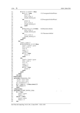
Table 2 describes the result of decision tree for a junction with 2 lanes. Lane 1 is given green signal
thrice each with time slot of 30 seconds. In the next turn even if L1 has more number of vehicle than L2, still
L2 is set to green thereby avoiding starvation. At time stamp 240 though L2 has more vehicles than L1 still
L1 is given green signal in order to avoid small number of vehicles waiting for a relatively longer duration of
time.
5. CONCLUSION
The model designed for autonomous traffic signal control is coherent with its purpose. The
methodology implemented here is completely based on number of vehicles across each lanes and, since
traffic congestion directly depends on number of vehicles waiting to cross junction across each lane. This
technique minimizes the traffic congestion, and in some cases it is completely eliminated. The statistics on
the vehicle count can also be used for the infrastructural development such as flyovers, metro etc. The
decision tree designed is a generic model and can be extended to any number of lanes by making appropriate
changes in different levels of the decision tree. The worst case scenario is when a set of vehicles of a lane has
to wait for 5 continuous slots or 150 secs. This seems highly impractical in reality. People can‟t know when
exactly they will be allowed to move as the decision is taken at run time at the end of 30 secs or a slot.
REFERENCES
[1] Siuli Roy, Somprakash Bandyopadhyay, Munmun Das, Suvadip Batabyal, Sankhadeep Pal, “Real Time Traffic
Congestion Detection and Management using Active RFID and GSM Technology”, In proc. of the 10th
International Conference on Intelligent Transport Systems Telecommunication (ITST’10).
[2] Nilay Mokashi, “Intelligent Traffic Signal Control using Image Processing”, International Journal of Advanced
Research in Computer Science and Management Studies, vol. 3, no. 10, 2015, ISSN: 2321-7782.
[3] Susmita A.Meshram, A.V. Malviya, “Traffic Surveillance by Counting and Classification of vehiclesfrom video
using Image processing”, International Journal of Advanced Research in Computer Science and Management
Studies, vol. 1, no. 6, 2013, ISSN: 2321-7782.
[4] Ms. Pallavi choudekar, Ms.b Sayanti Banerjee, Prof M.K. Muju, “Real time traffic light control using image
processing”, Indian Journal of Computer Science and Engineering, vol. 2, no. 1, ISSN: 0976-5166, pp. 6-10.
[5] Archit Peshave, Shantanu RajeNimbalkar, Ajinkya Puar, Vikas Gardare, Abhijeet Dodake, Jitendra Waydande,
“A Review on Autonomous Traffic Lights Control System”, International Journal of Innovative Research in
Computer and Communication Engineering, vol. 3, no. 10, October 2015, pp. 10034-10037.
[6] Sutikno, Helmie Arif Wibawa, Prima Yusuf Budiarto, “Classification of Road damage from digital Image using
Backpropagation Neural Network”, IAES International Journal of Artificial Intelligence, vol. 6, no. 4,
December 2017, ISSN: 2252-8938.
[7] Kusuma Kumari, Sampada Sethi, Ramakanth Kumar, Nishant Kumar, Atulit Shankar, “Driver Drowsiness
Detection System using Sensors”, IAES International Journal of Informatics and Communication Technology,
vol. 6, no. 3.
[8] Varun Sharma, “Object Counting using MATLAB”, International Journal of Scientific & Engineering Research,
vol. 5, no. 3, March 2014. ISSN 2229-5518.
[9] Ganesh Raghtate, Abhilasha K Tiwari, “Moving Object Counting in Video Signal”, International Journal of
Engineering Research and General Science, vol. 2, no. 3, 2014, ISSN: 2091-2730.
[10] Brinda R.B, Namratha Venkatesh Murthy, B.M. Ramya, Dr. Vijaya Prakash A M, “Edge detection Smart Traffic
Control”, International Journal of Innovative Research in Electrical, Electronics, Instrumentation and Control
Engineering, vol. 3, no. 11, 2015, ISSN: 2321-2004.