Large-scale Logging Made Easy: Meetup at Deutsche Bank 2024
Graphs
1. Graphs
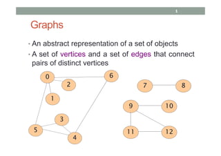
• An abstract representation of a set of objects
• A set of vertices and a set of edges that connect
pairs of distinct vertices
0000
1111
2222
6666
5555
3333
4444
7777 8888
9999 10101010
11111111 12121212
1
3. Solution to the Man-Wolf-Goat-Cabbage Problem
MWG
C-∅
WC-
MG
MWC-
G
C-
MWG
W-
MGC
MGC-
W
MWG-
C
∅-
MWGC
MG-
WC
G-
MWC
g
g
g
g
g g g g
m
m
m
m
w
w
w
w
c
c
c
c
3
5. Network Topology
• Describing how computers, printers, and other
devices are connected over a network.
• Describes the layout of wires, devices and
routing paths.
5
6. Game Representation – Tic Tac Toe
• Once the game is viewed
as a graph in a game-tree
form, graph-related
algorithms can be applied
to look for a path that
leads to winning the
game
6
7. Degree
• The number of edges at a particular vertex
In G1, all vertices
have degree 2.
In G2, all vertices
have degree 3.
1
Graph G1
2
3 4
Graph G2
1
3 4
5 2
No more than one edge is allowed between any two vertices.
NOT ALLOWED!
1
4
2 3
7
8. Notation
• In a graph G that contains vertices i and j, the pair
(i, j) represents the edge that connects i and j.
1
3 4
5 2
The following are the edges in G1:
(1, 2), (1, 5), (2, 3), (3, 4), (4, 5).
Graph G1 The order of i and j does not
matter in an undirected graph;
(i, j) and (j, i) represent the
same edge.
8
9. Graphs
• G = (V, E), where V is the set of vertices and E is the set
of edges
1
3 4
5 2
Graph G1 G1 = (V1, E1)
V1 = {1, 2, 3, 4, 5}
E1 = {(1, 2), (1, 5), (2, 3), (3, 4), (4, 5)}
9
10. Graphs
• The maximum number of edges in any n
vertex undirected graph is
• Given a graph with 4 vertices, what is the
maximum number of edges it can contain?
• An n vertex undirected graph with exactly
edges is said to be complete.
2
)1( −nn
2
)1( −nn
10
11. Subgraphs
• Graph G is a subgraph of graph H if the
nodes of G are a subset of the nodes of H
and the edges of G are a subset of the edges
of H.
• If G = (VG, EG) and H = (VH, EH), G is a
subgraph of H if VG ⊆ VH and EG ⊆ EH
11
13. Connected Graphs
• A graph is connected if every two nodes has a
path between them.
1 2
3 5
4
Graph G7
is a connected graph
1 2
3 5
4
Graph G8
is not a connected graph
13
14. Path
• A path in a graph is a sequence of vertices
connected by edges
• The length of a path is the number of edges in the
path
1 2
3 5
4
Graph G7
A path in graph G7 of length 3.1 2
3 5
1 2
3 5
4
A path in graph G7 of length 4.
A simple path is a path that
does not repeat any nodes.
14
15. Cycle
• A path is a cycle if it starts and ends in the same
node.
• A simple cycle is one that does not repeat any
nodes except for the first and the last.
1 2
3 5
4
The path is a simple cycle since
it starts and ends in the same
node and does not repeat any
nodes except the first and the last.
15
16. Trees
• A graph is a tree if it is connected and has no
simple cycles.
1
2 3
5
4
67 8 10 9
11 12 13 14 15
16
17. Directed Graph
• A directed graph, or digraph for short, is a graph
where edges are represented by arrows.
1
2
3
4
5
6
17
18. Degree of a Vertex
• Out-degree of a vertex – the number of arrows
originating from a particular vertex
• In-degree of a vertex – the number of arrows
pointing to a particular vertex
Outdegree of:
1 is 2
2 is 2
3 is 0
4 is 0
5 is 2
6 is 2
Indegree of:
1 is 2
2 is 1
3 is 1
4 is 2
5 is 1
6 is 1
1
2
3
4
5
6
18
19. Notation
• In a directed graph, we represent an edge from i
to j as a pair (i, j).
• Given an edge (i, j), node j is adjacent to node i .
Edge (i, j) is incident to j and is incident from i.
19
20. Notation - Example
1
4
3
5
2
•The edges (1,4) and (3,4)
are incident to node 4.
•The edges (4,1) (4,3) and
(4,5) are incident from
node 4.
•The vertices adjacent to
node 4 are 1, 3.
20
21. Directed Graphs
• Directed path – a path in which all the arrows
point in the same direction as its steps
• A directed graph is strongly connected if a
directed path connects every two vertices.
1
2
3
1
2
3
Not strongly connected! Strongly connected!
21
22. Representations of Graphs
• As a collection of adjacency lists
• Adjacency-list representation is usually preferred since
it provides a compact way to represent sparse graphs
(i.e. |E| << |V|2).
• As an adjacency matrix
• Adjacency-matrix representation is preferred if the
graph is dense (i.e. |E| is close to |V|2).
22
23. Adjacency List Representation
• The adjacency-list representation of graph G =
(V, E) consists of an array Adj of |V| lists, one for
each vertex in V. For each u ∈ V, the adjacency
list Adj[u] contains all the vertices v such that
there is an edge (u, v) ∈ E. That is, Adj[u]
consists of all the vertices adjacent from u in G.
• The adjacency-list representation’s memory
requirement is O(V + E).
23
24. Adjacency List Representation
1 2
5 4
3
1
2
3
4
5
2 5
1 5 3 4
2 4
2 5 3
4 1 2
In an undirected graph, the sum of the lengths of
all the adjacency lists is 2 |E| since if (u, v) is an
undirected edge, then u appears in v’s adjacency
list and vice-versa.
24
25. Adjacency List Representation
1
2
3
4
5
2 4
5
6 5
2
4
1 2
4 5
3
6
6 6
In a directed graph, the sum of the lengths of all
the adjacency lists is |E| since an edge of the form
(u, v) is represented by having v appear in Adj[u].
25
26. Weighted Graphs
• Graphs for which each edge has an
associated weight, typically given by a
weighted function w: E → R
• Adjacency lists can readily be adapted to
represent weighted graphs
26
27. Weighted Graphs Example
• Let G = (V, E) be a weighted graph with weight
function w.
• The weight w(u, v) of the edge (u, v) ∈ E is stored
with vertex v in u’s adjacency list.
1
2
3
4
5
2 9 4 1
5 -1
6 5 5 -5
2 10
4 31
6 6 1
9
1 2
4 5
3
6
1 10
31
-1
-5
5
1
27
28. Adjacency Matrix Representation
• In the adjacency-matrix representation of a graph G =
(V, E), we assume that the vertices are numbered 1,
2, 3, …, |V| in some arbitrary manner. Then the
adjacency-matrix representation of a graph G consists
of a |V| x |V| matrix A = (aij) such that
• The adjacency matrix representation of a graph
requires O(|V|2) memory, independent of the number
of edges in the graph.
∈
=
otherwise.0
,),(if1 Eji
aij
28
29. Adjacency Matrix Representation
1 2
5 4
3
0 1 0 0 1
1 0 1 1 1
0 1 0 1 0
0 1 1 0 1
1 1 0 1 0
1
2
3
4
5
1 2 3 4 5
The adjacency matrix is symmetric along the
main diagonal only for undirected graphs.
29
31. Weighted Graphs
• The adjacency matrix representation can also be
used for weighted graphs.
• If G = (V, E) is a weighted graph with edge-weight
function w, the weight w(u, v) of the edge (u, v) ∈
E is simply stored as the entry in row u and
column v of the adjacency matrix.
31
32. Weighted Graphs Example
0 3 0 0 9
3 0 1 6 5
0 1 0 -1 0
0 6 -1 0 3
9 5 0 3 0
1
2
3
4
5
1 2 3 4 5
1 2
5 4
3
3
9 5
3
1
-1
6
NOTE: A NIL or ∝ can be used for 0.
32
33. Adjacency List vs Adjacency Matrix
When to use?
Adjacency List Adjacency Matrix
The graph is sparse. The graph is dense.
The graph is big. The graph is small.
Unweighted Weighted
33
34. Breadth-First Search (BFS)
- A simple algo for searching a graph
- Works on undirected and directed graphs
- Given a graph G = (V, E) and a distinguished
source vertex s, BFS systematically explores
the edges of G to “discover” every vertex that
is reachable from s. It computes the distance
(smallest number of edges) from s to each
reachable vertex.
- The running time of BFS is O(V + E), i.e. it
runs in time linear in the size of the adjacency-
list representation of G = (V, E).
34
35. Breadth-First Search (BFS)
• BFS produces a “breadth-first tree” with root s that
contains all reachable vertices.
• For any vertex v reachable from s, the path in the breadth-
first tree from s to v corresponds to a “shortest path” from
s to v in G, that is, a path containing the smallest number
of edges.
• A vertex can be discovered at most once. Whenever a
vertex is discovered, it cannot be re-discovered. A vertex
can have at most one predecessor or parent in the
breadth first tree.
35
36. BFS Algorithm
- Given an input graph G = (V, E), start from
a source vertex s which becomes the root of
the BFS tree; mark this vertex as “visited”
- ALL unvisited vertices adjacent to s are
visited next
- The unvisited vertices adjacent to these
vertices are visited next and so on
Rule: In case of multiple adjacent vertices, visit
first the vertex with the lowest data value.
36
37. BFS Example
Perform BFS(G, s) on the undirected graph:
r s t u
v w x y
G = (V, E)
V = {r, s, t, u, v, w, x, y}
E = {(r, s), (r, v), (s, w), (t, u), (t, w),
(t, x), (u, x), (u, y), (w, x), (x, y)}
r
s
t
u
v
w
x
y
s
Adj
v
r w
u w x
t x y
r
s t x
t u w y
u x
37
38. BFS Example
r s t
v w x y
sr
s
r
w
w
v
v
t
t
x
x
u
u
y
y
u
s r w v t x u y
BFS Tree
Breadth-first search traversal:
38
39. BFS Exercise
Given the undirected graph below, perform
BFS(G, x); BFS(G, w); BFS(G, y)
r s t u
v w x y
G = (V, E)
V = {r, s, t, u, v, w, x, y}
E = {(r, s), (r, v), (s, w), (t, u), (t, w),
(t, x), (u, x), (u, y), (w, x), (x, y)}
r
s
t
u
v
w
x
y
s
Adj
v
r w
u w x
t x y
r
s t x
t u w y
u x
39
41. Depth-First Search (DFS)
• To search “deeper” in the graph
• Edges are explored out of the most recently
discovered vertex v that still has unexplored edges
leaving it
• When all of v’s edges have been explored, the search
“backtracks” to explore edges leaving the vertex from
which v was discovered
• This process continues until all vertices reachable
from the original source vertex are discovered
• If any undiscovered vertex remains, then one of them
is selected as a new source and the search is
repeated from that source. This entire process is
repeated until all vertices are discovered
41
42. Depth-First Search (DFS)
• In BFS, the subgraph forms a tree
• In DFS, the subgraph produced may be
composed of several trees, because the
search may be repeated from multiple
sources
• DFS forms a depth-first forest composed of
several depth-first trees
• The running time of DFS is O(V + E).
42
43. DFS Algorithm
1. The starting vertex v is visited.
2. An unvisited vertex w adjacent to v is selected and a
DFS from w is initiated.
3. When a vertex u is reached such that all its adjacent
vertices have been visited, back up to the last vertex
visited which has an unvisited vertex w adjacent to it
and initiate DFS from w.
4. In case there are still unvisited vertices, initiate DFS
on those group of unvisited vertices.
Rule: In case of multiple adjacent vertices, visit first the
vertex with the lowest data value.
43
44. DFS Example
• Perform DFS(G) on the following. Start from u.
u v w
x y z
Graph G24
G24 = (V24, E24)
V24 = {u, v, w, x, y, z}
E24 = {(u, v), (u x), (v, y), (w, y), (w, z), (x, v), (y, x), (z, z)}
u
v
w
x
y
z
Adj
v x
y
y z
v
x
z
44
45. DFS Example
u v
x y z
u
u
v
vy
y
x
x
DFS Forest
ww
w
z
z
u v y x w z
Depth-first search traversal:
45
46. DFS Exercise
Perform DFS on the given directed graph.
G25 = (V25, E25)
V25 = {s, t, u, v, w, x, y, z}
E25 = {(s, w), (s, z), (t, u), (t, v), (u, t), (u, v),
(v, s), (v, w), (w, x), (x, z), (y, x), (z, w), (z, y)}
s
t
u
v
w
x
Adj
w z
u
t v
s
x
z
y z s
x w v
t
u
y
z
x
w
v
w
y
46
47. Graphs Exercise
• Given the graphs on the next set of slides,
• give their formal definitions G = (V, E)
• derive the adjacency matrix and adjacency list
representations, and
• perform BFS on each of the graphs and show the
generated BFS trees and their traversals
• perform DFS on each of the graphs and show the
generated DFS forest and their traversals
• Note:
• For graphs G1 – G4, start on node 2
• For graph G5, start on node 0
• For graph G6, start on node 8
• For graph G7, start on node C
47
50. Graphs Exercise
• Perform BFS(G25, q) and DFS(G25) on the graph
shown in the next slide. For DFS, start on node
q.
• Explore the vertices in alphabetical order. Show
the breadth-first tree, depth-first forest, breadth-
first traversal, and depth-first traversal.
50
52. Graphs Exercise
Given the graph on the next slide
• Construct the breadth-first tree and breadth-first
traversal starting at vertex S
• Construct the depth-first forest and depth-first
traversal starting at vertex M
52
54. Minimum Spanning Tree
• Imagine you are a designer of an electrical circuit.
You have a set of n input pins that you wish to
interconnect. One way to interconnect them is to
use (n – 1) wires so that the resulting circuit will
not contain a short circuit. See example on the
next slide where n = 8 pins.
54
55. Minimum Spanning Tree
Pin 1
Pin 2 Pin 3
Pin 4
Pin 5
Pin 6Pin 7
Pin 8
Ways of interconnecting the 8 pins with 7 pieces of wire.
Pin 2 Pin 3
Pin 6Pin 7
Pin 1 Pin 4
Pin 5Pin 8
Any of these arrangements are ok so long as
you are not concerned with the cost of each
wire. The cost of each wire is usually directly
proportional to the length of the wire.
55
56. Minimum Spanning Tree
• Suppose you do have limited resources (i.e. wires)
that you can use to interconnect the pins. In such a
case, you would prefer an arrangement that will have
the least cost or length for wires.
• We can model this wiring problem with a connected,
undirected graph G = (V, E), where V is the set of pins,
E is the set of possible interconnections between pairs
of pins, and for each edge (u, v) ∈ E, we have a
weight w(u, v) specifying the cost (length of the wire)
needed to connect u and v.
56
57. Minimum Spanning Tree
Pin 1
Pin 2 Pin 3
Pin 4
Pin 5
Pin 6Pin 7
Pin 8
The graph containing all possible
interconnections between the pairs of pins.
57
58. Minimum Spanning Tree
• Goal: Find an acyclic graph G’ = (V’, E’) where
V’ = V and E’ ⊆ E that connects all of the
vertices and whose total weight
is minimized.
• G’ is called a spanning tree since it “spans” the
graph G.
∑∈
=
'),(
),()'(
Evu
vuwEw
58
59. MST Example
What is the minimum spanning tree of the graph
given below?
a
b c d
ei
h g f
4
8
11
8 7
9
7
2
6
1 2
4 14
10
59
60. MST Example – Answer 1
Cost of the minimum spanning tree = 37
a
b c d
ei
h g f
4 9
2
1 2
4
8 7
60
61. MST Example – Answer 2
Cost of the minimum spanning tree = 37
a
b c d
ei
h g f
4
8
7
9
2
1 2
4
A graph can have more than one (1) minimum spanning tree.
61
62. Approaches to MST Problem
1. Prim’s Algorithm
2. Kruskal’s Algorithm Greedy Algorithms
At each step of an algorithm, one
of the several possible choices
must be made. The greedy
strategy advocates making the
choice that is best at the moment.
62
63. Kruskal’s Algorithm
1. Sort the edges in ascending order.
2. For each edge in the sorted list of edges, add
the edge in the minimum spanning tree if it will
not cause any cycle.
The running time of Kruskal’s algorithm is O(E lg V).
63
64. Kruskal’s Algorithm Example
Find the minimum spanning tree of the graph
below using Kruskal’s algorithm.
a
b c d
ei
h g f
4
8
11
8
9
7
2
6
1 2
4 14
10
7
64
65. Kruskal’s Algorithm Example
a
b c d
ei
h g f
4
8
11
8
9
7
2
6
1 2
4 14
10
7
Edge (c, i) comes before edge
(f, g) assuming we’re following
alphabetical ordering.
c
i
h g f
a
b d
e
65
67. Prim’s Algorithm
1. Start at the starting vertex that will serve as the
root of the minimum spanning tree.
2. Add a least-weight edge connecting the tree to
a vertex not in the tree.
3. Repeat step 2 until all vertices are in the tree.
The running time of Prim’s algorithm is O(E + V lg V).
67
68. Prim’s Algorithm Example
Find the MST of the graph below using Prim’s
algorithm with a as the starting node.
a
b c d
ei
h g f
4
8
11
8 7
9
7
2
6
1 2
4 14
10
68
69. Prim’s Algorithm Example
a
b c d
ei
h g f
a
b
4
Note: The algorithm has a choice of adding either edge (b, c) or
edge (a, h) since they have the same weight. Assume we prioritize
node b over node h since we’re following alphabetical ordering.
c
8
i
2
f
4
g
2
h
1
d
7
e
9
69
71. MST Exercise
• Given the graphs on the next slides, construct
the minimum cost spanning tree by using
Kruskal’s algorithm and by using Prim’s
algorithm with starting vertex E (for G1), vertex
A (for G2), and vertex S (for G3).
Priority scheme: lowest data value first
71