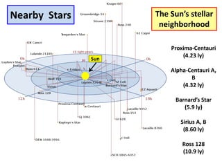
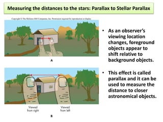
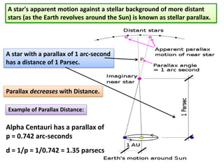
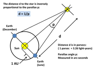
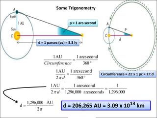
Astonishing Astronomy 101
With Doctor Bones (Don R. Mueller, Ph.D.)
Educator
Entertainer
J
U
G
G
L
E
R
Scientist
Science
Explorer
Chapter 17 – The Stars
Nearby Stars
Proxima-Centauri
(4.23 ly)
Alpha-Centauri A,
B
(4.32 ly)
Barnard’s Star
(5.9 ly)
Sirius A, B
(8.60 ly)
Ross 128
(10.9 ly)
The Sun’s stellar
neighborhood
Sun
Measuring the distances to the stars: Parallax to Stellar Parallax
• As an observer’s
viewing location
changes, foreground
objects appear to
shift relative to
background objects.
• This effect is called
parallax and it can be
used to measure the
distance to closer
astronomical objects.
A star's apparent motion against a stellar background of more distant
stars (as the Earth revolves around the Sun) is known as stellar parallax.
A star with a parallax of 1 arc-second
has a distance of 1 Parsec.
Parallax decreases with Distance.
Example of Parallax Distance:
Alpha Centauri has a parallax of
p = 0.742 arc-seconds
d = 1/p = 1/0.742 = 1.35 parsecs
Earth
(December)
Earth
(June)
Sun
Distance d is in parsecs:
( 1 parsec ≈ 3.26 light-years)
d = 1/p
p
d
1 AU
The distance d to the star is inversely
proportional to the parallax p:
Parallax angle p:
Measured in arc-seconds
Some Trigonometry
d = 1 parsec (pc) = 3.3 ly
Circumference = 2p x 1 pc = 2p d
p = 1 arc-second


360
arcsecond1AU1
nceCircumfere


360
arcsecond1
2
AU1
dp
1,296,000
1
arcseconds1,296,000
arcsecond1
2
AU1

dp
d = 206,265 AU = 3.09 x 10¹³ kmπ2
AU1,296,000
d 
The Effect of Distance on Light
• Light from distant objects
appears to be very dim:
• Why? Because light spreads
out as it travels from source
to destination.
• The further you are from the
source, the dimmer the light.
• The object’s brightness or
amount of light received
from a source, is decreasing.
• The amount of light reaching
us is a star’s brightness.
2
d4
OutputLightTotal
Brightness
p

This is an inverse-square law :
The brightness decreases with the
square of the distance (d) from
the source.
The Inverse-Square Law
Inverse-Square Law
• Stars, like light bulbs, emits light in all
directions: called isotropic radiation.
We see the photons that are heading
in our direction.
• As you move away from the star,
fewer and fewer photons are headed
toward you, thus the star appears to
dim.
• The total amount of energy a star
emits into space is its luminosity
(power) and is measured in Watts.
• Some types of stars have a known
luminosity and we can use the
standard candle to calculate the
distance to the stars.
• The brightness decreases with the
square of the distance from the
star.
• When you move twice as far from
the star, its brightness decreases
by a factor of 22 = 4.
• If we know the total energy
output of a star (luminosity L) and
we can count the number of
photons we receive from the star
(brightness b), we can calculate
its distance d:
b4
L
d
p

The Hipparchus Star Magnitude Scale
• We can quantify the brightness of a
star by assigning it an apparent
magnitude or number in this case:
• Brighter stars have lower numbers.
• Dimmer stars have higher numbers.
• Differences in magnitudes correspond
to ratios in brightness.
• Hipparchus classified the naked-eye
stars into 6 star classes: the brightest
being 1st-class (magnitude) stars and
the faintest being 6th class stars.
• The “brightness” numbers in the star
ranking system of Hipparchus are
called apparent magnitudes.
Absolute Magnitude
• It’s easier to compare the respective luminosities of two
stars if they are at the same distance from the Sun.
• We can calculate how bright the stars would appear if they
were all the same distance from us. Solely as a matter of
convenience we choose 10 parsecs (pc).
• The magnitude of a star “moved” to 10 pc from us is
referred to as its absolute magnitude.
• For example, when a star that is actually closer to 100 pc
from us is placed at the 10 pc standard, its distance d has
decreased by 10 times. In turn, the star’s apparent
brightness would increase by a factor of d2 = 102 =100 (the
inverse square law). The star’s apparent magnitude has
decreased by a factor of 5.
• Years ago, astronomers in their refinement of the star
magnitude scale of Hipparchus, established that a difference
of 5 orders in magnitude corresponded to a factor of 100
times in brightness (intensity).
Relating Magnitude to Brightness Ratio
Magnitude Difference Ratio of Brightness
0 2.5120 = 1:1
0.1 2.5120.1 = 1.10:1
0.5 2.5120.5 = 1.58:1
1 2.5121 = 2.512:1
2 2.5122 = 6.31:1
3 2.5123 = 15.85:1
4 2.5124 = 39.81:1
5 2.5125 = 100:1
10 2.51210 = 104:1
20 2.51220 = 108:1
Photons in Stellar Atmospheres:
Absorption spectra provides, a “fingerprint” for the star’s composition.
The strength of this spectra is determined by the star’s temperature.
Stellar Surface Temperatures
• The peak wavelength emitted by a star shifts with the star’s
surface temperature:
– Hotter stars look blue
– Cooler stars look red
• We can use the star’s color to estimate its surface temperature:
– If a star emits stronger at a particular wavelength  (nm),
then its surface temperature (T) is often given by Wien’s Law:
λ
nmK102.9
T
6


Wien’s Law: Hotter bodies emit more strongly at shorter
wavelengths. When  decreases, T increases.
Measuring the Temperatures of Astronomical Objects
Wien’s Law:
To estimate the temperature T in
degrees Kelvin (K) of stars:
• We just need to measure the
wavelength (max) at which the
star emits the most photons.
• Solving for T:
If the wavelength of maximum emission
(max) for the spectral distribution of the
blackbody curve is plotted versus 1/T, a
straight line is obtained.
maxλ
nmK109.2
T
6


Measuring Temperature T using Wien’s Law
λ
nmK6109.2
T


Measure a star’s brightness
at several wavelengths ()
and then plot the brightness
versus wavelength.
The total emitted radiant energy is
proportional to the 4th power of
the temperature T (K): K4
• If we know an object’s
temperature (T), then we can
calculate how much energy is
being emitted by the object,
using the Stefan-Boltzmann law:
• The power P is in Watts, area A
is in square meters and the
Stefan-Boltzmann constant:
 = 5.6710-8 Watts/m2K4
4
σT
A
P

Stefan-Boltzmann Law
Luminosity increases rapidly with temperature
The Stefan-Boltzmann Law
A star’s luminosity is related to both a star’s size and temperature:
(a) Hotter stars emit more. (b) Larger stars emit more.
Each square meter
of the star’s surface
emits T4 watts.
The total energy radiated per
second is the Luminosity L:
A spherical star of radius R, has a surface area S = 4pR2
42
σTRπ4L 
Spectral Classification
• Spectral classification
system: By temperature
Hotter stars are O type
Cooler stars are M type
• New Types: L and T
– Cooler than M
• From hottest to coldest, they are:
O-B-A-F-G-K-M
– Mnemonics: “Oh, Be A Fine
Girl/Guy, Kiss Me
– Or: Only Bad Astronomers Forget
Generally Known Mnemonics
Spectral Classification
• Application of Wien’s law and theoretical calculations show
that temperatures range from more than 30,000 K for O stars
to less than 3500 K for M stars.
• Because a star’s spectral type is set by its temperature, its
type also indicates its color; ranging from violet-blue colors
for O and B stars, to reddish colors for K and M stars.
• To distinguish still smaller gradations in temperature,
astronomers subdivide each type by adding a numerical
suffix—for example, B0, B1, B2,..., B9—with the smaller
numbers indicating progressively higher temperatures.
Summary of Spectral Types
Spectral Type Temperature Range (K) Features
O Hotter than 30,000 Ionized helium, weak hydrogen.
B 10,000-30,000 Neutral helium, hydrogen stronger.
A 7500-10,000 Hydrogen very strong.
F 6000-7500 Hydrogen weaker, metals—especially
ionized Ca—moderate.
G 5000-6000 Ionized Ca strong, hydrogen weak.
K 3500-5000 Metals strong, CH and CN molecules
appearing.
M 2000-3500 Molecules strong: especially TiO and
water.
L 1300-2000 TiO disappears. Strong lines of metal
hydrides, water and reactive metals
such as potassium and cesium.
T 900?-1300? Strong lines of water and methane.
23
O-B-A-F-G-K-M SchemeStellar Spectral Classes
A convenient tool for organizing stars
• A star’s luminosity depends on its temperature and diameter.
A Hertzsprung-Russell diagram is used to find trends in this relationship.
Constructing
Hertzsprung-Russell
(H-R) Diagrams
The H-R Diagram• A star’s location on the H-R
diagram is given by:
temperature (x-axis) and
luminosity (y-axis).
• Many stars are located on a
diagonal line running from
cool, dim stars to hot bright
stars: The Main Sequence
• Other stars are cooler and
more luminous than main
sequence stars:
Have large diameters
(Red and Blue) Giant stars
• Some stars are hotter, yet
less luminous than main
sequence stars:
Have small diameters
White Dwarf stars
H-R Diagram
• Most stars are
found on the
main sequence.
• Giants
• Supergiants
• White dwarfs
Main Sequence
White Dwarfs
Giants
Super Giants
Temperature (K)
Luminosity Spectral Type
27
Lines of constant Radius in the H-R diagram
 Main sequence
• B stars: R ~ 10 RSun
• M stars: R ~ 0.1 RSun
 Betelgeuse:
R ~ 1,000 Rsun
(Larger than 1 AU)
 White dwarfs:
R ~ 0.01 Rsun
(A few Earth radii)
l
A Family of Stars
Stars of all sizes
The Mass-Luminosity Relation• When we look for trends in
stellar masses, we notice
something interesting:
Low mass main sequence stars
tend to be cooler and dimmer.
High mass main sequence stars
tend to be hotter and brighter.
• Mass-Luminosity Relation:
Massive stars burn brighter.
5.3
ML 
31
Mass-Luminosity Plot
L = M3.5
Stellar Luminosity Classes
Class Description Example
Ia Bright
supergiants
Betelgeuse, Rigel (brightest stars in Orion)
Ib Supergiants Antares (brightest star in Scorpius)
II Bright giants Polaris (the North Star)
III Ordinary giants Arcturus (brightest star in northern
constellation Boötes)
IV Subgiants Procyon A (brightest star in Canis Minor)
V Main sequence The Sun, Sirius A (brightest star in sky, in
Canis Majoris)
Luminosity Classes
Ia Bright supergiant
Ib Supergiant
II Bright giant
III Giant
IV Subgiant
V Main sequence
Sun: G2 V
Rigel: B8 Ia
Betelgeuse: M2 Iab
Measuring Star Diameters
by employing
Interferometric Techniques
• Stars are simply too far away to easily
measure their diameters.
• Atmospheric blurring and telescope
effects smear out the light.
• Interestingly, we can combine the light
from multiple telescopes in a process
called astronomical interferometry:
Two telescopes separated by a distance of
300 meters have nearly the same
resolution as a single telescope with a
diameter of 300 meters.
The diameter of the red giant Betelgeuse
was determined using this technique.
Speckle interferometry, which
employs Fourier analysis, uses
multiple images from the same
telescope to increase resolution.
Using eclipsing binary systems to measure stellar diameters
Types of Binary Stars• Stars found orbiting other stars
are called binary stars.
Three types are known:
1. Visual Binary - If we can see from
photos taken over time that the stars
are orbiting each other, the system is
a visual binary.
2. Spectroscopic Binary - If the stars
are so close together that their
spectra blur together, the system is
called a spectroscopic binary.
3. Eclipsing Binary - If the stars are
oriented edge-on to the Sun, one
star will periodically eclipse the
other star in the system. These are
known as eclipsing binaries.
Using the Doppler Shift to detect binary systems
• As a star in a binary system moves away from us, its spectrum is
shifted towards red wavelengths. As it moves toward us again, the
spectrum is shifted toward blue wavelengths.
• This Doppler Shifting allows us to detect some binaries.
Measuring Stellar Masses with Binary Stars
This technique gives us the combined mass of the two stars.
The Center of Mass COM: (1) calculate the combined mass,
(2) using the distance from the center of mass COM, we can
calculate each star’s mass.
• In a binary system, the two
stars orbit a common COM.
• The masses and distances
from the COM are related
through:
MA × aA = MB × aB
• If the stars are of equal
mass, the COM is directly
between them.
• If the stars are of unequal
mass, the COM is closer to
the more massive star.

Astonishing Astronomy 101 - Chapter 17

  • 1.
    Astonishing Astronomy 101 WithDoctor Bones (Don R. Mueller, Ph.D.) Educator Entertainer J U G G L E R Scientist Science Explorer
  • 2.
    Chapter 17 –The Stars
  • 3.
    Nearby Stars Proxima-Centauri (4.23 ly) Alpha-CentauriA, B (4.32 ly) Barnard’s Star (5.9 ly) Sirius A, B (8.60 ly) Ross 128 (10.9 ly) The Sun’s stellar neighborhood Sun
  • 4.
    Measuring the distancesto the stars: Parallax to Stellar Parallax • As an observer’s viewing location changes, foreground objects appear to shift relative to background objects. • This effect is called parallax and it can be used to measure the distance to closer astronomical objects.
  • 5.
    A star's apparentmotion against a stellar background of more distant stars (as the Earth revolves around the Sun) is known as stellar parallax. A star with a parallax of 1 arc-second has a distance of 1 Parsec. Parallax decreases with Distance. Example of Parallax Distance: Alpha Centauri has a parallax of p = 0.742 arc-seconds d = 1/p = 1/0.742 = 1.35 parsecs
  • 6.
    Earth (December) Earth (June) Sun Distance d isin parsecs: ( 1 parsec ≈ 3.26 light-years) d = 1/p p d 1 AU The distance d to the star is inversely proportional to the parallax p: Parallax angle p: Measured in arc-seconds
  • 7.
    Some Trigonometry d =1 parsec (pc) = 3.3 ly Circumference = 2p x 1 pc = 2p d p = 1 arc-second   360 arcsecond1AU1 nceCircumfere   360 arcsecond1 2 AU1 dp 1,296,000 1 arcseconds1,296,000 arcsecond1 2 AU1  dp d = 206,265 AU = 3.09 x 10¹³ kmπ2 AU1,296,000 d 
  • 8.
    The Effect ofDistance on Light • Light from distant objects appears to be very dim: • Why? Because light spreads out as it travels from source to destination. • The further you are from the source, the dimmer the light. • The object’s brightness or amount of light received from a source, is decreasing. • The amount of light reaching us is a star’s brightness. 2 d4 OutputLightTotal Brightness p  This is an inverse-square law : The brightness decreases with the square of the distance (d) from the source.
  • 9.
  • 10.
    Inverse-Square Law • Stars,like light bulbs, emits light in all directions: called isotropic radiation. We see the photons that are heading in our direction. • As you move away from the star, fewer and fewer photons are headed toward you, thus the star appears to dim. • The total amount of energy a star emits into space is its luminosity (power) and is measured in Watts. • Some types of stars have a known luminosity and we can use the standard candle to calculate the distance to the stars. • The brightness decreases with the square of the distance from the star. • When you move twice as far from the star, its brightness decreases by a factor of 22 = 4. • If we know the total energy output of a star (luminosity L) and we can count the number of photons we receive from the star (brightness b), we can calculate its distance d: b4 L d p 
  • 11.
    The Hipparchus StarMagnitude Scale • We can quantify the brightness of a star by assigning it an apparent magnitude or number in this case: • Brighter stars have lower numbers. • Dimmer stars have higher numbers. • Differences in magnitudes correspond to ratios in brightness. • Hipparchus classified the naked-eye stars into 6 star classes: the brightest being 1st-class (magnitude) stars and the faintest being 6th class stars. • The “brightness” numbers in the star ranking system of Hipparchus are called apparent magnitudes.
  • 12.
    Absolute Magnitude • It’seasier to compare the respective luminosities of two stars if they are at the same distance from the Sun. • We can calculate how bright the stars would appear if they were all the same distance from us. Solely as a matter of convenience we choose 10 parsecs (pc). • The magnitude of a star “moved” to 10 pc from us is referred to as its absolute magnitude. • For example, when a star that is actually closer to 100 pc from us is placed at the 10 pc standard, its distance d has decreased by 10 times. In turn, the star’s apparent brightness would increase by a factor of d2 = 102 =100 (the inverse square law). The star’s apparent magnitude has decreased by a factor of 5. • Years ago, astronomers in their refinement of the star magnitude scale of Hipparchus, established that a difference of 5 orders in magnitude corresponded to a factor of 100 times in brightness (intensity).
  • 13.
    Relating Magnitude toBrightness Ratio Magnitude Difference Ratio of Brightness 0 2.5120 = 1:1 0.1 2.5120.1 = 1.10:1 0.5 2.5120.5 = 1.58:1 1 2.5121 = 2.512:1 2 2.5122 = 6.31:1 3 2.5123 = 15.85:1 4 2.5124 = 39.81:1 5 2.5125 = 100:1 10 2.51210 = 104:1 20 2.51220 = 108:1
  • 14.
    Photons in StellarAtmospheres: Absorption spectra provides, a “fingerprint” for the star’s composition. The strength of this spectra is determined by the star’s temperature.
  • 15.
    Stellar Surface Temperatures •The peak wavelength emitted by a star shifts with the star’s surface temperature: – Hotter stars look blue – Cooler stars look red • We can use the star’s color to estimate its surface temperature: – If a star emits stronger at a particular wavelength  (nm), then its surface temperature (T) is often given by Wien’s Law: λ nmK102.9 T 6   Wien’s Law: Hotter bodies emit more strongly at shorter wavelengths. When  decreases, T increases.
  • 16.
    Measuring the Temperaturesof Astronomical Objects Wien’s Law: To estimate the temperature T in degrees Kelvin (K) of stars: • We just need to measure the wavelength (max) at which the star emits the most photons. • Solving for T: If the wavelength of maximum emission (max) for the spectral distribution of the blackbody curve is plotted versus 1/T, a straight line is obtained. maxλ nmK109.2 T 6  
  • 17.
    Measuring Temperature Tusing Wien’s Law λ nmK6109.2 T   Measure a star’s brightness at several wavelengths () and then plot the brightness versus wavelength.
  • 18.
    The total emittedradiant energy is proportional to the 4th power of the temperature T (K): K4 • If we know an object’s temperature (T), then we can calculate how much energy is being emitted by the object, using the Stefan-Boltzmann law: • The power P is in Watts, area A is in square meters and the Stefan-Boltzmann constant:  = 5.6710-8 Watts/m2K4 4 σT A P  Stefan-Boltzmann Law Luminosity increases rapidly with temperature
  • 19.
    The Stefan-Boltzmann Law Astar’s luminosity is related to both a star’s size and temperature: (a) Hotter stars emit more. (b) Larger stars emit more. Each square meter of the star’s surface emits T4 watts. The total energy radiated per second is the Luminosity L: A spherical star of radius R, has a surface area S = 4pR2 42 σTRπ4L 
  • 20.
    Spectral Classification • Spectralclassification system: By temperature Hotter stars are O type Cooler stars are M type • New Types: L and T – Cooler than M • From hottest to coldest, they are: O-B-A-F-G-K-M – Mnemonics: “Oh, Be A Fine Girl/Guy, Kiss Me – Or: Only Bad Astronomers Forget Generally Known Mnemonics
  • 21.
    Spectral Classification • Applicationof Wien’s law and theoretical calculations show that temperatures range from more than 30,000 K for O stars to less than 3500 K for M stars. • Because a star’s spectral type is set by its temperature, its type also indicates its color; ranging from violet-blue colors for O and B stars, to reddish colors for K and M stars. • To distinguish still smaller gradations in temperature, astronomers subdivide each type by adding a numerical suffix—for example, B0, B1, B2,..., B9—with the smaller numbers indicating progressively higher temperatures.
  • 22.
    Summary of SpectralTypes Spectral Type Temperature Range (K) Features O Hotter than 30,000 Ionized helium, weak hydrogen. B 10,000-30,000 Neutral helium, hydrogen stronger. A 7500-10,000 Hydrogen very strong. F 6000-7500 Hydrogen weaker, metals—especially ionized Ca—moderate. G 5000-6000 Ionized Ca strong, hydrogen weak. K 3500-5000 Metals strong, CH and CN molecules appearing. M 2000-3500 Molecules strong: especially TiO and water. L 1300-2000 TiO disappears. Strong lines of metal hydrides, water and reactive metals such as potassium and cesium. T 900?-1300? Strong lines of water and methane.
  • 23.
  • 24.
    A convenient toolfor organizing stars • A star’s luminosity depends on its temperature and diameter. A Hertzsprung-Russell diagram is used to find trends in this relationship. Constructing Hertzsprung-Russell (H-R) Diagrams
  • 25.
    The H-R Diagram•A star’s location on the H-R diagram is given by: temperature (x-axis) and luminosity (y-axis). • Many stars are located on a diagonal line running from cool, dim stars to hot bright stars: The Main Sequence • Other stars are cooler and more luminous than main sequence stars: Have large diameters (Red and Blue) Giant stars • Some stars are hotter, yet less luminous than main sequence stars: Have small diameters White Dwarf stars
  • 26.
    H-R Diagram • Moststars are found on the main sequence. • Giants • Supergiants • White dwarfs Main Sequence White Dwarfs Giants Super Giants Temperature (K) Luminosity Spectral Type
  • 27.
    27 Lines of constantRadius in the H-R diagram  Main sequence • B stars: R ~ 10 RSun • M stars: R ~ 0.1 RSun  Betelgeuse: R ~ 1,000 Rsun (Larger than 1 AU)  White dwarfs: R ~ 0.01 Rsun (A few Earth radii) l
  • 28.
  • 29.
  • 30.
    The Mass-Luminosity Relation•When we look for trends in stellar masses, we notice something interesting: Low mass main sequence stars tend to be cooler and dimmer. High mass main sequence stars tend to be hotter and brighter. • Mass-Luminosity Relation: Massive stars burn brighter. 5.3 ML 
  • 31.
  • 32.
    Stellar Luminosity Classes ClassDescription Example Ia Bright supergiants Betelgeuse, Rigel (brightest stars in Orion) Ib Supergiants Antares (brightest star in Scorpius) II Bright giants Polaris (the North Star) III Ordinary giants Arcturus (brightest star in northern constellation Boötes) IV Subgiants Procyon A (brightest star in Canis Minor) V Main sequence The Sun, Sirius A (brightest star in sky, in Canis Majoris)
  • 33.
    Luminosity Classes Ia Brightsupergiant Ib Supergiant II Bright giant III Giant IV Subgiant V Main sequence Sun: G2 V Rigel: B8 Ia Betelgeuse: M2 Iab
  • 34.
    Measuring Star Diameters byemploying Interferometric Techniques • Stars are simply too far away to easily measure their diameters. • Atmospheric blurring and telescope effects smear out the light. • Interestingly, we can combine the light from multiple telescopes in a process called astronomical interferometry: Two telescopes separated by a distance of 300 meters have nearly the same resolution as a single telescope with a diameter of 300 meters. The diameter of the red giant Betelgeuse was determined using this technique. Speckle interferometry, which employs Fourier analysis, uses multiple images from the same telescope to increase resolution.
  • 35.
    Using eclipsing binarysystems to measure stellar diameters
  • 36.
    Types of BinaryStars• Stars found orbiting other stars are called binary stars. Three types are known: 1. Visual Binary - If we can see from photos taken over time that the stars are orbiting each other, the system is a visual binary. 2. Spectroscopic Binary - If the stars are so close together that their spectra blur together, the system is called a spectroscopic binary. 3. Eclipsing Binary - If the stars are oriented edge-on to the Sun, one star will periodically eclipse the other star in the system. These are known as eclipsing binaries.
  • 37.
    Using the DopplerShift to detect binary systems • As a star in a binary system moves away from us, its spectrum is shifted towards red wavelengths. As it moves toward us again, the spectrum is shifted toward blue wavelengths. • This Doppler Shifting allows us to detect some binaries.
  • 38.
    Measuring Stellar Masseswith Binary Stars This technique gives us the combined mass of the two stars.
  • 39.
    The Center ofMass COM: (1) calculate the combined mass, (2) using the distance from the center of mass COM, we can calculate each star’s mass. • In a binary system, the two stars orbit a common COM. • The masses and distances from the COM are related through: MA × aA = MB × aB • If the stars are of equal mass, the COM is directly between them. • If the stars are of unequal mass, the COM is closer to the more massive star.