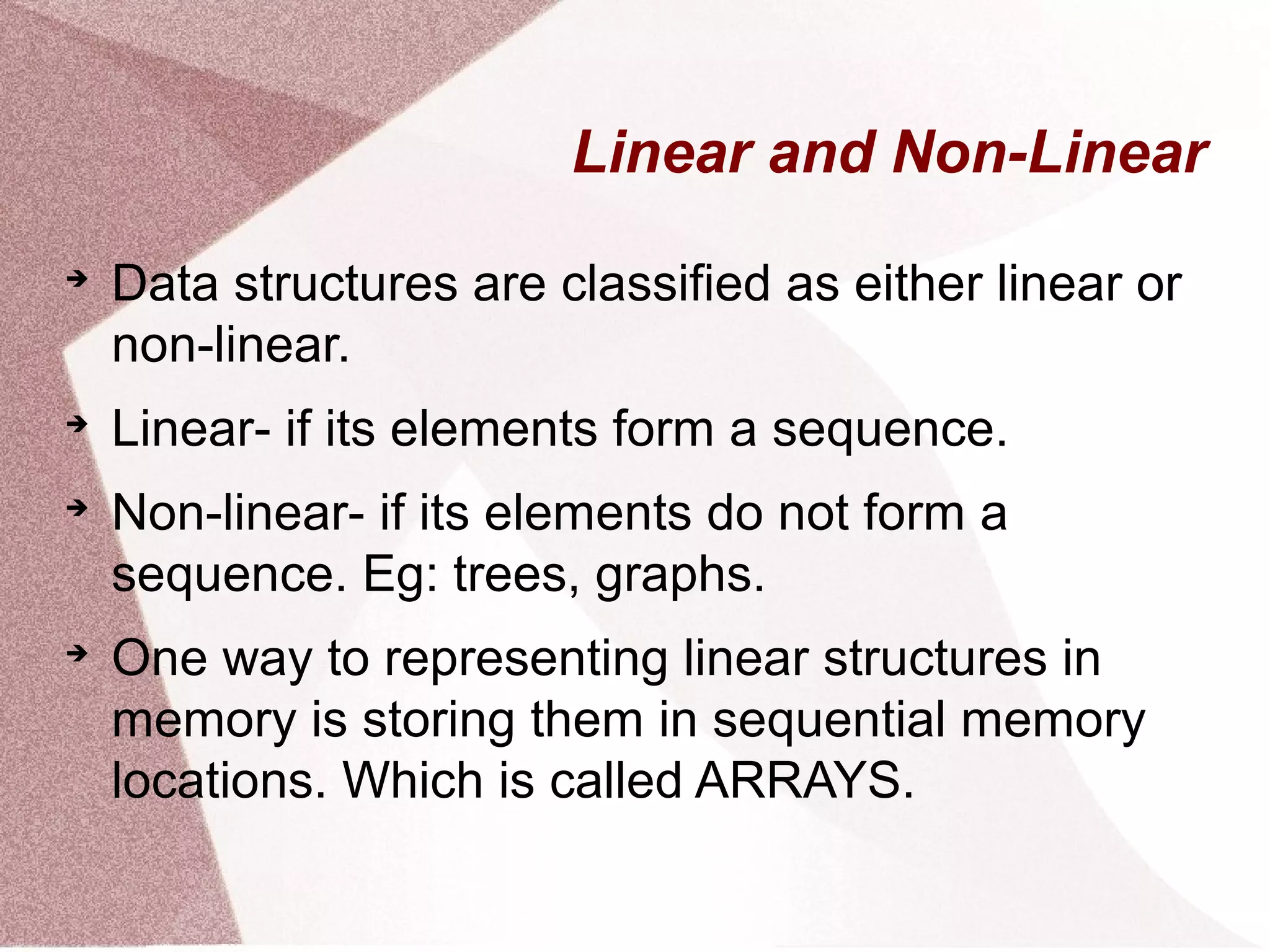
The document discusses different data structures and their properties. It explains that data structures can be linear or non-linear. Linear data structures like arrays have elements arranged in a sequence, while non-linear structures like trees and graphs do not. It then focuses on linear data structures and their representation in memory using arrays and linked lists. Key operations on linear structures like traversal, search, insertion and deletion are also summarized.

1. Linear and Non-Linear

Data structures are classified as either linear or
non-linear.

Linear- if its elements form a sequence.

Non-linear- if its elements do not form a
sequence. Eg: trees, graphs.

One way to representing linear structures in
memory is storing them in sequential memory
locations. Which is called ARRAYS.

2. Other way is to have a linera relationship between
the elements represented by means of pointer
or links.
This is called LINKED LISTS.

3. INSERTING

Consider an array DATA. We want to
insert an element at Kth position in
DATA.

First we will have to move down all the
elements starting from K, one by one.

We start moving, starting from the
bottom.

4. OPERATIONS PERFORMED

Operations performed on a linear structure are:

Traversal.

Search

Insertion

Deletion

Sorting

Merging.

5. CRITERIA FOR CHOOSING DATA
STRUCTURES
The criteria of choosing a given data structure
depends on the frequency with which one
performs these operations.

6. ARRAYS

Easy to traverse, search and sort.

So used for permanent storage of data, that is
not changed often.

A LINEAR ARRAY is a list of a finite number n of
homogeneous data elements such that:

The elements of the array are referenced by an
index set consisting of consecutive numbers.

The elements of the array are stored in
consecutive memory locations.

7. The number n is called length or size of array.
If not otherwise stated we will assume that the
index set consists of integers 1,2,3,4....n.
The length of array can be obtained by formula:
Length= UB-LB +1
Where UB is the largest index.
And LB is the smallest index.

8. 
Each programming language has its own way of
declaring the arrays.

But all languages must provide following 3
things:

Name of the array.

Data type

Index set.

9. REPRESENTATIONS IN MEMORY

As discussed earlier.

Computer does not keep track of each memory
location.

It only keeps track of the first memory location
of the array called BASE(LA).

Other memory locations are calculated by
formula:

LOC(LA[K])= base (LA) + w(k-lowerbound)

w=number of words per memory cell of array.

10. 
Things to note:

The time taken to find each memory location is
same.

Means time taken to find any location in an
array is independent of the length of the array.

Any memory location can be located without
traversing other memory locations.

11. TRAVERSING

Traversing means visiting each element of the
array exactly once.

Eg: if i want to print all the elements of the array.

Or if i want to count the number of elements of
an array, or if i want to print the elements of
array with certain property.

We can name any of this work as PROCESS

12. ALGORITHM OF TRAVERSING.

13. INSERTING AND
DELETING IN AN ARRAY

Let A be an array.

INSERTING refers to the operation of
adding another element in array.

DELETING refers to the operation of
removing one element from array.

Inserting at end is easy, given an extra
memory space at the end.

If inserting at the middle of the array,
then on an average we need to move
half of the elements downwards.

14. 
Similarly deleting from the end is quite
easy.

But if deleting from middle of array, on
average we will have to move half of the
elements of the array upwards.

Show by drawing a diagram

15. 
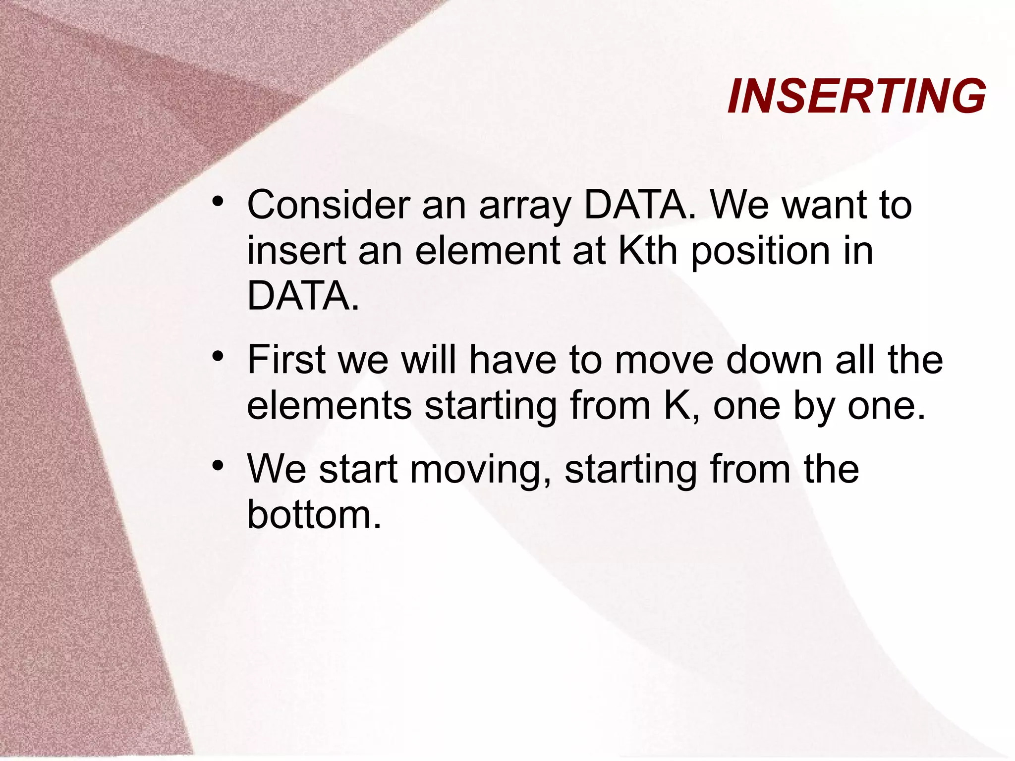
Let LA be a linear array with N
elements. We want to insert an element
at Kth position.
1. Set J:=N.
2. Repeat steps 3 and 4 till J >=K
3. Set LA[J+1]:= LA[J]
4. Set J:=J-1
5. Set LA[K]:= ITEM.
6. Set N:=N+1

16. DELETING

After deleting an element from Kth
position we will have to move each
element one position UP.

Let LA be a linear array with N number
of elements
1. Set ITEM:= LA[K].
2. Repeart for J=K to N-1.
3.Set LA[J] := LA[J+1].
4.Set N:= N-1

17. BUBBLE SORT

Sorting means rearranging the elements
of array so that they are is
increasing/decreasing order.

Show an eg of sorting.

The concept behind bubble sort is that
suppose A is the array. First we
compare A[1] and A[2]. If A[1] is greater
than A[2] then we interchange the
positions of both, else not.

18. 
Then we check A[2] and A[3]. If A[2] is
greater than A[3] then we interchange
their positions, else not.

So on till A[n]. this whole series of
comparison is called ONE PASS.

After completion of Pass 1, the largest
element will be at the end.

Means in Pass 1, N-1 comparisons
have been made.

19. 
At the end of pass 1, the largest
element in the list is at its place.

Then we repeat same process for Pass
2. but now the number of comparisons
is N-2.

And so on.

In each pass the number of
comparisons will be decreasing.

We will have total N-1 passes.

20. 
Here DATA us ab array with N elements.
1) Repeat steps 2 and 3 for K=1 to N-1.
(for keeping track of number of pass)
2) Set PTR:=1.
3) Repeat while PTR <= N-K(for
number of comparisons)
1) If DATA[PTR] > DATA[PTR-1], then
Interchange DATA[PTR] and
DATA[PTR+1].
1) Set PTR:=PTR+1
4) EXIT.

21. SEARCHING.

Searching refers to the operation of
finding the location LOC of ITEM in array
DATA, or printing some message that
ITEM does not appear in array.

Successful search: if ITEM is found.

Many different searching algorithms.

Criteria for choosing certain algo is the
way in which info is organized in DATA.

22. 
The complexity of searching algo is
measured in terms of number f(n) of
comparison required to find ITEM in
DATA, where DATA contains “n”
elements.

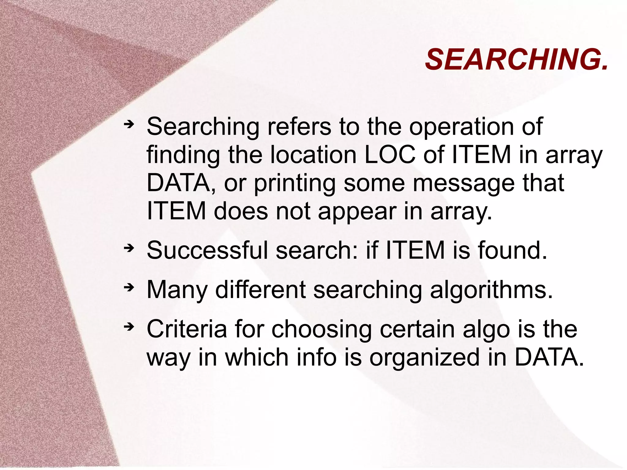
23. LINEAR SEARCH

Suppose DATA is a linear array with n
elements.

We want to search ITEM in DATA.

First we test whether DATA[1]=ITEM,
then we check whether DATA[2]=ITEM
and so on.

This method which traverses DATA
sequentially to loacate item is called
“linear search” or “sequential search”.

24. 
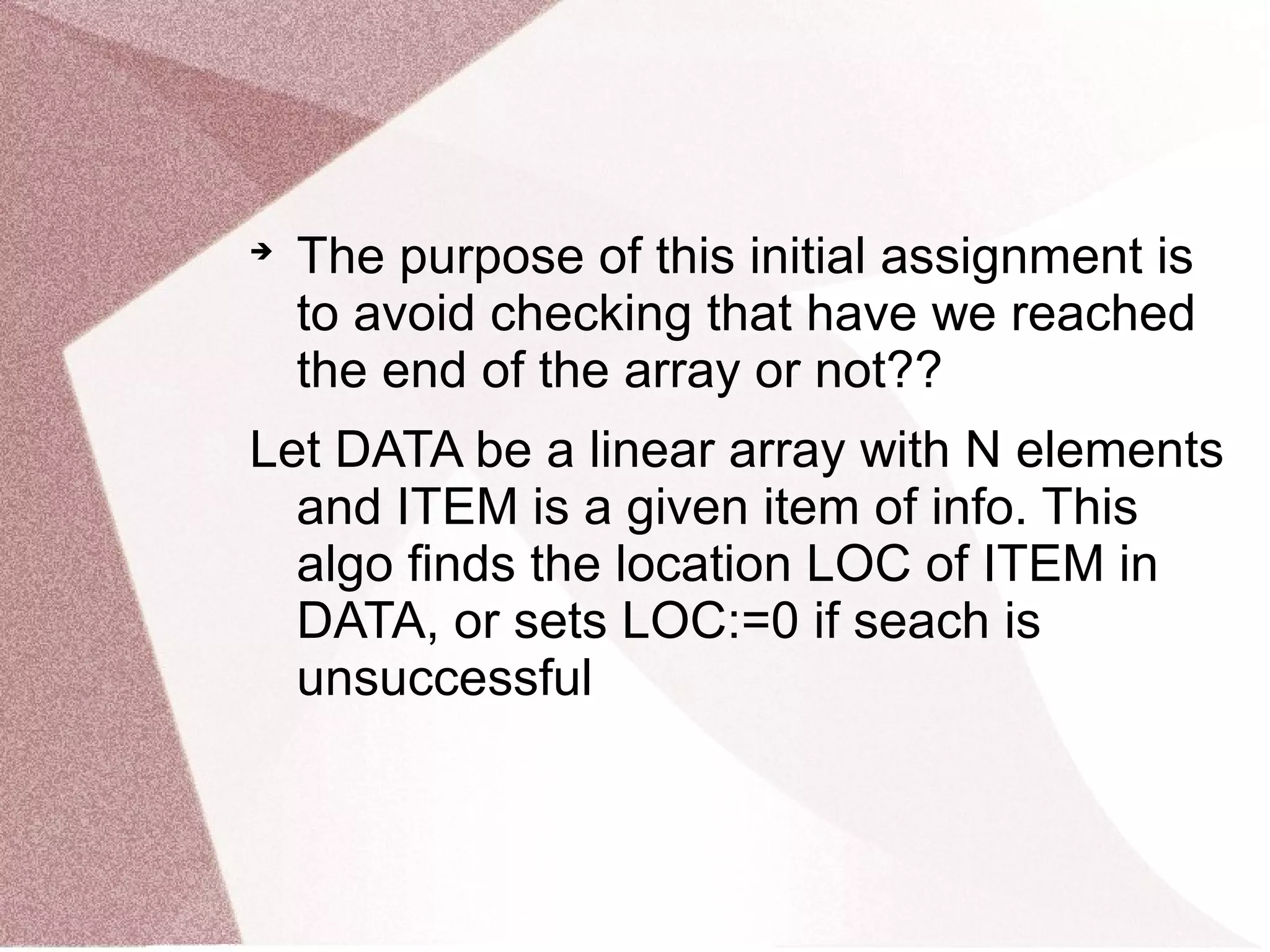
We first insert ITEM to be searched at
DATA[n+1] location, ie, at the last
position of the array.

LOC denotes the location where ITEM
first occurs in DATA.

Means if at the end of algo we get LOC=
n+1, it means the search was
unsuccessful, cause WE have inserted
ITEM at n+1.

25. 
The purpose of this initial assignment is
to avoid checking that have we reached
the end of the array or not??
Let DATA be a linear array with N elements
and ITEM is a given item of info. This
algo finds the location LOC of ITEM in
DATA, or sets LOC:=0 if seach is
unsuccessful

26. ALGO
1.Set DATA[N+1]= item.(insert at end)
2.Set LOC:=1
3.Repeat while DATA[LOC]!= ITEM.(search)
Set LOC:= LOC +1.
1.If LOC= N+1, Then set LOC:=0.
2.Exit.

27. COMPLEXITY OF LINEAR
SEARCH

Complexity is measured y the number
f(n) of comparisons required to find
ITEM in DATA where DATA contains “n”
elements.

We discuss about AVERAGE CASE and
WORST CASE.

Worst case is if the item doesnot occur
in the array. So in this case algo
requires:

f(n)= n+1 comparisons.

Thus runnign time is proportional to n.

28. For average case f(n)= (n+1)/2.

29. BINARY SEARCH

Suppose data in array is sorted in
increasing numerical order.

There is an extremely efficient algo for
this called BINARY SEARCH.

Example of telephone directory.

Suppose following is the array DATA:
DATA[BEG], DATA[BEG+1], DATA[BEG+2],.....,
DATA[END].

Means we have to define a BEG and an END.

30. 
During each stage our search is reduced
to a segment of DATA.

The algo compares ITEM with the
middle element DATA[MID] of the
segment, where MID =
int((BEG+END)/2).

INT used because we want an integer
value of MID.

If DATA[MID]= ITEM, then search is
successful, and LOC:=MID.

31. 
Otherwise search is narrowed down to a
new segment, which is obtained as:
1. If ITEM< DATA[MID], then ITEM
appears in the left half, so reset END
as:

END= MID-1, and begin search again.
1. If ITEM> DATA[MID], then ITEM
appears in the right half, so reset BEG
as:

BEG= MID+1, and begin search
again.

First we begin with BEG=LB n END=UB.

32. 
If the ITEM is found, then it will be found
at the MID.

Let DATA is a sorted array, with lower
bound LB, upper bound UP. ITEM is a
given item of information. The variables
BEG, END and MID are used. Algo finds
location LOC of ITEM in DATA or sets
LOC = NULL.

33. 1. Set BEG=LB, END=UB,
MID=int((BEG+END)/2).
2.Repeat steps 3 and 4 while BEG<=END and
DATA[MID]!=ITEM.
3. If ITEM < DATA[MID], then:

Set END:= MID - 1.

Else

Set BEG= MID + 1.
1. Set MID = int((BEG+END)/2).

34. 1. If DATA[MID] = ITEM, then

Set LOC=MID
Else

Set LOC=NULL.
1.END

When item doesnot appear in DATA, the
algorithm eventually arrives at a position
where BEG=END=MID.

35. Complexity and
Disadvantages

Complexity is:

f(n)=log 2 n + 1

Limitations of this algo:

Requires array to be sorted.

Which is quite expensive when new
elements are inserted and deleted
frequently.

36. RECORDS AND RECORD
STRUCTURE

A “record” is a collection of related data
items.

Each data item is called “attribute”.

Record is a collection of data items, but
it differs from linear array.

Array is collection of homogeneous data,
whereas record is a collection of
“nonhomogeneous” data.

We can see a record as “structure” in C.

37. Memory
representation:Parallel
Array

Record cannot be stored in linear array,
cause of its nonhomogeneousity.

So languages have build in “record
structures”, like structures in C.

Consider a record of Newbord baby
which consists of following:

38. 
name(string)

gender(char)

Birthday

Month

Day

Year

Father

Name

age
Mother
 Name
 age

39. 
Now data in each array having same
subscript belongs to same record.

These arrays used to store various
attributes of array are called PARALLEL
ARRAYS.

40. – Name
– Gender
– Month
– Day
– Year
– Father name
– Father age
– Mother name
– Mother age.

41. 
Such a record can be saved in a
structure.

Discuss about structures.

Suppose a programming language doest
not have anything like structure to
represent such kind of record.

In such case we ll have to make 9 arrays
as:

42. MATRICES AND VECTORS
Anything stored in linear array can be said
as Vector.
Anything stored in 2 dimenssional array
can be said as Matrix.
Show some examples of vector and matrix
arithematic.

43. SPARCE MATRIX.

Matrix with relatively high proportion of
zero entries are called sparse matrices.
4
3 -5
6 3 2
4 2 12 1
4 5 6 56 3
5 2
2 6
6 7
8 9
TRIANGULAR
MATRIX
TRIDIAGONAL
MATRIX