Approximation in Value Space using Aggregation, with Applications to POMDPs and Cybersecurity
1.
Topics in ReinforcementLearning:
AlphaZero, ChatGPT, Neuro-Dynamic Programming,
Model Predictive Control, Discrete Optimization, Applications
Arizona State University
Course CSE 691, Spring 2025
Links to Class Notes, Videolectures, and Slides at
http://web.mit.edu/dimitrib/www/RLbook.html1
Dr. Kim Hammar (khammar1@asu.edu), Prof. Dimitri P. Bertsekas
(dimitrib@mit.edu), and Dr. Yuchao Li (yuchaoli@asu.edu)
Guest Lecture
Approximation in Value Space using Aggregation,
with Applications to POMDPs and Cybersecurity
1
Dimitri P. Bertsekas. A Course in Reinforcement Learning. 2nd edition. Athena Scientific, 2025.
Kim Hammar Approximation by Aggregation 2 April, 2025 1 / 39
2.
Aggregation is AForm of Problem Simplification
Original problem Simplified problem Simplified solution
x1 x2 . . .
y1 y2 . . .
z1 z2 . . .
x y
z
x y
z
u = 1
u = 0
u = 2
Aggregation
The Aggregation Methodology
1 Combine groups of similar states into aggregate states.
2 Formulate an aggregate dynamic programming problem based on these states.
3 Solve the aggregate problem using some computational method.
4 Use the solution to the aggregate problem to compute a cost function approximation
for the original problem.
Kim Hammar Approximation by Aggregation 2 April, 2025 2 / 39
3.
Aggregation is AForm of Problem Simplification
Original problem Simplified problem Simplified solution
x1 x2 . . .
y1 y2 . . .
z1 z2 . . .
x y
z
x y
z
u = 1
u = 0
u = 2
Aggregation
The Aggregation Methodology
1 Combine groups of similar states into aggregate states.
2 Formulate an aggregate dynamic programming problem based on these states.
3 Solve the aggregate problem using some computational method.
4 Use the solution to the aggregate problem to compute a cost function approximation
for the original problem.
Kim Hammar Approximation by Aggregation 2 April, 2025 2 / 39
4.
Aggregation is AForm of Problem Simplification
Original problem Simplified problem Simplified solution
x1 x2 . . .
y1 y2 . . .
z1 z2 . . .
x y
z
x y
z
u = 1
u = 0
u = 2
Aggregation
The Aggregation Methodology
1 Combine groups of similar states into aggregate states.
2 Formulate an aggregate dynamic programming problem based on these states.
3 Solve the aggregate problem using some computational method.
4 Use the solution to the aggregate problem to compute a cost function approximation
for the original problem.
Kim Hammar Approximation by Aggregation 2 April, 2025 2 / 39
5.
Aggregation is AForm of Problem Simplification
Original problem Simplified problem Simplified solution
x1 x2 . . .
y1 y2 . . .
z1 z2 . . .
x y
z
x y
z
u = 1
u = 0
u = 2
Aggregation
The Aggregation Methodology
1 Combine groups of similar states into aggregate states.
2 Formulate an aggregate dynamic programming problem based on these states.
3 Solve the aggregate problem using some computational method.
4 Use the solution to the aggregate problem to compute a cost function approximation
for the original problem.
Kim Hammar Approximation by Aggregation 2 April, 2025 2 / 39
6.
Outline
1 Aggregation withRepresentative States
2 Example: Aggregation with Representative States for POMDPs
3 General Aggregation Methodology
4 Case study: Aggregation for Cybersecurity
Kim Hammar Approximation by Aggregation 2 April, 2025 3 / 39
7.
Outline
1 Aggregation withRepresentative States
2 Example: Aggregation with Representative States for POMDPs
3 General Aggregation Methodology
4 Case study: Aggregation for Cybersecurity
Kim Hammar Approximation by Aggregation 2 April, 2025 3 / 39
8.
Outline
1 Aggregation withRepresentative States
2 Example: Aggregation with Representative States for POMDPs
3 General Aggregation Methodology
4 Case study: Aggregation for Cybersecurity
Kim Hammar Approximation by Aggregation 2 April, 2025 3 / 39
9.
Outline
1 Aggregation withRepresentative States
2 Example: Aggregation with Representative States for POMDPs
3 General Aggregation Methodology
4 Case study: Aggregation for Cybersecurity
Kim Hammar Approximation by Aggregation 2 April, 2025 3 / 39
10.
Reminder on Notation
Statespace: X = {1, . . . , n}, states are denoted by i, j.
Control constraint set: U(i).
Cost of transitioning from state i to j given control u: g(i, u, j).
Cost-to-go from state i: J(i).
Discount factor: α.
Probability of transitioning from state i to j given control u: pij (u).
▶ Equivalent formulation: xk+1 = f (xk , uk , wk ).
i j
pij (u), g(i, u, j)
Kim Hammar Approximation by Aggregation 2 April, 2025 4 / 39
11.
Representative States
Introduce asubset A of the original states 1, . . . , n, called representative states.
We use i, j to denote original states and x, y to denote representative states. mi
u∈U
π/4 Sample State xs
k Sample Contr
Representative States Critic A
Sample Q-Factor βs
k = gs
k + ˜
Jk+1(x
Policy Q-Factor Evaluation Ev
min
u∈U(i)
n
!
j=1
pij(u)
"
g(i, u, j) +
π/4 Sample State xs
k Sample Control us
k Sample Next Sta
Representative States (Coarse Grid) Critic Actor
Range of Weighted Projections States (Fine Grid)
Sample Q-Factor βs
k = gs
k + ˜
Jk+1(xs
k+1) ˜
Jk+1
π/4 Sample State xs
k Sample Control us
k Sample Next State xs
k+
Representative States (Coarse Grid) Critic Actor Appr
Range of Weighted Projections States (Fine Grid)
Sample Q-Factor βs
k = gs
k + ˜
Jk+1(xs
k+1) ˜
Jk+1
Policy Q-Factor Evaluation Evaluate Q-Factor Qµ of Curre
Random Transition xk+1 = fk(xk, uk, wk) Random Cost gk(xk,
Control v (j, v) Cost = 0 State-Control Pairs Transitions under
Kim Hammar Approximation by Aggregation 2 April, 2025 5 / 39
12.
Aggregation Probabilities
For eachstate i we define aggregation probabilities {ϕix | x ∈ A}.
Intuitively, ϕix expresses similarity between states i and x, where ϕxx = 1.
j2 j3 y1 y2 y3
⇤ |⇥| (1 ⇤)|⇥| l(1 ⇤)⇥| ⇤⇥ O A B C |1 ⇤⇥|
Asynchronous Initial state x Initial state f(x, u
Vk: k-stages optimal cost vector with terminal c
TJ J0
Vk+1: (k + 1)-stages optimal cost vector with te
J
Direct Method: Projection of cost vector Jµ J
x j1 j j3 y1 y2 y3
⇤ |⇥| (1 ⇤)|⇥| l(1 ⇤)⇥| ⇤⇥ O A B C |1 ⇤⇥|
Asynchronous Initial state x Initial state f(x, u, w) Time
Vk: k-stages optimal cost vector with terminal cost function J
TJ J0
Vk+1: (k + 1)-stages optimal cost vector with terminal cost function
x j1 j2 j3 y1 y2 y3
⇤ |⇥| (1 ⇤)|⇥| l(1 ⇤)⇥| ⇤⇥ O A B C |1 ⇤⇥|
Asynchronous Initial state x Initial state f(x, u, w) T
Vk: k-stages optimal cost vector with terminal cost fun
TJ J0
Vk+1: (k + 1)-stages optimal cost vector with terminal
J
Direct Method: Projection of cost vector Jµ Jµ n t
pni(u) pjn(u) pnj(u)
Indirect Method: Solving a projected form of Bellman
x j1 j2 j y1 y2 y3
⇤ |⇥| (1 ⇤)|⇥| l(1 ⇤)⇥| ⇤⇥ O A B C |1 ⇤⇥|
Asynchronous Initial state x Initial state f(x, u, w) Time
Vk: k-stages optimal cost vector with terminal cost function J
TJ J0
Vk+1: (k + 1)-stages optimal cost vector with terminal cost function
J
Direct Method: Projection of cost vector Jµ Jµ n t pnn(u) pin(u)
pni(u) pjn(u) pnj(u)
Indirect Method: Solving a projected form of Bellman’s equation
Projection on S. Solution of projected equation ⇥r = T
( )
µ (⇥r)
Tµ(⇥r) ⇥r = T
( )
µ (⇥r)
x j1 j2 j3 y1 y2 y3
⇤ |⇥| (1 ⇤)|⇥| l(1 ⇤)⇥| ⇤⇥ O A B C |1 ⇤⇥|
Asynchronous Initial state x Initial state f(x, u, w) Tim
Vk: k-stages optimal cost vector with terminal cost functi
TJ J0
Vk+1: (k + 1)-stages optimal cost vector with terminal co
J
Direct Method: Projection of cost vector Jµ Jµ n t pnn
pni(u) pjn(u) pnj(u)
Indirect Method: Solving a projected form of Bellman’s e
Projection on S. Solution of projected equation ⇥r = T
Tµ(⇥r) ⇥r = T
( )
µ (⇥r)
x j1 j2 j3 y1 y y3
⇤ |⇥| (1 ⇤)|⇥| l(1 ⇤)⇥| ⇤⇥ O A B C |1 ⇤⇥|
Asynchronous Initial state x Initial state f(x, u, w) Time
Vk: k-stages optimal cost vector with terminal cost function
TJ J0
Vk+1: (k + 1)-stages optimal cost vector with terminal cost
J
Direct Method: Projection of cost vector Jµ Jµ n t pnn(u
pni(u) pjn(u) pnj(u)
min
u∈U(i)
n
!
j=1
pij(u)
"
g(i, u, j) + α ˜
J(j)
#
π/4 Sample State xs
k Sample Control us
k Sample Next State xs
k+1 Sample Transition Cost
Representative States (Coarse Grid) Critic Actor Approximate PI
Range of Weighted Projections States (Fine Grid)
Sample Q-Factor βs
k = gs
k + ˜
Jk+1(xs
k+1) ˜
Jk+1
Policy Q-Factor Evaluation Evaluate Q-Factor Qµ of Current policy µ Width (ϵ + 2α
Random Transition xk+1 = fk(xk, uk, wk) Random Cost gk(xk, uk, wk)
)
"
g(i, u, j) + α ˜
J(j)
#
ple Next State xs
k+1 Sample Transition Cost gs
k Simulator
itic Actor Approximate PI
Grid) Original State Space
actor Qµ of Current policy µ Width (ϵ + 2αδ)/(1 − α)
π/4 Sample State xs
k Sample Control us
k Sample Next State x
Representative States (Coarse Grid) Critic Actor Ap
Range of Weighted Projections States (Fine Grid) Origin
Sample Q-Factor βs
k = gs
k + ˜
Jk+1(xs
k+1) ˜
Jk+1
x pxj1 (u) pxj2 (u) pxj3 (u)
Policy Q-Factor Evaluation Evaluate Q-Factor Qµ of Cu
Random Transition xk+1 = fk(xk, uk, wk) Random Cost gk(x
Control v (j, v) Cost = 0 State-Control Pairs Transitions und
Variable Length Rollout Selective Depth Rollout Policy µ Ada
min
u∈U(i)
n
!
j=1
pij(u)
"
g(i, u, j) + α
π/4 Sample State xs
k Sample Control us
k Sample Next State
Representative States (Coarse Grid) Critic Actor A
Range of Weighted Projections States (Fine Grid) Origi
Sample Q-Factor βs
k = gs
k + ˜
Jk+1(xs
k+1) ˜
Jk+1
x pxj1 (u) pxj2 (u) pxj3 (u)
Policy Q-Factor Evaluation Evaluate Q-Factor Qµ of Cu
Random Transition xk+1 = fk(xk, uk, wk) Random Cost gk(
Control v (j, v) Cost = 0 State-Control Pairs Transitions un
min
u∈U(i)
n
!
j=1
pij(u)
"
g(i, u, j) + α ˜
J(j)
#
π/4 Sample State xs
k Sample Control us
k Sample Next State xs
k+1 Sample Tran
Representative States (Coarse Grid) Critic Actor Approximate PI
Range of Weighted Projections States (Fine Grid) Original State Space
Sample Q-Factor βs
k = gs
k + ˜
Jk+1(xs
k+1) ˜
Jk+1
x pxj1 (u) pxj2 (u) pxj3 (u)
Policy Q-Factor Evaluation Evaluate Q-Factor Qµ of Current policy µ Wi
Random Transition xk+1 = fk(xk, uk, wk) Random Cost gk(xk, uk, wk)
Control v (j, v) Cost = 0 State-Control Pairs Transitions under policy µ Eval
π/4 Sample State xs
k Sample Control us
k Sample Next State xs
k+1 Sample T
Representative States (Coarse Grid) Critic Actor Approximate PI
Range of Weighted Projections States (Fine Grid) Original State Sp
Sample Q-Factor βs
k = gs
k + ˜
Jk+1(xs
k+1) ˜
Jk+1
x pxj1 (u) pxj2 (u) pxj3 (u φj1y1 φj1y2 φj1y3
Policy Q-Factor Evaluation Evaluate Q-Factor Qµ of Current policy µ
Random Transition xk+1 = fk(xk, uk, wk) Random Cost gk(xk, uk, wk)
Control v (j, v) Cost = 0 State-Control Pairs Transitions under policy µ E
Variable Length Rollout Selective Depth Rollout Policy µ Adaptive Simulat
π/4 Sample State xs
k Sample Control us
k Sample Next State xs
k+1 Sample T
Representative States (Coarse Grid) Critic Actor Approximate PI
Range of Weighted Projections States (Fine Grid) Original State Sp
Sample Q-Factor βs
k = gs
k + ˜
Jk+1(xs
k+1) ˜
Jk+1
x pxj1 (u) pxj2 (u) pxj3 (u) φj1y1 φj1y2 φj1y3
Policy Q-Factor Evaluation Evaluate Q-Factor Qµ of Current policy µ
Random Transition xk+1 = fk(xk, uk, wk) Random Cost gk(xk, uk, wk)
Control v (j, v) Cost = 0 State-Control Pairs Transitions under policy µ E
Variable Length Rollout Selective Depth Rollout Policy µ Adaptive Simulat
j=1
π/4 Sample State xs
k Sample Control us
k Sample Next State xs
k+1 Sample Transiti
Representative States (Coarse Grid) Critic Actor Approximate PI
Range of Weighted Projections States (Fine Grid) Original State Space
Sample Q-Factor βs
k = gs
k + ˜
Jk+1(xs
k+1) ˜
Jk+1
x pxj1 (u) pxj2 (u) pxj3 (u) φj1y1 φj1y2 φj1y3
Policy Q-Factor Evaluation Evaluate Q-Factor Qµ of Current policy µ Width
Random Transition xk+1 = fk(xk, uk, wk) Random Cost gk(xk, uk, wk)
Control v (j, v) Cost = 0 State-Control Pairs Transitions under policy µ Evaluat
Variable Length Rollout Selective Depth Rollout Policy µ Adaptive Simulation Te
min
u∈U(i)
n
!
j=1
pij (u)
"
g(i, u, j) + α ˜
J(j)
#
π/4 Sample State xs
k Sample Control us
k Sample Next State xs
k+1 Sample Transition Co
Representative States x oarse Grid) Critic Actor Approximate PI
Range of Weighted Projections States (Fine Grid) Original State Space
Sample Q-Factor βs
k = gs
k + ˜
Jk+1(xs
k+1) ˜
Jk+1
x pxj1 (u) pxj2 (u) pxj3 (u) φj1y1 φj1 y2 φj1y3
Policy Q-Factor Evaluation Evaluate Q-Factor Qµ of Current policy µ Width (ϵ +
π/4 Sample State xs
k Sam
Representative States x
p̂xy(
Representative States x (Coarse Grid) Critic Actor Approx
p̂xy(u) =
n
!
i=1
pxj(u)φjy ĝ(x, u) =
!
j=
Range of Weighted Projections Original States States (Fi
dxi = 0 for i /
∈ Ix φjy = 1 for j ∈ Iy
x pxj1 (u) pxj2 (u) pxj3 (u) φj1y1 φj1y2 φj1y3 φjy with Aggre
Policy Q-Factor Evaluation Evaluate Q-Factor Qµ of C
Random Transition xk+1 = fk(xk, uk, wk) Random Cost gk
Control v (j, v) Cost = 0 State-Control Pairs Transitions u
Variable Length Rollout Selective Depth Rollout Policy µ A
p̂xy(u) =
n
"
i=1
pxj(u)φjy ĝ(x, u) =
n
"
j=1
pxj(u)g(x, u, j)
Range of Weighted Projections J∗(i) Original States States (Fine Grid) Ori
dxi = 0 for i /
∈ Ix φjy = 1 for j ∈ Iy φjy = 0 or 1 for all j and y Each j connect
x pxj1 (u) pxj2 (u) pxj3 (u) φj1y1 φj1y2 φj1y3 φjy wit Aggregation Probabilities R
Policy Q-Factor Evaluation Evaluate Q-Factor Qµ of Current policy µ Wid
Random Transition xk+1 = fk(xk, uk, wk) Random Cost gk(xk, uk, wk) Represe
Control v (j, v) Cost = 0 State-Control Pairs Transitions under policy µ Evalua
Variable Length Rollout Selective Depth Rollout Policy µ Adaptive Simulation T
Representative States x (Coarse Grid) Critic Actor Approximate PI Aggregate Problem
p̂xy(u) =
n
"
i=1
pxj(u)φjy ĝ(x, u) =
n
"
j=1
pxj(u)g(x, u, j)
Range of Weighted Projections J∗(i) Original States States (Fine Grid) Original State Spa
dxi = 0 for i /
∈ Ix φjy = 1 for j ∈ Iy φjy = 0 or 1 for all j and y Each j connects to a single x
x pxj1 (u) pxj2 (u) pxj3 (u) φj1y1 φj1y2 φj1y3 φjy with Aggregation Probabilities Relate to Rm r∗
m−
Policy Q-Factor Evaluation Evaluate Q-Factor Qµ of Current policy µ Width (ϵ + 2αδ)/(1 −
Random Transition xk+1 = fk(xk, uk, wk) Random Cost gk(xk, uk, wk) Representative Features
Control v (j, v) Cost = 0 State-Control Pairs Transitions under policy µ Evaluate Cost Function
min
u∈U(i)
j=1
pij(u)
#
g(i, u, j) + α ˜
J(j)
$
π/4 Sample State xs
k Sample Control us
k Sample Next State x
Representative States x (Coarse Grid) Critic Actor Approxi
p̂xy(u) =
n
"
i=1
pxj(u)φjy ĝ(x, u) =
n
"
j=1
Range of Weighted Projections J∗(i) Original States to Stat
dxi = 0 for i /
∈ Ix φjy = 1 for j ∈ Iy φjy = 0 or 1 for all j an
x pxj1 (u) pxj2 (u) pxj3 (u) φj1y1 φj1y2 φj1y3 φjy with Aggrega
Policy Q-Factor Evaluation Evaluate Q-Factor Qµ of Cu
Kim Hammar Approximation by Aggregation 2 April, 2025 6 / 39
13.
Dynamics of theAggregate System
schemes (see Examples 6.3.12-6.3.13 of Vol.
and aggregation probabilities, dxi and φjy,
babilities pij(u), we define an aggregate sys-
cur as follows:
generate original system state i according to
om i to j according to pij(u), with cost
ggregate state y according to φjy.
y from aggregate state x to aggregate state y
sponding expected transition cost, are given
jy, ĝ(x, u) =
n
!
i=1
dxi
n
!
j=1
pij(u)g(i, u, j).
and costs define the aggregate problem. Af-
Q̂(x, u), x ∈ S, u ∈ U, of the aggregate
i=1 j=1 i=1 j=1
These transition probabilities and costs define the aggregate problem.
ter solving for the Q-factors Q̂(x, u), x ∈ S, u ∈ U, of the aggreg
problem using one of our algorithms, the Q-factors of the original prob
are approximated by
Q̃(j, u) =
!
y∈S
φjyQ̂(y, u), j , . . . , n, u ∈ U, (6.
We recognize this as an approximate representation Q̃ of the Q-factor
the original problem in terms of basis functions. There is a basis funct
for each aggregate state y ∈ S (the vector {φjy | j = 1, . . . , n}), and
corresponding coefficients that weigh the basis functions are the Q-fact
of the aggregate problem Q̂(y, u), y ∈ S, u ∈ U.
Let us now apply Q-learning to the aggregate problem. We gener
an infinitely long sequence of pairs {(xk, uk)} ⊂ S × U according to so
probabilistic mechanism. For each (xk, uk), we generate an original syst
state ik according to the disaggregation probabilities dxki, and then a s
cessor state jk according to probabilities pikj(uk). We finally generate
aggregate system state yk using the aggregation probabilities φjky. T
tion from i to j according to pij(u), with cost
rate aggregate state y according to φjy.
bability from aggregate state x to aggregate state y
e corresponding expected transition cost, are given
pij(u)φjy, ĝ(x, u) =
n
!
i=1
dxi
n
!
j=1
pij(u)g(i, u, j).
ilities and costs define the aggregate problem. Af-
actors Q̂(x, u), x ∈ S, u ∈ U, of the aggregate
r algorithms, the Q-factors of the original problem
!
∈S
φjyQ̂(y, u), j = 1, . . . , n, u ∈ U, (6.91)
approximate representation Q̃ of the Q-factors of
These transition probabilities and costs define the aggregate pr
ter solving for the Q-factors Q̂(x, u), x ∈ S, u ∈ U, of the
problem using one of our algorithms, the Q-factors of the origin
are approximated by
Q̃(j, u) =
!
y∈S
φjyQ̂(y, u), j = 1, . . . , n, u ∈ U,
We recognize this as an approximate representation Q̃ of the Q
the original problem in terms of basis functions. There is a bas
for each aggregate state y ∈ S (the vector {φjy | j = 1, . . . , n
corresponding coefficients that w the basis functions are th
of the aggregate problem Q̂(y, u y S, u ∈ U.
Let us now apply Q-learnin the aggregate problem. W
an infinitely long sequence of pairs {(xk, uk)} ⊂ S × U accordi
probabilistic mechanism. For each (xk, uk), we generate an orig
state ik according to the disaggregation probabilities dxki, and
cessor state jk according to probabilities pikj(uk). We finally g
aggregate system state yk using the aggregation probabilities φ
the Q-factor of (xk, uk) is updated using a stepsize γk > 0 whi
ĝ(x, u) =
n
⌥
i=1
dxi
n
⌥
j=1
pij(u)g(i, u,
, g(i, u, j)
atrix ⇥ y1 y2 y3 System Space State
Q̃µ(i, u, r) ˜
Jµ(i, r) G(r) Transition Matrix P(r
Evaluate Approximate Cost Steady-State Dist
Cost ⇥(r)
⇧j1y1 ⇧j1y2 ⇧j1y3 j1 j2 j3 y1 y2 y3 Original Stat
⇧
1 0 0 0
1 0 0 0
⇥
⌃
) + α ˜
J(j)
#
i = x
xt State xs
k+1 Sample Transition Cost gs
k Simulator
c Actor Approximate PI
, u) =
n
!
j=1
pxj(u)g(x, u, j)
p̂xy(u) =
n
!
i=1
pxj(u)φjy ĝ(x, u) =
n
!
j=1
pxj(u)g(x, u, j)
f Weighted Projection Original States States (Fine Grid) Original S
Q-Factor βs
k = gs
k + ˜
Jk+1(xs
k+1) ˜
Jk+1
) pxj2 (u) pxj3 (u) φj1y1 φj1y2 φj1y3
Q-Factor Evaluation Evaluate Q-Factor Qµ of Current policy µ Width
Transition xk+1 = fk(xk, uk, wk) Random Cost gk(xk, uk, wk)
min
u∈U(i)
n
!
j=1
pij(u)
"
g(i, u, j)
π/4 Sample State xs
k Sample Control us
k Sample Next
Representative States x (Coarse Grid) Critic Actor A
p̂xy(u) =
n
!
i=1
pxj(u)φjy ĝ(x, u
p̂xy(u) =
n
!
i=1
pxj(u)φjy ĝ(x, u) =
n
!
j=1
px
Range of Weighted Projections Original States States (Fine G
Sample Q-Factor βs
k = gs
k + ˜
Jk+1(xs
k+1) ˜
Jk+1
x pxj1 (u) pxj2 (u) pxj3 (u) φj1y1 φj1y2 φj1y3 φjy Aggregation Pr
Policy Q-Factor Evaluation Evaluate Q-Factor Qµ of Curre
Random Transition xk+1 = fk(xk, uk, wk) Random Cost gk(xk,
Control v (j, v) Cost = 0 State-Control Pairs Transitions under
i=1 j=1
Range of Weighted Projections Original States States (Fine Grid) O
Sample Q-Factor βs
k = gs
k + ˜
Jk+1(xs
k+1) ˜
Jk+1
x pxj1 (u) pxj2 (u) pxj3 (u) φj1y1 φj1y2 φj1y3 φjy Aggregation robabilitie
Policy Q-Factor Evaluation Evaluate Q-Factor Qµ of Current policy
Random Transition xk+1 = fk(xk, uk, wk) Random Cost gk(xk, uk, wk)
Control v (j, v) Cost = 0 State-Control Pairs Transitions under policy µ
p̂xy(u) =
i=1
pxj(u)φjy ĝ(x, u) =
j=1
pxj(u)g(x, u, j)
eighted Projections Original States States (Fine Grid) Original Stat
actor βs
k = gs
k + ˜
Jk+1(xs
k+1) ˜
Jk+1
j2 (u) pxj3 (u) φj1y1 φj1y2 φj1y3 φjy Aggregatio Probabilities
Factor Evaluation Evaluate Q-Factor Qµ of Current policy µ Width (ϵ
ansition xk+1 = fk(xk, uk, wk) Random Cost gk(xk, uk, wk)
, v) Cost = 0 State-Control Pairs Transitions under policy µ Evaluate Co
, j) + α ˜
J(j)
#
i = x Ix
Next State xs
k+1 Sample Transition Cost gs
k Simulator
ctor Approximate PI Aggregate Problem
ĝ(x, u) =
n
!
j=1
pxj(u)g(x, u, j)
Kim Hammar Approximation by Aggregation 2 April, 2025 7 / 39
14.
Formulating the AggregateDynamic Programming Problem
State space: A (the set of representative states).
Control constraint set: U(i) (the original control constraint set).
Transition probabilities and costs
p̂xy (u) =
n
X
i=1
pxi (u)ϕji , for all representative states (x, y) and controls u,
ĝ(x, u) =
n
X
i=1
pxi (u)g(x, u, i), for all representative states x and controls u.
i j
x y
Representative states
p̂xy (u), ĝ(x, u)
Original system states
pij (u), g(i, u, j)
x = i ϕjy
Kim Hammar Approximation by Aggregation 2 April, 2025 8 / 39
15.
Formulating the AggregateDynamic Programming Problem
State space: A (the set of representative states).
Control constraint set: U(i) (the original control constraint set).
Transition probabilities and costs
p̂xy (u) =
n
X
i=1
pxi (u)ϕji , for all representative states (x, y) and controls u,
ĝ(x, u) =
n
X
i=1
pxi (u)g(x, u, i), for all representative states x and controls u.
i j
x y
Representative states
p̂xy (u), ĝ(x, u)
Original system states
pij (u), g(i, u, j)
x = i ϕjy
Kim Hammar Approximation by Aggregation 2 April, 2025 8 / 39
16.
Formulating the AggregateDynamic Programming Problem
State space: A (the set of representative states).
Control constraint set: U(i) (the original control constraint set).
Transition probabilities and costs
p̂xy (u) =
n
X
i=1
pxi (u)ϕji , for all representative states (x, y) and controls u,
ĝ(x, u) =
n
X
i=1
pxi (u)g(x, u, i), for all representative states x and controls u.
i j
x y
Representative states
p̂xy (u), ĝ(x, u)
Original system states
pij (u), g(i, u, j)
x = i ϕjy
Kim Hammar Approximation by Aggregation 2 April, 2025 8 / 39
17.
Formulating the AggregateDynamic Programming Problem
State space: A (the set of representative states).
Control constraint set: U(i) (the original control constraint set).
Transition probabilities and costs
p̂xy (u) =
n
X
i=1
pxi (u)ϕji , for all representative states (x, y) and controls u,
ĝ(x, u) =
n
X
i=1
pxi (u)g(x, u, i), for all representative states x and controls u.
i j
x y
Representative states
p̂xy (u), ĝ(x, u)
Original system states
pij (u), g(i, u, j)
x = i ϕjy
Kim Hammar Approximation by Aggregation 2 April, 2025 8 / 39
18.
Solving the AggregateDynamic Programming Problem
The aggregate problem can be solved “exactly” using dynamic
programming/simulation.
The optimal cost from a representative state x in this problem is denoted by r∗
x .
x
r∗
x
x′
r∗
x′
x′′
r∗
x′′
States i
Cost
Representative states
Kim Hammar Approximation by Aggregation 2 April, 2025 9 / 39
19.
Cost Difference Betweenthe Aggregate and Original Problems
The aggregate cost function r∗
x is only defined for representative states x ∈ A.
The optimal cost function J∗
(i) is defined for the entire state space i = 1, . . . , n.
For a representative state x, we generally have r∗
x ̸= J∗
(x).
y
r∗
x
x′
r∗
x′
x′′
r∗
x′′
J∗
(i)
States i
Cost
Representative states
Kim Hammar Approximation by Aggregation 2 April, 2025 10 / 39
20.
Cost Difference Betweenthe Aggregate and Original Problems
The aggregate cost function r∗
x is only defined for representative states x ∈ A.
The optimal cost function J∗
(i) is defined for the entire state space i = 1, . . . , n.
For a representative state x, we generally have r∗
x ̸= J∗
(x).
j
What is the cost for j?
Can interpolate from r∗
x and r∗
x′ .
x
r∗
x
x′
r∗
x′
x′′
r∗
x′′
J∗
(i)
States i
Cost
Representative states
Kim Hammar Approximation by Aggregation 2 April, 2025 10 / 39
21.
Using the AggregateSolution to Approximate the Original Problem
We obtain an approximate cost function ˜
J for the original problem via interpolation:
˜
J(i) =
X
x∈A
ϕix r∗
x , i = 1, . . . , n.
Using this cost function, we can obtain a one-step lookahead policy:
µ(i) ∈ arg min
u∈U(i)
( n
X
j=1
pij (u) g(i, u, j) + α˜
J(j)
)
, i = 1, . . . , n.
x
r∗
x
x′
r∗
x′
x′′
r∗
x′′
J∗
(i)
˜
J(i)
States i
Cost
Representative states
Kim Hammar Approximation by Aggregation 2 April, 2025 11 / 39
22.
Using the AggregateSolution to Approximate the Original Problem
We obtain an approximate cost function ˜
J for the original problem via interpolation:
˜
J(i) =
X
x∈A
ϕix r∗
x , i = 1, . . . , n.
Using this cost function, we can obtain a one-step lookahead policy:
µ(i) ∈ arg min
u∈U(i)
( n
X
j=1
pij (u) g(i, u, j) + α˜
J(j)
)
, i = 1, . . . , n.
x
r∗
x
x′
r∗
x′
x′′
r∗
x′′
J∗
(i)
˜
J(i)
States i
Cost
Representative states
Kim Hammar Approximation by Aggregation 2 April, 2025 11 / 39
23.
Using the AggregateSolution to Approximate the Original Problem
Approximating the Original Problem
We obtain an approximate cost function ˜
J for the original problem via interpolation:
˜
J(j) =
X
y∈A
ϕjy r∗
y , j = 1, . . . , n.
Using this cost function, we can obtain a one-step lookahead policy:
µ(i) ∈ arg min
u∈U
( n
X
j=1
pij (u) g(i, u, j) + α˜
J(j)
)
, i = 1, . . . , n.
x
r∗
x
x′
r∗
x′
x′′
r∗
x′′
J∗
(i)
˜
J(i)
States i
Cost
Representative states
What is the difference between the approximation ˜
J and the optimal cost function J∗
?
Kim Hammar Approximation by Aggregation 2 April, 2025 11 / 39
24.
Hard Aggregation
Consider thecase where ϕjy = 0 for all representative states x except one.
Let Sx denote the set of states that aggregate to the representative state x.
▶ i.e., the footprint of x, where {1, . . . , n} =
S
x∈A
Sx .
min
u∈U(i)
π/4 Sample State xs
k Sample Control
Representative States Critic Act
Sample Q-Factor βs
k = gs
k + ˜
Jk+1(xs
k+
Policy Q-Factor Evaluation Evalu
min
u∈U(i)
n
!
j=1
pij(u)
g(i, u, j) + α
π/4 Sample State xs
k Sample Control us
k Sample Next State
Representative States (Coarse Grid) Critic Actor A
Range of Weighted Projections States (Fine Grid)
min
u∈U(i)
!
j=1
pij(u)
g(i, u, j) + α ˜
J(j)
#
π/4 Sample State xs
k Sample Control us
k Sample Next State xs
k+1
Representative States (Coarse Grid) Critic Actor Approx
Range of Weighted Projections States (Fine Grid)
Sample Q-Factor βs
k = gs
k + ˜
Jk+1(xs
k+1) ˜
Jk+1
Policy Q-Factor Evaluation Evaluate Q-Factor Qµ of Current
Random Transition xk+1 = fk(xk, uk, wk) Random Cost gk(xk, uk
Footprint set of x (example)
x
Kim Hammar Approximation by Aggregation 2 April, 2025 12 / 39
25.
Hard Aggregation
Consider thecase where ϕjy = 0 for all representative states x except one.
Let Sx denote the set of states that aggregate to the representative state x.
▶ i.e., the footprint of x, where {1, . . . , n} =
S
x∈A
Sx .
min
u∈U(i)
π/4 Sample State xs
k Sample Control
Representative States Critic Act
Sample Q-Factor βs
k = gs
k + ˜
Jk+1(xs
k+
Policy Q-Factor Evaluation Evalu
min
u∈U(i)
n
!
j=1
pij(u)
g(i, u, j) + α
π/4 Sample State xs
k Sample Control us
k Sample Next State
Representative States (Coarse Grid) Critic Actor A
Range of Weighted Projections States (Fine Grid)
min
u∈U(i)
!
j=1
pij(u)
g(i, u, j) + α ˜
J(j)
#
π/4 Sample State xs
k Sample Control us
k Sample Next State xs
k+1
Representative States (Coarse Grid) Critic Actor Approx
Range of Weighted Projections States (Fine Grid)
Sample Q-Factor βs
k = gs
k + ˜
Jk+1(xs
k+1) ˜
Jk+1
Policy Q-Factor Evaluation Evaluate Q-Factor Qµ of Current
Random Transition xk+1 = fk(xk, uk, wk) Random Cost gk(xk, uk
Footprint set of x (example)
x
Kim Hammar Approximation by Aggregation 2 April, 2025 12 / 39
26.
Structure of theCost Function Approximation
In the case of hard aggregation, ˜
J(i)=
P
x∈A
ϕix r∗
x = r∗
y for all i ∈ Sy .
Hence, ˜
J is piecewise constant.
r∗
x
r∗
x′
r∗
x′′
J∗
(i)
˜
J(i)
States i
Cost
Sx Sx′ Sx′′
Kim Hammar Approximation by Aggregation 2 April, 2025 13 / 39
27.
Structure of theCost Function Approximation
In the case of hard aggregation, ˜
J(i)=
P
x∈A
ϕix r∗
x = r∗
y for all i ∈ Sy .
Hence, ˜
J is piecewise constant.
r∗
x
r∗
x′
r∗
x′′
J∗
(i)
˜
J(i)
States i
Cost
Sx Sx′ Sx′′
Kim Hammar Approximation by Aggregation 2 April, 2025 13 / 39
28.
Structure of theCost Function Approximation
In the case of hard aggregation, ˜
J(i)=
P
x∈A
ϕix r∗
x = r∗
y for all i ∈ Sy .
Hence, ˜
J is piecewise constant.
r∗
x
r∗
x′
r∗
x′′
J∗
(i)
˜
J(i)
States i
Cost
Sx Sx′ Sx′′
Kim Hammar Approximation by Aggregation 2 April, 2025 13 / 39
29.
Approximation Error Boundin the Case of Hard Aggregation
Let ϵ be the maximum variation of J∗
within a footprint set Sx , i.e.,
ϵ = max
x∈A
max
i,j∈Sx
|J∗
(i) − J∗
(j)|.
We refer to the difference |J∗
(i) − ˜
J(i)| as the approximation error.
This error is bounded as
|J∗
(i) − ˜
J(i)| ≤
ϵ
1 − α
i = 1, . . . , n.
Takeway: choose the footprint sets so that ϵ is small.
J∗
(i)
˜
J(i)
States i
Cost
ϵ1
ϵ2
ϵ3
ϵ = max{ϵ1, ϵ2, ϵ3}
Kim Hammar Approximation by Aggregation 2 April, 2025 14 / 39
30.
Approximation Error Boundin the Case of Hard Aggregation
Let ϵ be the maximum variation of J∗
within a footprint set Sx , i.e.,
ϵ = max
x∈A
max
i,j∈Sx
|J∗
(i) − J∗
(j)|.
We refer to the difference |J∗
(i) − ˜
J(i)| as the approximation error.
This error is bounded as
|J∗
(i) − ˜
J(i)| ≤
ϵ
1 − α
i = 1, . . . , n.
Takeway: choose the footprint sets so that ϵ is small.
J∗
(i)
˜
J(i)
States i
Cost
ϵ1
ϵ2
ϵ3
ϵ = max{ϵ1, ϵ2, ϵ3}
Kim Hammar Approximation by Aggregation 2 April, 2025 14 / 39
31.
Outline
1 Aggregation withRepresentative States
2 Example: Aggregation with Representative States for POMDPs
3 General Aggregation Methodology
4 Case study: Aggregation for Cybersecurity
Kim Hammar Approximation by Aggregation 2 April, 2025 14 / 39
32.
Recap of PartiallyObserved Markov Decision Problems (POMDPs)
State space X = {1, . . . , n}, observation space Z, and control constraint set U(i).
Each state transition (i, j) generates a cost g(i, u, j);
and an observation z with probability p(z | j, u).
Let b(i) denote the conditional probability that the state is i, given the history.
The belief state is defined as b = b(1), b(2), . . . , b(n)
.
The belief b is updated using a belief estimator F(b, u, z).
Goal: Find a policy as a function of b that minimizes the cost.
Initial State 15 1 5 18 4 19 9 21 25 8 12 13 c(0) c(k) c(k + 1) c(N 1) Parking Spaces
Stage 1 Stage 2 Stage 3 Stage N N 1 c(N) c(N 1) k k + 1
Heuristic Cost “Future” System xk+1 = fk(xk, uk, wk) xk Observations
Belief State pk Controller k
Initial State x0 s Terminal State t Length = 1
Initial State 15 1 5 18 4 19 9 21 25 8 12 13 c(0) c(k) c(k + 1) c(N 1) Parking Spaces
Stage 1 Stage 2 Stage 3 Stage N N 1 c(N) c(N 1) k k + 1
Heuristic Cost “Future” System xk+1 = fk(xk, uk, wk) xk Observations
Belief State pk Controller µk
Initial State 15 1 5 18 4 19 9 21 25 8 12 13 c(0) c(k) c(k + 1) c(N 1) Parking Sp
Stage 1 Stage 2 Stage 3 Stage N N 1 c(N) c(N 1) k k + 1
Heuristic Cost “Future” System xk+1 = fk(xk, uk, wk) xk Observations
Belief State k Controller µk
Initial State x0 s Terminal State t Length = 1
x0 a 0 1 2 t b C Destination
J(xk) ! 0 for all p-stable ⇡ from x0 with x0 2 X and ⇡ 2 Pp,x0 Wp+ = {J 2 J |
within Wp+
Initial State 15 1 5 18 4 19 9 21 25 8 12 13 c(0) c(k) c(k + 1) c(N 1) Parking Spaces
Stage 1 Stage 2 Stage 3 Stage N N 1 c(N) c(N 1) k k + 1
Heuristic Cost “Future” System xk+1 = fk(xk, uk, wk) xk Observations
Belief State pk Controller µk
Initial State x0 s Terminal State t Length = 1
x0 a 0 1 2 t b C Destination
Initial State 15 1 5 18 4 19 9 21 25 8 12 13 c(0) c(k) c(k + 1
Stage 1 Stage 2 Stage 3 Stage N N 1 c(N) c(N 1) k k
Heuristic Cost “Future” System xk+1 = fk(xk, uk, wk) x
Belief State k Controller µk
Initial State x0 s Terminal State t Length = 1
x0 a 0 1 2 t b C Destination
J(xk) ! 0 for all p-stable ⇡ from x0 with x0 2 X and ⇡ 2 P
within Wp+
p
bk Belief States bk+1 bk+2 Policy µ m Steps
Truncated Rollout Policy µ m Steps Φr∗
λ
B(b, u, z) h(u) Artificial Terminal to Terminal Cost gN (xN ) ik bk ik+1 bk+1 ik+2 uk uk+1 uk+2
Original System Observer Controller Belief Estimator zk+1 zk+2 with Cost gN (xN )
µ COMPOSITE SYSTEM SIMULATOR FOR POMDP
(a) (b) Category c̃(x, r̄) c∗(x) System PID Controller yk y ek = yk − y + − τ Object x h̃c(x, r̄)
uk = rpek + rizk + rddk ξij(u) pij(u)
Aggregate States j ∈ S f(u) u u1 = 0 u2 uq uq−1 . . . b = 0 ik b∗ b∗ = Optimized b Transition C
Policy Improvement by Rollout Policy Space Approximation of Rollout Policy at
One-step Lookahead with ˜
J(j) =
!
y∈A φjyry bk Control uk = µk(bk)
p(z; r) 0 z r r + $1 r + $2 r + $m r − $1 r − $2 r − $m · · · p1 p2 pm
.
.
. (e.g., a NN) Data (xs, cs)
V Corrected V Solution of the Aggregate Problem Transition Cost Transition Cost J∗
Start End Plus Terminal Cost Approximation S1 S2 S3 S Sm−1 Sm
licy µ m Steps
m Steps Φr∗
λ
minal to Terminal Cost gN (xN ) ik bk ik+1 bk+1 ik+2 uk uk+1 uk+2
ntroller Belief Estimator zk+1 zk+2 with Cost gN (xN )
MULATOR FOR POMDP
System PID Controller yk y ek = yk − y + − τ Object x h̃c(x, r̄) p(c | x)
uk = rpek + rizk + rddk ξij(u) pij(u)
u u1 = 0 u2 uq uq−1 . . . b = 0 ik b∗ b∗ = Optimized b Transition Cost
Rollout Policy Space Approximation of Rollout Policy at state i
j) =
!
y∈A φjyr∗
y b Control uk = µk(bk)
$m r − $1 r − $2 r − $m · · · p1 p2 pm
.
.
. (e.g., a NN) Data (xs, cs)
zk bk+1 = Fk(bk, uk, zk+1) ĝk(bk, uk)
SC ` Stages Riccati Equation Iterates P P0 P1 P2
2 1
2
P
P +1
Cost of Period k Stock Ordered at Period k Inventory System
r(uk) + cuk xk+1 = xk + u + k wk
Spider 1 Spider 2 Fly 1 Fly 2 n 1 n n + 1 n 2 0 1 2
zk+1 bk+1 = Fk(bk, uk, zk+1) ĝk(bk, uk)
SC ` Stages Riccati Equation Iterates P P0 P1 P2
2 1
2
P
P +1
Cost of Period k Stock Ordered at Period k Inventory System
r(uk) + cuk xk+1 = xk + u + k wk
Spider 1 Spider 2 Fly 1 Fly 2 n 1 n n + 1 n 2 0 1 2
Stock at Period k +1 Initial State A C AB AC CA CD ABC
ACB ACD CAB CAD CDA
zk+1 bk+1 = Fk(bk, uk, zk+1) Cost ĝk(bk, uk)
SC ` Stages Riccati Equation Iterates P P0 P1 P2
2 1
2
P
P +1
Cost of Period k Stock Ordered at Period k Inventory System
r(uk) + cuk xk+1 = xk + u + k wk
J1 J2 J∗ = T J∗ xk+1 = max(0, xk + uk − wk)
TETRIS An Infinite Horizon Stochastic Shortest Path Problem
x pxx(u) pxy(u) pyx(u) pyy(u) pxt(u) pyt(u) x y
αpxx(u) αpxy(u) αpyx(u) αpyy(u) 1 − α
Belief Estimator = minµ TµJ Cost 0 Cost g(x, u, y) System State Data Contr
tion
Optimal cost Cost of rollout policy µ̃ Cost of base policy µ
Cost E
!
g(x, u, y)
Cost E
!
g(i, u, j)
“On-Line Play”
Value Network Current Policy Network Approximate Policy
Consider an undiscounted infinite horizon deterministic problem, involving the Sy
The system can be kept at the origin at zero cost by some control i.e.,
xk+1 = f(xk, uk)
and the cost per stage
g(xk, uk) ≥ 0, for all (xk, uk)
f(0, uk) = 0, g(0, uk) = 0 for some control uk ∈ Uk(0)
(! − 1)-Stages Minimization Control of Belief State
x x̄ x̄ = f(x, u, w) g(x, u, w) u1 (x, u1) u2 (x, u1, u2)
Consider an undiscounted infinite horizon deterministic problem, involving the System: Cost:
The system can be kept at the origin at zero cost by some control i.e.,
xk+1 = f(xk, uk)
and the cost per stage
g(xk, uk) ≥ 0, for all (xk, uk)
f(0, uk) = 0, g(0, uk) = 0 for some control uk ∈ Uk(0)
(! − 1)-Stages Minimization Control of Belief State
x x̄ x̄ = f(x, u, w) g(x, u, w) u1 (x, u1) u2 (x, u1, u2)
F(K)x2 = min
u∈
!
= min
L∈
m
u
= min
L∈
!
or
F(K) = min
L∈
FL(K),
y0 y1 H(y) = G(y) − y G(y) Region of A
Belief State is a “Probabilistic Estimate”
Given quadratic cost approximation ˜
J(x
L̃ = arg min
L
FL
c(2) c(m−1) c(m) c(m+1) c(M) c(M −1) Lin
to construct the one-step lookahead policy µ̃(x
F(K)x2 = min
u∈
!
qx2 + ru2 + K(ax +
= min
L∈
min
u=Lx
!
qx2 + ru2 + K(
= min
L∈
!
q + rL2 + K(a + bL
or
F(K) = min
L∈
FL(K), with FL(K) = (a +
y0 y1 H(y) = G(y) y G(y) Region of Attraction of y∗
Belief State is a “Probabilistic Estimate” of the Unknown St
Given quadratic cost approximation ˜
J(x) = K̃x2, we find
L̃ = arg min
L
FL(K̃) H(y) = G(y) −
c(2) c(m−1) c(m) c(m+1) c(M) c(M −1) Linear Stable Policy Qu
F(K)x2 = min
u∈
!
qx2 + ru2 + K(ax + bu)2
= min
L∈
min
u=Lx
!
qx2 + ru2 + K(ax + bu)2
= min
L∈
!
q + rL2 + K(a + bL)2
x2
or
F(K) = min
L∈
FL(K), with FL(K) = (a + bL)2K + q + rL2
y0 y1 H(y) = G(y) − y G(y) Region of Attraction of y∗
Belief State is a “Probabilistic Estimate of the Unknown State
Given quadratic cost approximation ˜
J(x) = K̃x2, we find
L̃ = arg min
L
FL(K̃) H(y) = G(y) − y G(y)
ive Terminal Cost Approximation Observation
lving the Bellman Eq. Kx2 = F(K)x2 or K = F(K)
Jk+1(x) = Kk+1x2 = F(Kk)x2
mponent Control u = (u1, . . . , um) u1 um
an Equation on Space of Quadratic Functions J(x) = Kx2 KS
Kim Hammar Approximation by Aggregation 2 April, 2025 15 / 39
33.
Recap of PartiallyObserved Markov Decision Problems (POMDPs)
State space X = {1, . . . , n}, observation space Z, and control constraint set U(i).
Each state transition (i, j) generates a cost g(i, u, j);
and an observation z with probability p(z | j, u).
Let b(i) denote the conditional probability that the state is i, given the history.
The belief state is defined as b = b(1), b(2), . . . , b(n)
.
The belief b is updated using a belief estimator F(b, u, z).
Goal: Find a policy as a function of b that minimizes the cost.
Initial State 15 1 5 18 4 19 9 21 25 8 12 13 c(0) c(k) c(k + 1) c(N 1) Parking Spaces
Stage 1 Stage 2 Stage 3 Stage N N 1 c(N) c(N 1) k k + 1
Heuristic Cost “Future” System xk+1 = fk(xk, uk, wk) xk Observations
Belief State pk Controller k
Initial State x0 s Terminal State t Length = 1
Initial State 15 1 5 18 4 19 9 21 25 8 12 13 c(0) c(k) c(k + 1) c(N 1) Parking Spaces
Stage 1 Stage 2 Stage 3 Stage N N 1 c(N) c(N 1) k k + 1
Heuristic Cost “Future” System xk+1 = fk(xk, uk, wk) xk Observations
Belief State pk Controller µk
Initial State 15 1 5 18 4 19 9 21 25 8 12 13 c(0) c(k) c(k + 1) c(N 1) Parking Sp
Stage 1 Stage 2 Stage 3 Stage N N 1 c(N) c(N 1) k k + 1
Heuristic Cost “Future” System xk+1 = fk(xk, uk, wk) xk Observations
Belief State k Controller µk
Initial State x0 s Terminal State t Length = 1
x0 a 0 1 2 t b C Destination
J(xk) ! 0 for all p-stable ⇡ from x0 with x0 2 X and ⇡ 2 Pp,x0 Wp+ = {J 2 J |
within Wp+
Initial State 15 1 5 18 4 19 9 21 25 8 12 13 c(0) c(k) c(k + 1) c(N 1) Parking Spaces
Stage 1 Stage 2 Stage 3 Stage N N 1 c(N) c(N 1) k k + 1
Heuristic Cost “Future” System xk+1 = fk(xk, uk, wk) xk Observations
Belief State pk Controller µk
Initial State x0 s Terminal State t Length = 1
x0 a 0 1 2 t b C Destination
Initial State 15 1 5 18 4 19 9 21 25 8 12 13 c(0) c(k) c(k + 1
Stage 1 Stage 2 Stage 3 Stage N N 1 c(N) c(N 1) k k
Heuristic Cost “Future” System xk+1 = fk(xk, uk, wk) x
Belief State k Controller µk
Initial State x0 s Terminal State t Length = 1
x0 a 0 1 2 t b C Destination
J(xk) ! 0 for all p-stable ⇡ from x0 with x0 2 X and ⇡ 2 P
within Wp+
p
bk Belief States bk+1 bk+2 Policy µ m Steps
Truncated Rollout Policy µ m Steps Φr∗
λ
B(b, u, z) h(u) Artificial Terminal to Terminal Cost gN (xN ) ik bk ik+1 bk+1 ik+2 uk uk+1 uk+2
Original System Observer Controller Belief Estimator zk+1 zk+2 with Cost gN (xN )
µ COMPOSITE SYSTEM SIMULATOR FOR POMDP
(a) (b) Category c̃(x, r̄) c∗(x) System PID Controller yk y ek = yk − y + − τ Object x h̃c(x, r̄)
uk = rpek + rizk + rddk ξij(u) pij(u)
Aggregate States j ∈ S f(u) u u1 = 0 u2 uq uq−1 . . . b = 0 ik b∗ b∗ = Optimized b Transition C
Policy Improvement by Rollout Policy Space Approximation of Rollout Policy at
One-step Lookahead with ˜
J(j) =
!
y∈A φjyry bk Control uk = µk(bk)
p(z; r) 0 z r r + $1 r + $2 r + $m r − $1 r − $2 r − $m · · · p1 p2 pm
.
.
. (e.g., a NN) Data (xs, cs)
V Corrected V Solution of the Aggregate Problem Transition Cost Transition Cost J∗
Start End Plus Terminal Cost Approximation S1 S2 S3 S Sm−1 Sm
licy µ m Steps
m Steps Φr∗
λ
minal to Terminal Cost gN (xN ) ik bk ik+1 bk+1 ik+2 uk uk+1 uk+2
ntroller Belief Estimator zk+1 zk+2 with Cost gN (xN )
MULATOR FOR POMDP
System PID Controller yk y ek = yk − y + − τ Object x h̃c(x, r̄) p(c | x)
uk = rpek + rizk + rddk ξij(u) pij(u)
u u1 = 0 u2 uq uq−1 . . . b = 0 ik b∗ b∗ = Optimized b Transition Cost
Rollout Policy Space Approximation of Rollout Policy at state i
j) =
!
y∈A φjyr∗
y b Control uk = µk(bk)
$m r − $1 r − $2 r − $m · · · p1 p2 pm
.
.
. (e.g., a NN) Data (xs, cs)
zk bk+1 = Fk(bk, uk, zk+1) ĝk(bk, uk)
SC ` Stages Riccati Equation Iterates P P0 P1 P2
2 1
2
P
P +1
Cost of Period k Stock Ordered at Period k Inventory System
r(uk) + cuk xk+1 = xk + u + k wk
Spider 1 Spider 2 Fly 1 Fly 2 n 1 n n + 1 n 2 0 1 2
zk+1 bk+1 = Fk(bk, uk, zk+1) ĝk(bk, uk)
SC ` Stages Riccati Equation Iterates P P0 P1 P2
2 1
2
P
P +1
Cost of Period k Stock Ordered at Period k Inventory System
r(uk) + cuk xk+1 = xk + u + k wk
Spider 1 Spider 2 Fly 1 Fly 2 n 1 n n + 1 n 2 0 1 2
Stock at Period k +1 Initial State A C AB AC CA CD ABC
ACB ACD CAB CAD CDA
zk+1 bk+1 = Fk(bk, uk, zk+1) Cost ĝk(bk, uk)
SC ` Stages Riccati Equation Iterates P P0 P1 P2
2 1
2
P
P +1
Cost of Period k Stock Ordered at Period k Inventory System
r(uk) + cuk xk+1 = xk + u + k wk
J1 J2 J∗ = T J∗ xk+1 = max(0, xk + uk − wk)
TETRIS An Infinite Horizon Stochastic Shortest Path Problem
x pxx(u) pxy(u) pyx(u) pyy(u) pxt(u) pyt(u) x y
αpxx(u) αpxy(u) αpyx(u) αpyy(u) 1 − α
Belief Estimator = minµ TµJ Cost 0 Cost g(x, u, y) System State Data Contr
tion
Optimal cost Cost of rollout policy µ̃ Cost of base policy µ
Cost E
!
g(x, u, y)
Cost E
!
g(i, u, j)
“On-Line Play”
Value Network Current Policy Network Approximate Policy
Consider an undiscounted infinite horizon deterministic problem, involving the Sy
The system can be kept at the origin at zero cost by some control i.e.,
xk+1 = f(xk, uk)
and the cost per stage
g(xk, uk) ≥ 0, for all (xk, uk)
f(0, uk) = 0, g(0, uk) = 0 for some control uk ∈ Uk(0)
(! − 1)-Stages Minimization Control of Belief State
x x̄ x̄ = f(x, u, w) g(x, u, w) u1 (x, u1) u2 (x, u1, u2)
Consider an undiscounted infinite horizon deterministic problem, involving the System: Cost:
The system can be kept at the origin at zero cost by some control i.e.,
xk+1 = f(xk, uk)
and the cost per stage
g(xk, uk) ≥ 0, for all (xk, uk)
f(0, uk) = 0, g(0, uk) = 0 for some control uk ∈ Uk(0)
(! − 1)-Stages Minimization Control of Belief State
x x̄ x̄ = f(x, u, w) g(x, u, w) u1 (x, u1) u2 (x, u1, u2)
F(K)x2 = min
u∈
!
= min
L∈
m
u
= min
L∈
!
or
F(K) = min
L∈
FL(K),
y0 y1 H(y) = G(y) − y G(y) Region of A
Belief State is a “Probabilistic Estimate”
Given quadratic cost approximation ˜
J(x
L̃ = arg min
L
FL
c(2) c(m−1) c(m) c(m+1) c(M) c(M −1) Lin
to construct the one-step lookahead policy µ̃(x
F(K)x2 = min
u∈
!
qx2 + ru2 + K(ax +
= min
L∈
min
u=Lx
!
qx2 + ru2 + K(
= min
L∈
!
q + rL2 + K(a + bL
or
F(K) = min
L∈
FL(K), with FL(K) = (a +
y0 y1 H(y) = G(y) y G(y) Region of Attraction of y∗
Belief State is a “Probabilistic Estimate” of the Unknown St
Given quadratic cost approximation ˜
J(x) = K̃x2, we find
L̃ = arg min
L
FL(K̃) H(y) = G(y) −
c(2) c(m−1) c(m) c(m+1) c(M) c(M −1) Linear Stable Policy Qu
F(K)x2 = min
u∈
!
qx2 + ru2 + K(ax + bu)2
= min
L∈
min
u=Lx
!
qx2 + ru2 + K(ax + bu)2
= min
L∈
!
q + rL2 + K(a + bL)2
x2
or
F(K) = min
L∈
FL(K), with FL(K) = (a + bL)2K + q + rL2
y0 y1 H(y) = G(y) − y G(y) Region of Attraction of y∗
Belief State is a “Probabilistic Estimate of the Unknown State
Given quadratic cost approximation ˜
J(x) = K̃x2, we find
L̃ = arg min
L
FL(K̃) H(y) = G(y) − y G(y)
ive Terminal Cost Approximation Observation
lving the Bellman Eq. Kx2 = F(K)x2 or K = F(K)
Jk+1(x) = Kk+1x2 = F(Kk)x2
mponent Control u = (u1, . . . , um) u1 um
an Equation on Space of Quadratic Functions J(x) = Kx2 KS
Kim Hammar Approximation by Aggregation 2 April, 2025 15 / 39
34.
Recap of PartiallyObserved Markov Decision Problems (POMDPs)
State space X = {1, . . . , n}, observation space Z, and control constraint set U(i).
Each state transition (i, j) generates a cost g(i, u, j);
and an observation z with probability p(z | j, u).
Let b(i) denote the conditional probability that the state is i, given the history.
The belief state is defined as b = b(1), b(2), . . . , b(n)
.
The belief b is updated using a belief estimator F(b, u, z).
Goal: Find a policy as a function of b that minimizes the cost.
Initial State 15 1 5 18 4 19 9 21 25 8 12 13 c(0) c(k) c(k + 1) c(N 1) Parking Spaces
Stage 1 Stage 2 Stage 3 Stage N N 1 c(N) c(N 1) k k + 1
Heuristic Cost “Future” System xk+1 = fk(xk, uk, wk) xk Observations
Belief State pk Controller k
Initial State x0 s Terminal State t Length = 1
Initial State 15 1 5 18 4 19 9 21 25 8 12 13 c(0) c(k) c(k + 1) c(N 1) Parking Spaces
Stage 1 Stage 2 Stage 3 Stage N N 1 c(N) c(N 1) k k + 1
Heuristic Cost “Future” System xk+1 = fk(xk, uk, wk) xk Observations
Belief State pk Controller µk
Initial State 15 1 5 18 4 19 9 21 25 8 12 13 c(0) c(k) c(k + 1) c(N 1) Parking Sp
Stage 1 Stage 2 Stage 3 Stage N N 1 c(N) c(N 1) k k + 1
Heuristic Cost “Future” System xk+1 = fk(xk, uk, wk) xk Observations
Belief State k Controller µk
Initial State x0 s Terminal State t Length = 1
x0 a 0 1 2 t b C Destination
J(xk) ! 0 for all p-stable ⇡ from x0 with x0 2 X and ⇡ 2 Pp,x0 Wp+ = {J 2 J |
within Wp+
Initial State 15 1 5 18 4 19 9 21 25 8 12 13 c(0) c(k) c(k + 1) c(N 1) Parking Spaces
Stage 1 Stage 2 Stage 3 Stage N N 1 c(N) c(N 1) k k + 1
Heuristic Cost “Future” System xk+1 = fk(xk, uk, wk) xk Observations
Belief State pk Controller µk
Initial State x0 s Terminal State t Length = 1
x0 a 0 1 2 t b C Destination
Initial State 15 1 5 18 4 19 9 21 25 8 12 13 c(0) c(k) c(k + 1
Stage 1 Stage 2 Stage 3 Stage N N 1 c(N) c(N 1) k k
Heuristic Cost “Future” System xk+1 = fk(xk, uk, wk) x
Belief State k Controller µk
Initial State x0 s Terminal State t Length = 1
x0 a 0 1 2 t b C Destination
J(xk) ! 0 for all p-stable ⇡ from x0 with x0 2 X and ⇡ 2 P
within Wp+
p
bk Belief States bk+1 bk+2 Policy µ m Steps
Truncated Rollout Policy µ m Steps Φr∗
λ
B(b, u, z) h(u) Artificial Terminal to Terminal Cost gN (xN ) ik bk ik+1 bk+1 ik+2 uk uk+1 uk+2
Original System Observer Controller Belief Estimator zk+1 zk+2 with Cost gN (xN )
µ COMPOSITE SYSTEM SIMULATOR FOR POMDP
(a) (b) Category c̃(x, r̄) c∗(x) System PID Controller yk y ek = yk − y + − τ Object x h̃c(x, r̄)
uk = rpek + rizk + rddk ξij(u) pij(u)
Aggregate States j ∈ S f(u) u u1 = 0 u2 uq uq−1 . . . b = 0 ik b∗ b∗ = Optimized b Transition C
Policy Improvement by Rollout Policy Space Approximation of Rollout Policy at
One-step Lookahead with ˜
J(j) =
!
y∈A φjyry bk Control uk = µk(bk)
p(z; r) 0 z r r + $1 r + $2 r + $m r − $1 r − $2 r − $m · · · p1 p2 pm
.
.
. (e.g., a NN) Data (xs, cs)
V Corrected V Solution of the Aggregate Problem Transition Cost Transition Cost J∗
Start End Plus Terminal Cost Approximation S1 S2 S3 S Sm−1 Sm
licy µ m Steps
m Steps Φr∗
λ
minal to Terminal Cost gN (xN ) ik bk ik+1 bk+1 ik+2 uk uk+1 uk+2
ntroller Belief Estimator zk+1 zk+2 with Cost gN (xN )
MULATOR FOR POMDP
System PID Controller yk y ek = yk − y + − τ Object x h̃c(x, r̄) p(c | x)
uk = rpek + rizk + rddk ξij(u) pij(u)
u u1 = 0 u2 uq uq−1 . . . b = 0 ik b∗ b∗ = Optimized b Transition Cost
Rollout Policy Space Approximation of Rollout Policy at state i
j) =
!
y∈A φjyr∗
y b Control uk = µk(bk)
$m r − $1 r − $2 r − $m · · · p1 p2 pm
.
.
. (e.g., a NN) Data (xs, cs)
zk bk+1 = Fk(bk, uk, zk+1) ĝk(bk, uk)
SC ` Stages Riccati Equation Iterates P P0 P1 P2
2 1
2
P
P +1
Cost of Period k Stock Ordered at Period k Inventory System
r(uk) + cuk xk+1 = xk + u + k wk
Spider 1 Spider 2 Fly 1 Fly 2 n 1 n n + 1 n 2 0 1 2
zk+1 bk+1 = Fk(bk, uk, zk+1) ĝk(bk, uk)
SC ` Stages Riccati Equation Iterates P P0 P1 P2
2 1
2
P
P +1
Cost of Period k Stock Ordered at Period k Inventory System
r(uk) + cuk xk+1 = xk + u + k wk
Spider 1 Spider 2 Fly 1 Fly 2 n 1 n n + 1 n 2 0 1 2
Stock at Period k +1 Initial State A C AB AC CA CD ABC
ACB ACD CAB CAD CDA
zk+1 bk+1 = Fk(bk, uk, zk+1) Cost ĝk(bk, uk)
SC ` Stages Riccati Equation Iterates P P0 P1 P2
2 1
2
P
P +1
Cost of Period k Stock Ordered at Period k Inventory System
r(uk) + cuk xk+1 = xk + u + k wk
J1 J2 J∗ = T J∗ xk+1 = max(0, xk + uk − wk)
TETRIS An Infinite Horizon Stochastic Shortest Path Problem
x pxx(u) pxy(u) pyx(u) pyy(u) pxt(u) pyt(u) x y
αpxx(u) αpxy(u) αpyx(u) αpyy(u) 1 − α
Belief Estimator = minµ TµJ Cost 0 Cost g(x, u, y) System State Data Contr
tion
Optimal cost Cost of rollout policy µ̃ Cost of base policy µ
Cost E
!
g(x, u, y)
Cost E
!
g(i, u, j)
“On-Line Play”
Value Network Current Policy Network Approximate Policy
Consider an undiscounted infinite horizon deterministic problem, involving the Sy
The system can be kept at the origin at zero cost by some control i.e.,
xk+1 = f(xk, uk)
and the cost per stage
g(xk, uk) ≥ 0, for all (xk, uk)
f(0, uk) = 0, g(0, uk) = 0 for some control uk ∈ Uk(0)
(! − 1)-Stages Minimization Control of Belief State
x x̄ x̄ = f(x, u, w) g(x, u, w) u1 (x, u1) u2 (x, u1, u2)
Consider an undiscounted infinite horizon deterministic problem, involving the System: Cost:
The system can be kept at the origin at zero cost by some control i.e.,
xk+1 = f(xk, uk)
and the cost per stage
g(xk, uk) ≥ 0, for all (xk, uk)
f(0, uk) = 0, g(0, uk) = 0 for some control uk ∈ Uk(0)
(! − 1)-Stages Minimization Control of Belief State
x x̄ x̄ = f(x, u, w) g(x, u, w) u1 (x, u1) u2 (x, u1, u2)
F(K)x2 = min
u∈
!
= min
L∈
m
u
= min
L∈
!
or
F(K) = min
L∈
FL(K),
y0 y1 H(y) = G(y) − y G(y) Region of A
Belief State is a “Probabilistic Estimate”
Given quadratic cost approximation ˜
J(x
L̃ = arg min
L
FL
c(2) c(m−1) c(m) c(m+1) c(M) c(M −1) Lin
to construct the one-step lookahead policy µ̃(x
F(K)x2 = min
u∈
!
qx2 + ru2 + K(ax +
= min
L∈
min
u=Lx
!
qx2 + ru2 + K(
= min
L∈
!
q + rL2 + K(a + bL
or
F(K) = min
L∈
FL(K), with FL(K) = (a +
y0 y1 H(y) = G(y) y G(y) Region of Attraction of y∗
Belief State is a “Probabilistic Estimate” of the Unknown St
Given quadratic cost approximation ˜
J(x) = K̃x2, we find
L̃ = arg min
L
FL(K̃) H(y) = G(y) −
c(2) c(m−1) c(m) c(m+1) c(M) c(M −1) Linear Stable Policy Qu
F(K)x2 = min
u∈
!
qx2 + ru2 + K(ax + bu)2
= min
L∈
min
u=Lx
!
qx2 + ru2 + K(ax + bu)2
= min
L∈
!
q + rL2 + K(a + bL)2
x2
or
F(K) = min
L∈
FL(K), with FL(K) = (a + bL)2K + q + rL2
y0 y1 H(y) = G(y) − y G(y) Region of Attraction of y∗
Belief State is a “Probabilistic Estimate of the Unknown State
Given quadratic cost approximation ˜
J(x) = K̃x2, we find
L̃ = arg min
L
FL(K̃) H(y) = G(y) − y G(y)
ive Terminal Cost Approximation Observation
lving the Bellman Eq. Kx2 = F(K)x2 or K = F(K)
Jk+1(x) = Kk+1x2 = F(Kk)x2
mponent Control u = (u1, . . . , um) u1 um
an Equation on Space of Quadratic Functions J(x) = Kx2 KS
Kim Hammar Approximation by Aggregation 2 April, 2025 15 / 39
35.
Recap of PartiallyObserved Markov Decision Problems (POMDPs)
State space X = {1, . . . , n}, observation space Z, and control constraint set U(i).
Each state transition (i, j) generates a cost g(i, u, j);
and an observation z with probability p(z | j, u).
Let b(i) denote the conditional probability that the state is i, given the history.
The belief state is defined as b = b(1), b(2), . . . , b(n)
.
The belief b is updated using a belief estimator F(b, u, z).
Goal: Find a policy as a function of b that minimizes the cost.
Initial State 15 1 5 18 4 19 9 21 25 8 12 13 c(0) c(k) c(k + 1) c(N 1) Parking Spaces
Stage 1 Stage 2 Stage 3 Stage N N 1 c(N) c(N 1) k k + 1
Heuristic Cost “Future” System xk+1 = fk(xk, uk, wk) xk Observations
Belief State pk Controller k
Initial State x0 s Terminal State t Length = 1
Initial State 15 1 5 18 4 19 9 21 25 8 12 13 c(0) c(k) c(k + 1) c(N 1) Parking Spaces
Stage 1 Stage 2 Stage 3 Stage N N 1 c(N) c(N 1) k k + 1
Heuristic Cost “Future” System xk+1 = fk(xk, uk, wk) xk Observations
Belief State pk Controller µk
Initial State 15 1 5 18 4 19 9 21 25 8 12 13 c(0) c(k) c(k + 1) c(N 1) Parking Sp
Stage 1 Stage 2 Stage 3 Stage N N 1 c(N) c(N 1) k k + 1
Heuristic Cost “Future” System xk+1 = fk(xk, uk, wk) xk Observations
Belief State k Controller µk
Initial State x0 s Terminal State t Length = 1
x0 a 0 1 2 t b C Destination
J(xk) ! 0 for all p-stable ⇡ from x0 with x0 2 X and ⇡ 2 Pp,x0 Wp+ = {J 2 J |
within Wp+
Initial State 15 1 5 18 4 19 9 21 25 8 12 13 c(0) c(k) c(k + 1) c(N 1) Parking Spaces
Stage 1 Stage 2 Stage 3 Stage N N 1 c(N) c(N 1) k k + 1
Heuristic Cost “Future” System xk+1 = fk(xk, uk, wk) xk Observations
Belief State pk Controller µk
Initial State x0 s Terminal State t Length = 1
x0 a 0 1 2 t b C Destination
Initial State 15 1 5 18 4 19 9 21 25 8 12 13 c(0) c(k) c(k + 1
Stage 1 Stage 2 Stage 3 Stage N N 1 c(N) c(N 1) k k
Heuristic Cost “Future” System xk+1 = fk(xk, uk, wk) x
Belief State k Controller µk
Initial State x0 s Terminal State t Length = 1
x0 a 0 1 2 t b C Destination
J(xk) ! 0 for all p-stable ⇡ from x0 with x0 2 X and ⇡ 2 P
within Wp+
p
bk Belief States bk+1 bk+2 Policy µ m Steps
Truncated Rollout Policy µ m Steps Φr∗
λ
B(b, u, z) h(u) Artificial Terminal to Terminal Cost gN (xN ) ik bk ik+1 bk+1 ik+2 uk uk+1 uk+2
Original System Observer Controller Belief Estimator zk+1 zk+2 with Cost gN (xN )
µ COMPOSITE SYSTEM SIMULATOR FOR POMDP
(a) (b) Category c̃(x, r̄) c∗(x) System PID Controller yk y ek = yk − y + − τ Object x h̃c(x, r̄)
uk = rpek + rizk + rddk ξij(u) pij(u)
Aggregate States j ∈ S f(u) u u1 = 0 u2 uq uq−1 . . . b = 0 ik b∗ b∗ = Optimized b Transition C
Policy Improvement by Rollout Policy Space Approximation of Rollout Policy at
One-step Lookahead with ˜
J(j) =
!
y∈A φjyry bk Control uk = µk(bk)
p(z; r) 0 z r r + $1 r + $2 r + $m r − $1 r − $2 r − $m · · · p1 p2 pm
.
.
. (e.g., a NN) Data (xs, cs)
V Corrected V Solution of the Aggregate Problem Transition Cost Transition Cost J∗
Start End Plus Terminal Cost Approximation S1 S2 S3 S Sm−1 Sm
licy µ m Steps
m Steps Φr∗
λ
minal to Terminal Cost gN (xN ) ik bk ik+1 bk+1 ik+2 uk uk+1 uk+2
ntroller Belief Estimator zk+1 zk+2 with Cost gN (xN )
MULATOR FOR POMDP
System PID Controller yk y ek = yk − y + − τ Object x h̃c(x, r̄) p(c | x)
uk = rpek + rizk + rddk ξij(u) pij(u)
u u1 = 0 u2 uq uq−1 . . . b = 0 ik b∗ b∗ = Optimized b Transition Cost
Rollout Policy Space Approximation of Rollout Policy at state i
j) =
!
y∈A φjyr∗
y b Control uk = µk(bk)
$m r − $1 r − $2 r − $m · · · p1 p2 pm
.
.
. (e.g., a NN) Data (xs, cs)
zk bk+1 = Fk(bk, uk, zk+1) ĝk(bk, uk)
SC ` Stages Riccati Equation Iterates P P0 P1 P2
2 1
2
P
P +1
Cost of Period k Stock Ordered at Period k Inventory System
r(uk) + cuk xk+1 = xk + u + k wk
Spider 1 Spider 2 Fly 1 Fly 2 n 1 n n + 1 n 2 0 1 2
zk+1 bk+1 = Fk(bk, uk, zk+1) ĝk(bk, uk)
SC ` Stages Riccati Equation Iterates P P0 P1 P2
2 1
2
P
P +1
Cost of Period k Stock Ordered at Period k Inventory System
r(uk) + cuk xk+1 = xk + u + k wk
Spider 1 Spider 2 Fly 1 Fly 2 n 1 n n + 1 n 2 0 1 2
Stock at Period k +1 Initial State A C AB AC CA CD ABC
ACB ACD CAB CAD CDA
zk+1 bk+1 = Fk(bk, uk, zk+1) Cost ĝk(bk, uk)
SC ` Stages Riccati Equation Iterates P P0 P1 P2
2 1
2
P
P +1
Cost of Period k Stock Ordered at Period k Inventory System
r(uk) + cuk xk+1 = xk + u + k wk
J1 J2 J∗ = T J∗ xk+1 = max(0, xk + uk − wk)
TETRIS An Infinite Horizon Stochastic Shortest Path Problem
x pxx(u) pxy(u) pyx(u) pyy(u) pxt(u) pyt(u) x y
αpxx(u) αpxy(u) αpyx(u) αpyy(u) 1 − α
Belief Estimator = minµ TµJ Cost 0 Cost g(x, u, y) System State Data Contr
tion
Optimal cost Cost of rollout policy µ̃ Cost of base policy µ
Cost E
!
g(x, u, y)
Cost E
!
g(i, u, j)
“On-Line Play”
Value Network Current Policy Network Approximate Policy
Consider an undiscounted infinite horizon deterministic problem, involving the Sy
The system can be kept at the origin at zero cost by some control i.e.,
xk+1 = f(xk, uk)
and the cost per stage
g(xk, uk) ≥ 0, for all (xk, uk)
f(0, uk) = 0, g(0, uk) = 0 for some control uk ∈ Uk(0)
(! − 1)-Stages Minimization Control of Belief State
x x̄ x̄ = f(x, u, w) g(x, u, w) u1 (x, u1) u2 (x, u1, u2)
Consider an undiscounted infinite horizon deterministic problem, involving the System: Cost:
The system can be kept at the origin at zero cost by some control i.e.,
xk+1 = f(xk, uk)
and the cost per stage
g(xk, uk) ≥ 0, for all (xk, uk)
f(0, uk) = 0, g(0, uk) = 0 for some control uk ∈ Uk(0)
(! − 1)-Stages Minimization Control of Belief State
x x̄ x̄ = f(x, u, w) g(x, u, w) u1 (x, u1) u2 (x, u1, u2)
F(K)x2 = min
u∈
!
= min
L∈
m
u
= min
L∈
!
or
F(K) = min
L∈
FL(K),
y0 y1 H(y) = G(y) − y G(y) Region of A
Belief State is a “Probabilistic Estimate”
Given quadratic cost approximation ˜
J(x
L̃ = arg min
L
FL
c(2) c(m−1) c(m) c(m+1) c(M) c(M −1) Lin
to construct the one-step lookahead policy µ̃(x
F(K)x2 = min
u∈
!
qx2 + ru2 + K(ax +
= min
L∈
min
u=Lx
!
qx2 + ru2 + K(
= min
L∈
!
q + rL2 + K(a + bL
or
F(K) = min
L∈
FL(K), with FL(K) = (a +
y0 y1 H(y) = G(y) y G(y) Region of Attraction of y∗
Belief State is a “Probabilistic Estimate” of the Unknown St
Given quadratic cost approximation ˜
J(x) = K̃x2, we find
L̃ = arg min
L
FL(K̃) H(y) = G(y) −
c(2) c(m−1) c(m) c(m+1) c(M) c(M −1) Linear Stable Policy Qu
F(K)x2 = min
u∈
!
qx2 + ru2 + K(ax + bu)2
= min
L∈
min
u=Lx
!
qx2 + ru2 + K(ax + bu)2
= min
L∈
!
q + rL2 + K(a + bL)2
x2
or
F(K) = min
L∈
FL(K), with FL(K) = (a + bL)2K + q + rL2
y0 y1 H(y) = G(y) − y G(y) Region of Attraction of y∗
Belief State is a “Probabilistic Estimate of the Unknown State
Given quadratic cost approximation ˜
J(x) = K̃x2, we find
L̃ = arg min
L
FL(K̃) H(y) = G(y) − y G(y)
ive Terminal Cost Approximation Observation
lving the Bellman Eq. Kx2 = F(K)x2 or K = F(K)
Jk+1(x) = Kk+1x2 = F(Kk)x2
mponent Control u = (u1, . . . , um) u1 um
an Equation on Space of Quadratic Functions J(x) = Kx2 KS
Kim Hammar Approximation by Aggregation 2 April, 2025 15 / 39
36.
The Belief Space
Thebelief b resides in the belief space B, i.e., the n − 1 dimensional unit simplex.
For example, if the states are {0, 1}, then b ∈ [0, 1].
(b) 2-dimensional unit simplex.
0.25 0.55
0.2
(1, 0, 0) (0, 1, 0)
(0, 0, 1)
(0.25, 0.55, 0.2)
(a) 1-dimensional unit simplex.
(1, 0) (0, 1)
0.4 0.6
(0.4, 0.6)
Kim Hammar Approximation by Aggregation 2 April, 2025 16 / 39
37.
Aggregation of theBelief Space into Representative Beliefs
We can obtain representative beliefs via uniform discretization of the belief space:
A =
(
b | b ∈ B, b(i) =
ki
ρ
,
n
X
i=1
ki = ρ, ki ∈ {0, . . . , ρ}
)
,
where ρ serves as the discretization resolution.
Discretization resolution ρ = 1
B
Discretization resolution ρ = 5
B
Discretization resolution ρ = 10
B
Kim Hammar Approximation by Aggregation 2 April, 2025 17 / 39
38.
Hard Aggregation ofthe Belief Space
We can implement hard aggregation via the nearest neighbor mapping:
ϕby = 1 if and only if y is the nearest neighbor of b, where b ∈ B and y ∈ A.
Discretization resolution ρ = 1
B
Discretization resolution ρ = 5
B
Discretization resolution ρ = 10
B
Kim Hammar Approximation by Aggregation 2 April, 2025 18 / 39
39.
Example POMDP: Rocksample(4,3)
Problem: rover exploration on Mars to find “good” rocks with high scientific value.
There are 3 rocks on a 4 × 4 grid. The rover does not know which rocks are good.
The controls (north, south, east, west) moves the rover (at cost 0.1).
The control “sampling” determines the rock quality at the rover position (cost 10
for sampling a bad rock and cost −10 for sampling a good rock).
Control “check-l” applies a sensor to check the quality of rock l (at cost 1).
Accuracy of the sensor decreases exponentially with Euclidean distance to the rock.
The rover stops the mission by moving to the right, yielding an exit-cost of −10.
good
bad
bad
Rocksample (4, 3)
b(good) = 0.5
b(good) = 0.5
b(good) = 0.5
exit
rock 1
rock 3
rock 2
Kim Hammar Approximation by Aggregation 2 April, 2025 19 / 39
40.
Example POMDP: Rocksample(4,3)
Problem: rover exploration on Mars to find “good” rocks with high scientific value.
There are 3 rocks on a 4 × 4 grid. The rover does not know which rocks are good.
The controls (north, south, east, west) moves the rover (at cost 0.1).
The control “sampling” determines the rock quality at the rover position (cost 10
for sampling a bad rock and cost −10 for sampling a good rock).
Control “check-l” applies a sensor to check the quality of rock l (at cost 1).
Accuracy of the sensor decreases exponentially with Euclidean distance to the rock.
The rover stops the mission by moving to the right, yielding an exit-cost of −10.
good
bad
bad
Rocksample (4, 3)
b(good) = 0.5
b(good) = 0.5
b(good) = 0.5
exit
rock 1
rock 3
rock 2
Kim Hammar Approximation by Aggregation 2 April, 2025 19 / 39
41.
Example POMDP: Rocksample(4,3)
Problem: rover exploration on Mars to find “good” rocks with high scientific value.
There are 3 rocks on a 4 × 4 grid. The rover does not know which rocks are good.
The controls (north, south, east, west) moves the rover (at cost 0.1).
The control “sampling” determines the rock quality at the rover position (cost 10
for sampling a bad rock and cost −10 for sampling a good rock).
Control “check-l” applies a sensor to check the quality of rock l (at cost 1).
Accuracy of the sensor decreases exponentially with Euclidean distance to the rock.
The rover stops the mission by moving to the right, yielding an exit-cost of −10.
good
bad
bad
Rocksample (4, 3)
b(good) = 0.5
b(good) = 0.5
b(good) = 0.5
exit
rock 1
rock 3
rock 2
Kim Hammar Approximation by Aggregation 2 April, 2025 19 / 39
42.
Example POMDP: Rocksample(4,3)
Problem: rover exploration on Mars to find “good” rocks with high scientific value.
There are 3 rocks on a 4 × 4 grid. The rover does not know which rocks are good.
The controls (north, south, east, west) moves the rover (at cost 0.1).
The control “sampling” determines the rock quality at the rover position (cost 10
for sampling a bad rock and cost −10 for sampling a good rock).
Control “check-l” applies a sensor to check the quality of rock l (at cost 1).
Accuracy of the sensor decreases exponentially with Euclidean distance to the rock.
The rover stops the mission by moving to the right, yielding an exit-cost of −10.
good
bad
bad
Rocksample (4, 3)
b(good) = 0.5
b(good) = 0.5
b(good) = 0.5
exit
rock 1
rock 3
rock 2
Kim Hammar Approximation by Aggregation 2 April, 2025 19 / 39
43.
Example POMDP: Rocksample(4,3)
Problem: rover exploration on Mars to find “good” rocks with high scientific value.
There are 3 rocks on a 4 × 4 grid. The rover does not know which rocks are good.
The controls (north, south, east, west) moves the rover (at cost 0.1).
The control “sampling” determines the rock quality at the rover position (cost 10
for sampling a bad rock and cost −10 for sampling a good rock).
Control “check-l” applies a sensor to check the quality of rock l (at cost 1).
Accuracy of the sensor decreases exponentially with Euclidean distance to the rock.
The rover stops the mission by moving to the right, yielding an exit-cost of −10.
good
bad
bad
Rocksample (4, 3)
b(good) = 0.5
b(good) = 0.5
b(good) = 0.5
exit
rock 1
rock 3
rock 2
Kim Hammar Approximation by Aggregation 2 April, 2025 19 / 39
44.
Example POMDP: Rocksample(4,3)
Problem: rover exploration on Mars to find “good” rocks with high scientific value.
There are 3 rocks on a 4 × 4 grid. The rover does not know which rocks are good.
The controls (north, south, east, west) moves the rover (at cost 0.1).
The control “sampling” determines the rock quality at the rover position (cost 10
for sampling a bad rock and cost −10 for sampling a good rock).
Control “check-l” applies a sensor to check the quality of rock l (at cost 1).
Accuracy of the sensor decreases exponentially with Euclidean distance to the rock.
The rover stops the mission by moving to the right, yielding an exit-cost of −10.
good
bad
bad
Rocksample (4, 3)
exit
rock 1
rock 3
rock 2
Kim Hammar Approximation by Aggregation 2 April, 2025 19 / 39
45.
Approximating Rocksample (4,3)via Representative Aggregation
The Rocksample (4,3) POMDP has a 127-dimensional belief space.
We discretize the belief space with three different resolutions:
▶ ρ = 1 leads to an aggregate problem with 128 representative beliefs.
▶ ρ = 2 leads to an aggregate problem with 8256 representative beliefs.
▶ ρ = 3 leads to an aggregate problem with 357760 representative beliefs.
good
bad
bad
Rocksample (4, 3)
b(good) = 0.5
b(good) = 0.5
b(good) = 0.5
exit
rock 1
rock 3
rock 2
Kim Hammar Approximation by Aggregation 2 April, 2025 20 / 39
46.
Approximating Rocksample (4,3)via Representative Aggregation
The Rocksample (4,3) POMDP has a 127-dimensional belief space.
We discretize the belief space with three different resolutions:
▶ ρ = 1 leads to an aggregate problem with 128 representative beliefs.
▶ ρ = 2 leads to an aggregate problem with 8256 representative beliefs.
▶ ρ = 3 leads to an aggregate problem with 357760 representative beliefs.
good
bad
bad
Rocksample (4, 3)
b(good) = 0.5
b(good) = 0.5
b(good) = 0.5
exit
rock 1
rock 3
rock 2
The representative beliefs define an aggregate dynamic programming problem,
which we solve using value iteration to obtain ˜
J. We then use ˜
J to obtain a
one-step lookahead policy as
µ(b) ∈ arg min
u∈U(i)
(
ĝ(b, u) + α
X
z∈Z
p̂(z | b, u)˜
J(F(b, u, z))
)
, b ∈ B.
Aggregation Methodology
Kim Hammar Approximation by Aggregation 2 April, 2025 20 / 39
47.
Animation Setup
good
bad
bad
Rocksample (4,3)
b(good) = 0.5
b(good) = 0.5
b(good) = 0.5
exit
rock 1
rock 3
rock 2
Kim Hammar Approximation by Aggregation 2 April, 2025 20 / 39
48.
Animation Setup
good
bad
bad
Rocksample (4,3)
b(good) = 0.5
b(good) = 0.5
b(good) = 0.5
exit
rock 1
rock 3
rock 2
Kim Hammar Approximation by Aggregation 2 April, 2025 20 / 39
49.
Animation Setup
good
bad
bad
Rocksample (4,3)
b(good) = 0.5
b(good) = 0.5
b(good) = 0.5
exit
rock 1
rock 3
rock 2
Kim Hammar Approximation by Aggregation 2 April, 2025 20 / 39
50.
Animation of ControlPolicy Based on Aggregation with ρ = 1
Kim Hammar Approximation by Aggregation 2 April, 2025 20 / 39
51.
Animation of ControlPolicy Based on Aggregation with ρ = 2
Kim Hammar Approximation by Aggregation 2 April, 2025 20 / 39
52.
Animation of ControlPolicy Based on Aggregation with ρ = 3
Kim Hammar Approximation by Aggregation 2 April, 2025 20 / 39
53.
Computational Trade-Offs
The animationsshow that performance improves with the discretization resolution ρ.
This is not surprising. One can show that limρ→∞∥J∗
− ˜
J∥ = 0.
However, the computational complexity increases with the resolution ρ.
1 2 3 4 5 6 7 8
101
102
103
n = 2 n = 4 n = 8
|A|
Discretization resolution ρ
Kim Hammar Approximation by Aggregation 2 April, 2025 21 / 39
54.
Computational Trade-Offs
The animationsshow that performance improves with the discretization resolution ρ.
This is not surprising. One can show that limρ→∞∥J∗
− ˜
J∥ = 0.
However, the computational complexity increases with the resolution ρ.
1 2 3 4 5 6 7 8
101
102
103
n = 2 n = 4 n = 8
|A|
Discretization resolution ρ
Kim Hammar Approximation by Aggregation 2 April, 2025 21 / 39
55.
Computational Trade-Offs
The animationsshow that performance improves with the discretization resolution ρ.
This is not surprising. One can show that limρ→∞∥J∗
− ˜
J∥ = 0.
However, the computational complexity increases with the resolution ρ.
1 2 3 4 5 6 7 8
101
102
103
n = 2 n = 4 n = 8
|A|
Discretization resolution ρ
Kim Hammar Approximation by Aggregation 2 April, 2025 21 / 39
56.
Computational Trade-Offs
The animationsshow that performance improves with the discretization resolution ρ.
This is not surprising. One can show that limρ→∞∥J∗
− ˜
J∥ = 0.
However, the computational complexity increases with the resolution ρ.
1 2 3 4 5 6 7 8
101
102
103
n = 2 n = 4 n = 8
|A|
Discretization resolution ρ
Kim Hammar Approximation by Aggregation 2 April, 2025 21 / 39
57.
Comparison Between Aggregationand Other POMDP Methods
POMDP States n Observations |Z| Controls |U| Discount factor α
RS (4,4) 257 2 9 0.95
RS (5,5) 801 2 10 0.95
RS (5,7) 3201 2 12 0.95
RS (7,8) 12545 2 13 0.95
RS (10,10) 102401 2 15 0.95
Table: POMDPs used for the experimental evaluation.
Method Aggregation Point-based Heuristic search Policy-based Exact DP
Our method ✓
IP ✓
PBVI ✓
SARSOP ✓
POMCP ✓
HSVI ✓
AdaOPS ✓
R-DESPOT ✓
POMCPOW ✓
PPO ✓
PPG ✓
Table: Methods used for the experimental evaluation; all methods are based on approximation
schemes except IP, which uses exact dynamic programming.
Kim Hammar Approximation by Aggregation 2 April, 2025 22 / 39
58.
Comparison Between Aggregationand Other POMDP Methods
Method
POMDP
RS (4,4) RS (5,5) RS (5,7) RS (7,8) RS (10, 10)
Aggregation -17.15/2.4 -18.12/125.5 -17.51/189.1 -14.71/202 -11.59/500
IP N/A N/A N/A N/A N/A
PBVI -8.24/300 -9.05/300 N/A N/A N/A
SARSOP -17.92/10−2
-19.24/58.5 N/A N/A N/A
POMCP -8.64/1.6 -8.80/1.6 -9.81/1.6 -9.46/1.6 -8.98/1.6
HSVI -17.92/10−2
-19.24/6.2 -24.69/721.3 N/A N/A
PPO -8.57/300 -8.15/300 -8.76/300 -7.35/300 -4.59/1000
PPG -8.57/300 -8.24/300 -8.76/300 -7.35/300 -4.41/1000
AdaOPS -16.95/1.6 -17.39/1.6 -16.14/1.6 -15.99/1.6 -15.29/1.6
R-DESPOT -12.07/1.6 -12.09/1.6 -12.00/1.6 -13.14/1.6 -10.41/1.6
POMCPOW -8.60/1.6 -8.47/1.6 -8.26/1.6 -8.14/1.6 -7.88/1.6
Table: Evaluation results on the benchmark POMDPs; the first number in each cell is the total
discounted cost; the second is the compute time in minutes (online methods were given 1 second
planning time per control); cells with N/A indicate cases where a result could not be obtained for
computational reasons. RS(m,l) stands for an instance of Rocksample with an m × m grid and l
rocks.
Kim Hammar Approximation by Aggregation 2 April, 2025 22 / 39
59.
A Fifteen-Minute Break
Digestthe first half of the lecture.
The next half will cover
▶ General aggregation; and
▶ a case study of using aggregation for network security.
Kim Hammar Approximation by Aggregation 2 April, 2025 22 / 39
60.
Outline
1 Aggregation withRepresentative States
2 Example: Aggregation with Representative States for POMDPs
3 General Aggregation Methodology
4 Case study: Aggregation for Cybersecurity
Kim Hammar Approximation by Aggregation 2 April, 2025 22 / 39
61.
General Aggregation: ReplaceRepresentative States with Subsets
Introduce a finite set of aggregate states A.
Each aggregate state x ∈ A is associated with a disjoint subset Ix ⊂ {1, . . . , n}.
Aggregate states A
State space {1, . . . , n}
x
i
Ix
Why is aggregation with rep. states a special case of general aggregation?
Question
Kim Hammar Approximation by Aggregation 2 April, 2025 23 / 39
62.
General Aggregation: ReplaceRepresentative States with Subsets
Introduce a finite set of aggregate states A.
Each aggregate state x ∈ A is associated with a disjoint subset Ix ⊂ {1, . . . , n}.
Aggregate states A
State space {1, . . . , n}
x
i
Ix
Why is aggregation with rep. states a special case of general aggregation?
Question
Kim Hammar Approximation by Aggregation 2 April, 2025 23 / 39
63.
General Aggregation: ReplaceRepresentative States with Subsets
Introduce a finite set of aggregate states A.
Each aggregate state x ∈ A is associated with a disjoint subset Ix ⊂ {1, . . . , n}.
Aggregate states A
State space {1, . . . , n}
x
i
Ix
Why is aggregation with rep. states a special case of general aggregation?
Question
If each Ix contains a single state, we obtain the representative states framework.
Answer
Kim Hammar Approximation by Aggregation 2 April, 2025 23 / 39
64.
Aggregation Probabilities
State space{1, . . . , n}
ϕjx
aggregate state
state
x
j
i
pij (u)
For each state j ∈ {1, . . . , n}, we associate
aggregation probabilities {ϕjx | x ∈ A}, where ϕjx = 1 for all j ∈ Ix .
Kim Hammar Approximation by Aggregation 2 April, 2025 24 / 39
65.
Disaggregation Probabilities
Aggregate statesA
State space {1, . . . , n}
x
i j
dxi
dxj
Ix
For every aggregate state x ∈ A, we associate
disaggregation probabilities {dxi | i = 1, . . . , n}, where dxi = 0 for all i ̸∈ Ix .
Kim Hammar Approximation by Aggregation 2 April, 2025 24 / 39
66.
Dynamic System ofGeneral Aggregation
Similar to the earlier case, the aggregation leads to a dynamic system.
This system can be understood through the following transition diagram.
i j
x y
Aggregate states
Original states
pij (u), g(i, u, j)
dxi ϕjy
Kim Hammar Approximation by Aggregation 2 April, 2025 25 / 39
67.
Dynamic System ofGeneral Aggregation
Similar to the earlier case, the aggregation leads to a dynamic system.
This system can be understood through the following transition diagram.
i j
x y
Aggregate states
Original states
pij (u), g(i, u, j)
dxi ϕjy
How to select the aggregate states?
Kim Hammar Approximation by Aggregation 2 April, 2025 25 / 39
68.
Feature-Based Aggregation
Suppose thatwe have a feature mapping F(i) that maps states into feature vectors.
The mapping F can be obtained using engineering intuition or deep learning.
We can then form the aggregate states Ix by grouping states with similar features.
Aggregate states A
Feature space F
State space {1, . . . , n}
x
features
i
Kim Hammar Approximation by Aggregation 2 April, 2025 26 / 39
69.
Feature-Based Aggregation
Suppose thatwe have a feature mapping F(i) that maps states into feature vectors.
The mapping F can be obtained using engineering intuition or deep learning.
We can then form the aggregate states Ix by grouping states with similar features.
Aggregate states A
Feature space F
State space {1, . . . , n}
x
features
i
Kim Hammar Approximation by Aggregation 2 April, 2025 26 / 39
70.
Outline
1 Aggregation withRepresentative States
2 Example: Aggregation with Representative States for POMDPs
3 General Aggregation Methodology
4 Case study: Aggregation for Cybersecurity
Kim Hammar Approximation by Aggregation 2 April, 2025 26 / 39
Adaptive Control Methodologyfor Network Security Operations
s1,1 s1,2 s1,3 . . . s1,n
s2,1 s2,2 s2,3 . . . s2,n
.
.
.
.
.
.
.
.
.
.
.
.
.
.
.
Emulation System
Target System
System Identification
Policy Mapping
µ
Selective
Replication
Policy
Implementation µ
Simulation System
POMDP Model
Approximate DP
Policy Evaluation
Model Estimation
Automated Security
Kim Hammar Approximation by Aggregation 2 April, 2025 27 / 39
73.
Adaptive Control Methodologyfor Network Security
s1,1 s1,2 s1,3 . . . s1,n
s2,1 s2,2 s2,3 . . . s2,n
.
.
.
.
.
.
.
.
.
.
.
.
.
.
.
Emulation System
Target System
System Identification
Policy Mapping
µ
Selective
Replication
Policy
Implementation µ
Simulation System
POMDP Model
Approximate DP
Policy Evaluation
Model Estimation
Automated Security
Kim Hammar Approximation by Aggregation 2 April, 2025 27 / 39
74.
Adaptive Control Methodologyfor Network Security
s1,1 s1,2 s1,3 . . . s1,n
s2,1 s2,2 s2,3 . . . s2,n
.
.
.
.
.
.
.
.
.
.
.
.
.
.
.
Emulation System
Target System
System Identification
Policy Mapping
µ
Selective
Replication
Policy
Implementation µ
Simulation System
POMDP Model
Approximate DP
Policy Evaluation
Model Estimation
Automated Security
Kim Hammar Approximation by Aggregation 2 April, 2025 27 / 39
75.
Adaptive Control Methodologyfor Network Security
s1,1 s1,2 s1,3 . . . s1,n
s2,1 s2,2 s2,3 . . . s2,n
.
.
.
.
.
.
.
.
.
.
.
.
.
.
.
Emulation System
Target System
System Identification
Policy Mapping
µ
Selective
Replication
Policy
Implementation µ
Simulation System
POMDP Model
Approximate DP
Policy Evaluation
Model Estimation
Automated Security
Kim Hammar Approximation by Aggregation 2 April, 2025 27 / 39
76.
Adaptive Control Methodologyfor Network Security
s1,1 s1,2 s1,3 . . . s1,n
s2,1 s2,2 s2,3 . . . s2,n
.
.
.
.
.
.
.
.
.
.
.
.
.
.
.
Emulation System
Target System
System Identification
Policy Mapping
µ
Selective
Replication
Policy
Implementation µ
Simulation System
POMDP Model
Approximate DP
Policy Evaluation
Model Estimation
Automated Security
Kim Hammar Approximation by Aggregation 2 April, 2025 27 / 39
77.
Adaptive Control Methodologyfor Network Security
s1,1 s1,2 s1,3 . . . s1,n
s2,1 s2,2 s2,3 . . . s2,n
.
.
.
.
.
.
.
.
.
.
.
.
.
.
.
Emulation System
Target System
System Identification
Policy Mapping
µ
Selective
Replication
Policy
Implementation µ
Simulation System
Automated Security
Policy Evaluation
Model Estimation
POMDP Model
Approximate DP
Kim Hammar Approximation by Aggregation 2 April, 2025 27 / 39
78.
Adaptive Control Methodologyfor Network Security
s1,1 s1,2 s1,3 . . . s1,n
s2,1 s2,2 s2,3 . . . s2,n
.
.
.
.
.
.
.
.
.
.
.
.
.
.
.
Emulation System
Target System
System Identification
Policy Mapping
µ
Selective
Replication
Policy
Implementation µ
Simulation System
POMDP Model
Approximate DP
Policy Evaluation
Model Estimation
Automated Security
Kim Hammar Approximation by Aggregation 2 April, 2025 27 / 39
79.
Adaptive Control Methodologyfor Network Security
s1,1 s1,2 s1,3 . . . s1,n
s2,1 s2,2 s2,3 . . . s2,n
.
.
.
.
.
.
.
.
.
.
.
.
.
.
.
Emulation System
Target System
System Identification
Policy Mapping
µ
Selective
Replication
Policy
Implementation µ
Simulation System
POMDP Model
Approximate DP
Policy Evaluation
Model Estimation
Automated Security
Kim Hammar Approximation by Aggregation 2 April, 2025 27 / 39
80.
Problem: Finding anEffective Network Security Policy
Kim Hammar Approximation by Aggregation 2 April, 2025 28 / 39
81.
Problem: Finding anEffective Network Security Policy
Kim Hammar Approximation by Aggregation 2 April, 2025 28 / 39
82.
Problem: Finding anEffective Network Security Policy
measurements
security controls
µ
Kim Hammar Approximation by Aggregation 2 April, 2025 28 / 39
83.
Problem: Finding anEffective Network Security Policy
measurements zk
security controls uk
µ
state xk
Mathematically, the problem can be formulated as a pomdp.
Hidden states: the security status of each network component.
For example, xk = (xk,1, . . . , xk,M ), where
▶ M is the number of components.
▶ xk,i = 1 if component i is compromised at stage k, 0 otherwise.
Kim Hammar Approximation by Aggregation 2 April, 2025 28 / 39
84.
Observations
0 2000 40006000 8000
Number of security alerts zk
Probability
Exploit of cve-2015-5602
0 2000 4000 6000 8000
Exploit of cve-2016-10033
network intrusion
Number of security alerts zk
normal operation
The system emits observations in the form of logs, performance metrics, and alerts.
These observations give partial information about the security of the system.
Kim Hammar Approximation by Aggregation 2 April, 2025 29 / 39
85.
Controls
Old path
New path
HoneypotServer
Defender
Revoke certificates
Blacklist IP
. . .
Replicated system
Client interface
Request
Service
Consensus protocol
Flow control
By redirecting traffic, the defender
can isolate malicious behavior.
Access control
By adjusting resource permissions,
defenders can prevent attackers
from compromising critical assets.
Replication control
Replication can ensure that multiple
replicas of services remain available
even when some are compromised.
Kim Hammar Approximation by Aggregation 2 April, 2025 30 / 39
86.
Cost
Operational cost
Attack event
Time
Recoverytime
Response time
Survivability
Tolerance
Loss
Service/security
The defender wants to minimize the impact of potential attacks.
At the same time, the defender wants to maintain operational services to clients.
Kim Hammar Approximation by Aggregation 2 April, 2025 31 / 39
87.
Example POMDP inThe Context of Network Security
Networked system with M components.
Each component can be in two states: 1 (compromised) or 0 (safe).
Each component logs security alerts z in real-time.
Two controls per component: 1 (recovery) and 0 (wait).
Compromised components and unnecessary recoveries incur costs.
. . .
zk,1 zk,2 zk,M
uk,1 uk,2 uk,M
µ
xk,1 = 1 xk,2 = 0 xk,M = 0
Kim Hammar Approximation by Aggregation 2 April, 2025 32 / 39
88.
Example POMDP inThe Context of Network Security
Networked system with M components.
Each component can be in two states: 1 (compromised) or 0 (safe).
Each component logs security alerts z in real-time.
Two controls per component: 1 (recovery) and 0 (wait).
Compromised components and unnecessary recoveries incur costs.
. . .
zk,1 zk,2 zk,M
uk,1 uk,2 uk,M
µ
xk,1 = 1 xk,2 = 0 xk,M = 0
Kim Hammar Approximation by Aggregation 2 April, 2025 32 / 39
89.
Example POMDP inThe Context of Network Security
Networked system with M components.
Each component can be in two states: 1 (compromised) or 0 (safe).
Each component logs security alerts z in real-time.
Two controls per component: 1 (recovery) and 0 (wait).
Compromised components and unnecessary recoveries incur costs.
. . .
zk,1 zk,2 zk,M
uk,1 uk,2 uk,M
µ
xk,1 = 1 xk,2 = 0 xk,M = 0
Kim Hammar Approximation by Aggregation 2 April, 2025 32 / 39
90.
Example POMDP inThe Context of Network Security
Networked system with M components.
Each component can be in two states: 1 (compromised) or 0 (safe).
Each component logs security alerts z in real-time.
Two controls per component: 1 (recovery) and 0 (wait).
Compromised components and unnecessary recoveries incur costs.
. . .
zk,1 zk,2 zk,M
uk,1 uk,2 uk,M
µ
xk,1 = 1 xk,2 = 0 xk,M = 0
Kim Hammar Approximation by Aggregation 2 April, 2025 32 / 39
91.
Example POMDP inThe Context of Network Security
Networked system with M components.
Each component can be in two states: 1 (compromised) or 0 (safe).
Each component logs security alerts z in real-time.
Two controls per component: 1 (recovery) and 0 (wait).
Compromised components and unnecessary recoveries incur costs.
. . .
zk,1 zk,2 zk,M
uk,1 uk,2 uk,M
µ
xk,1 = 1 xk,2 = 0 xk,M = 0
Kim Hammar Approximation by Aggregation 2 April, 2025 32 / 39
92.
Challenge: Curse ofDimensionality
2 4 6 8 10 12 14
101
5 · 103
104 state space size n
observation space size |Z|
M: number of system components. (Assuming 4 observations per component.)
Problem complexity grows exponentially with the system size.
Scalability challenge
Kim Hammar Approximation by Aggregation 2 April, 2025 33 / 39
93.
Approximating Large-Scale POMDPsvia Aggregation
For the networked systems that we consider, the number of (hidden) states is in the
order of 1050
.
We manage the computational complexity using feature-based aggregation.
Aggregate feature belief space
Feature space F
State space X
x
i
Kim Hammar Approximation by Aggregation 2 April, 2025 34 / 39
94.
Approximating Large-Scale POMDPsvia Aggregation
For the networked systems that we consider, the number of (hidden) states is in the
order of 1050
.
We manage the computational complexity using feature-based aggregation.
Aggregate feature belief space
Feature space F
State space X
x
i
Kim Hammar Approximation by Aggregation 2 April, 2025 34 / 39
95.
Designing Features forAggregation
Consider the infrastructure to the right.
It comprises 64 components.
Each component has a binary state:
▶ State 1 means compromised.
▶ State 0 means safe.
=⇒ 264
states.
=⇒ (264
− 1)-dimensional belief space.
Kim Hammar Approximation by Aggregation 2 April, 2025 35 / 39
96.
Designing Features forAggregation
Consider the infrastructure to the right.
It comprises 64 components.
Each component has a binary state:
▶ State 1 means compromised.
▶ State 0 means safe.
=⇒ 264
states.
=⇒ (264
− 1)-dimensional belief space.
Kim Hammar Approximation by Aggregation 2 April, 2025 35 / 39
97.
Designing Features forAggregation
We manage the complexity using
feature-based aggregation.
Introduce a set of features F.
For example,
F = {Infrastructure-compromised}.
Then we only have 2 feature
combinations:
1 Safe
2 Compromised
=⇒ 1-dimensional belief space.
Kim Hammar Approximation by Aggregation 2 April, 2025 35 / 39
98.
Designing Features forAggregation
Finer aggregations can be obtained by
segmenting the network into zones.
Let Zone-k represent the compromised
state of zone k.
If F = {Zone-1, Zone-2, Zone-3}.
Then we have 8 feature combinations.
Zone 1
Zone 2
Zone 3
Kim Hammar Approximation by Aggregation 2 April, 2025 35 / 39
99.
Designing Features forAggregation
If F = {Zone-1, Zone-2, Zone-3, Zone-4}.
Then we have 16 feature combinations.
etc.
Discretize the belief space over features into
≈ 200, 000 representative beliefs.
=⇒ Solve the aggregate problem to obtain
the cost-function approximation ˜
J.
Use ˜
J to define a policy µ, e.g., a one-step
lookahead policy.
Zone 1 Zone 2
Zone 3
Zone 4
Aggregation allows to control the trade-off between computational cost and performance.
Kim Hammar Approximation by Aggregation 2 April, 2025 35 / 39
100.
Animation: Security PolicyObtained From Aggregation
Zone 1 Zone 2
Zone 3
Zone 4
b(1) = x b(1) = x
b(1) = x
b(1) = x
Time step=x, Cost: y, Avg. cost per time step = y,
Control:
Kim Hammar Approximation by Aggregation 2 April, 2025 35 / 39
101.
Animation: Security PolicyObtained From Aggregation
Zone 1 Zone 2
Zone 3
Zone 4
b(1) = x b(1) = x
b(1) = x
b(1) = x
Time step=x, Cost: y, Avg. cost per time step = y,
Control:
Kim Hammar Approximation by Aggregation 2 April, 2025 35 / 39
102.
Animation: Security PolicyObtained From Aggregation
Kim Hammar Approximation by Aggregation 2 April, 2025 35 / 39
103.
Combining Aggregation withRollout for On-line Policy Adaptation
networked system
System
metrics
zk
State xk
Adapted security policy
Control uk
Belief bk
Base policy µ, cost ˜
J
rollout particle filter
µ̃
(1) Evaluation of the base
policy through rollouts
(2) Policy adaption through
lookahead optimization
Particle
Probability
Belief space
Aggregate belief space
Optimization
offline
online
Kim Hammar Approximation by Aggregation 2 April, 2025 36 / 39
104.
Experimental Results OnA Standard Benchmark Security Problem
Method Offline/Online compute (min/s) State estimation Cost
aggregation 8.5/0.01 particle filter 61.72 ± 3.96
ppo 1000/0.01 latest observation 341 ± 133
ppo 1000/0.01 particle filter 326 ± 116
ppg 1000/0.01 latest observation 328 ± 178
ppg 1000/0.01 particle filter 312 ± 163
dqn 1000/0.01 latest observation 516 ± 291
dqn 1000/0.01 particle filter 492 ± 204
ppo+action pruning 300/0.01 latest observation 57.45 ± 2.44
ppo+action pruning 300/0.01 particle filter 56.45 ± 2.81
pomcp 0/15 particle filter 53.08 ± 3.78
pomcp 0/30 particle filter 53.18 ± 3.42
aggregation+rollout 8.5/14.80 particle filter 37.89 ± 1.54
Numbers indicate the mean and the standard deviation from 1000 evaluations. We use 427500
representative beliefs, lookahead horizon ℓ = 2, and truncated rollout with horizon m = 20.
Kim Hammar Approximation by Aggregation 2 April, 2025 37 / 39
105.
Conclusion
Aggregation provides ageneral methodology for approximate dynamic programming.
1 Combine groups of similar states into aggregate states.
2 Formulate an aggregate dynamic programming problem.
3 Solve the aggregate problem using some computational method.
4 Use the aggregate solution to approximate a solution to the original problem.
Original problem Simplified problem Simplified solution
x1 x2 . . .
y1 y2 . . .
z1 z2 . . .
x y
z
x y
z
u = 1
u = 0
u = 2
Aggregation
Kim Hammar Approximation by Aggregation 2 April, 2025 38 / 39
106.
About the NextLecture
Dynamic programming for mini-max problems
Rollout and approximation in value space for mini-max problems
A meta algorithm for computer chess based on reinforcement learning.
Please review Section 2.12 of the “Course in RL textbook.
Recommended videolecture (Computer chess with model predictive control and
reinforcement learning) at https://www.youtube.com/watch?v=88LDkHaf1sU.
Kim Hammar Approximation by Aggregation 2 April, 2025 39 / 39
107.
About the NextLecture
Dynamic programming for mini-max problems
Rollout and approximation in value space for mini-max problems
A meta algorithm for computer chess based on reinforcement learning.
Please review Section 2.12 of the “Course in RL textbook.
Recommended videolecture (Computer chess with model predictive control and
reinforcement learning) at https://www.youtube.com/watch?v=88LDkHaf1sU.
Kim Hammar Approximation by Aggregation 2 April, 2025 39 / 39
108.
About the NextLecture
Dynamic programming for mini-max problems
Rollout and approximation in value space for mini-max problems
A meta algorithm for computer chess based on reinforcement learning.
Please review Section 2.12 of the “Course in RL textbook.
Recommended videolecture (Computer chess with model predictive control and
reinforcement learning) at https://www.youtube.com/watch?v=88LDkHaf1sU.
Kim Hammar Approximation by Aggregation 2 April, 2025 39 / 39

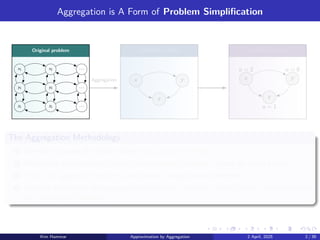
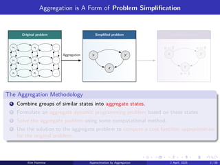
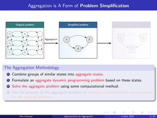
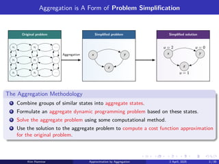
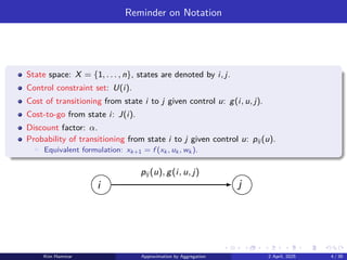
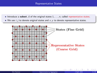
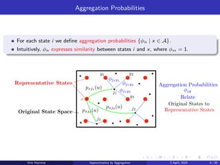
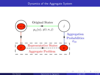
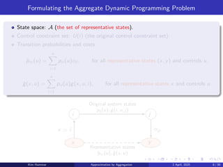
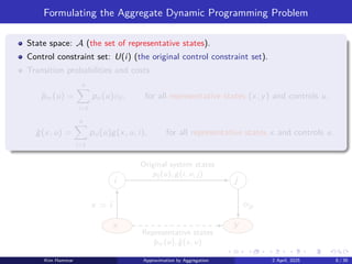
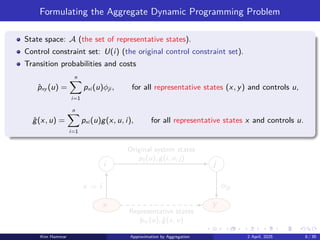
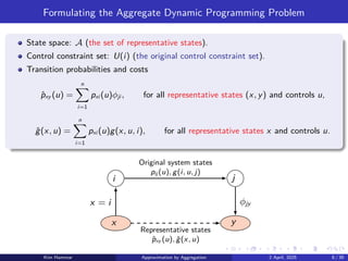
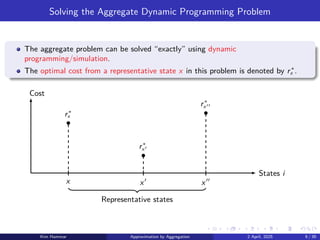
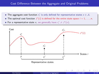
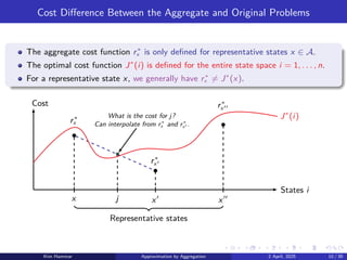
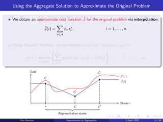
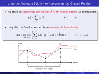

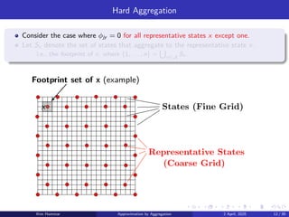
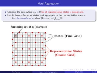
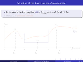
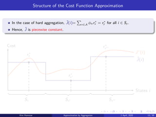
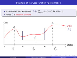
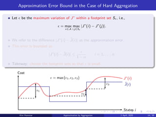
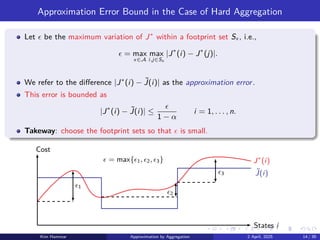
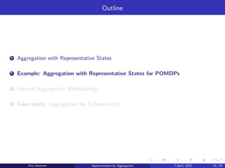
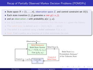
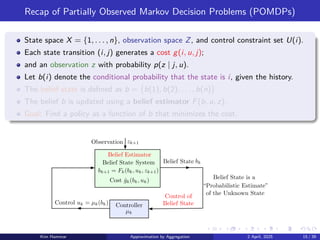
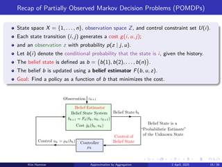

![The Belief Space
The belief b resides in the belief space B, i.e., the n − 1 dimensional unit simplex.
For example, if the states are {0, 1}, then b ∈ [0, 1].
(b) 2-dimensional unit simplex.
0.25 0.55
0.2
(1, 0, 0) (0, 1, 0)
(0, 0, 1)
(0.25, 0.55, 0.2)
(a) 1-dimensional unit simplex.
(1, 0) (0, 1)
0.4 0.6
(0.4, 0.6)
Kim Hammar Approximation by Aggregation 2 April, 2025 16 / 39](https://image.slidesharecdn.com/asuaggregationlecture2april2025-250403033056-b94b1c1e/85/Approximation-in-Value-Space-using-Aggregation-with-Applications-to-POMDPs-and-Cybersecurity-36-320.jpg)
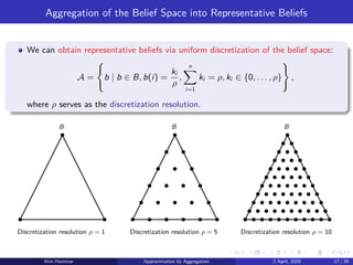


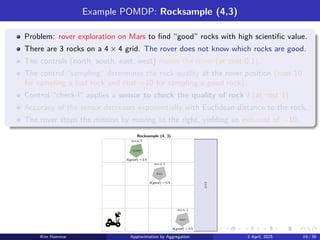
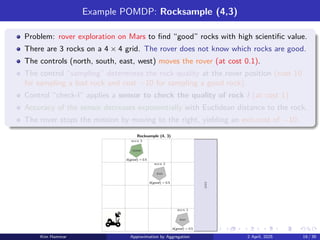
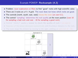
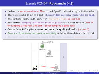
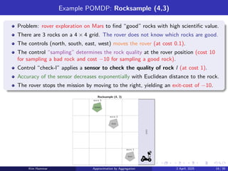
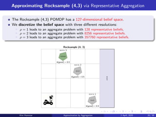
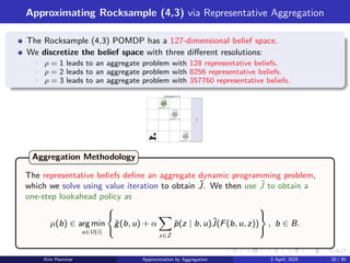

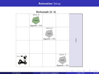
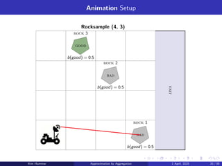


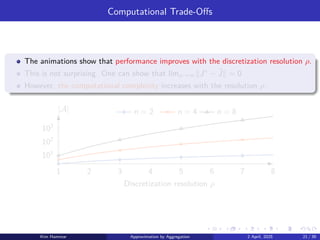
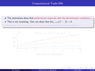
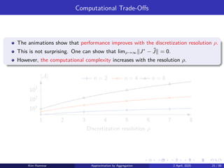
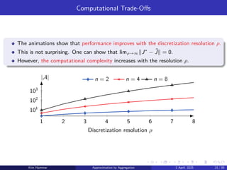
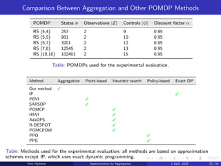
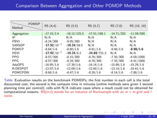

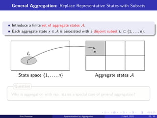
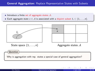
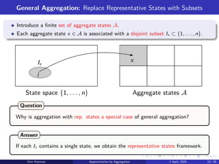
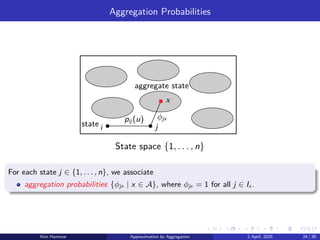
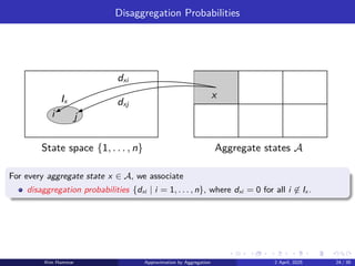
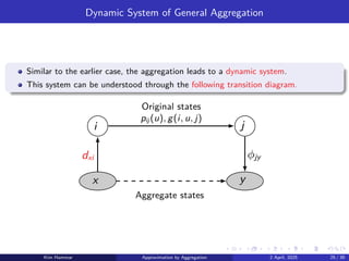
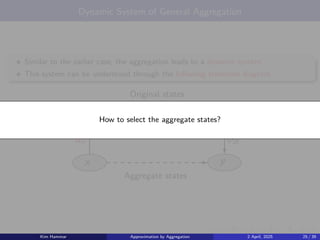
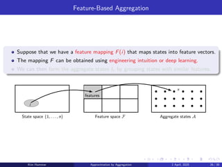
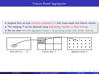
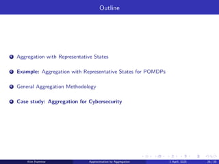

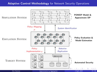
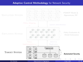
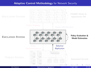
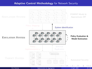
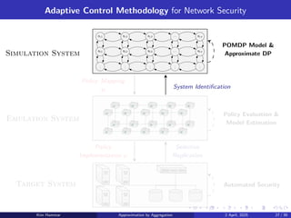
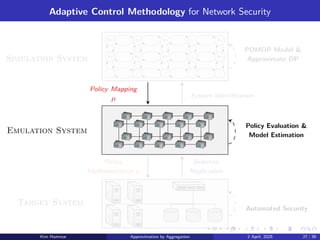
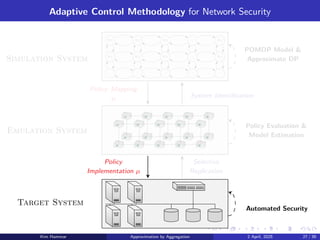
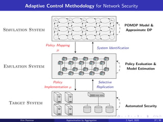
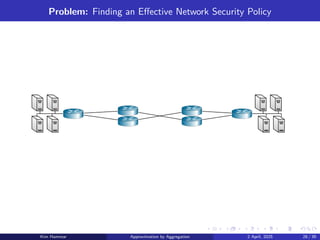
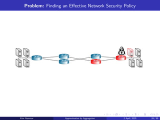
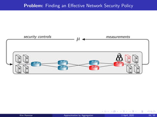
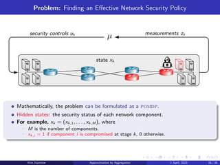
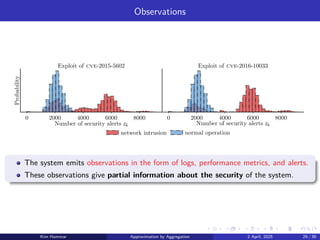
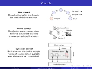
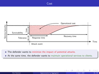
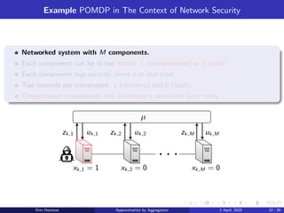
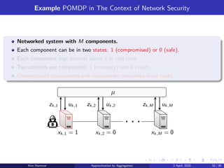
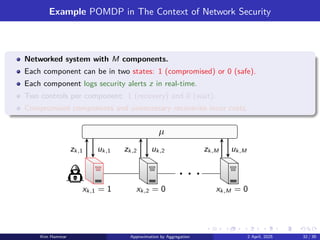
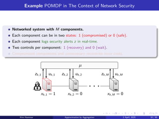
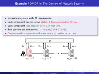
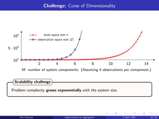
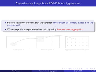
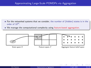


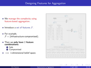
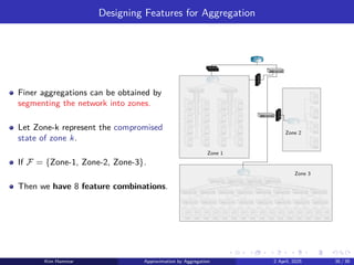
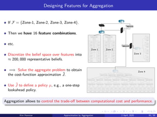
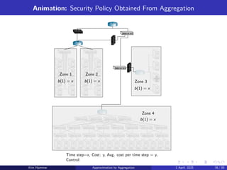
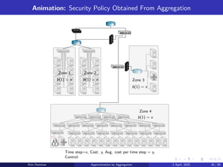

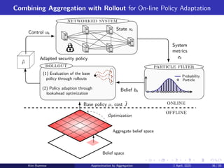
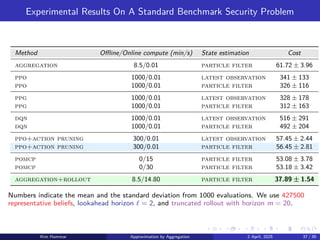
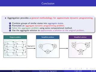


![5G Explained! A High Level Overview [Introduction]](https://cdn.slidesharecdn.com/ss_thumbnails/5gexplainedahighleveloverview-260119165306-cc137a3e-thumbnail.jpg?width=640&height=640&fit=bounds)


