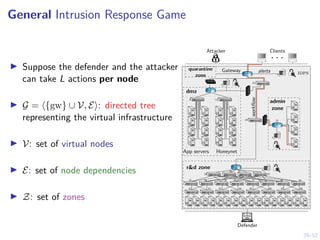
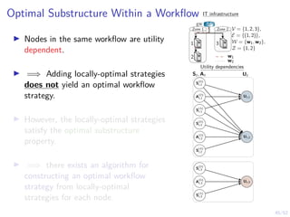
Download to read offline


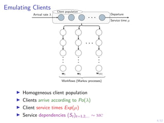

![19/52
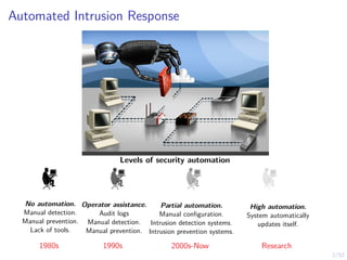
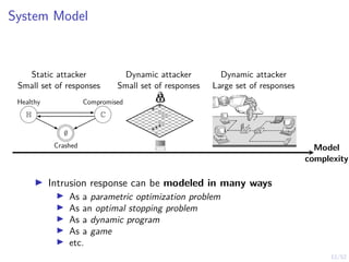
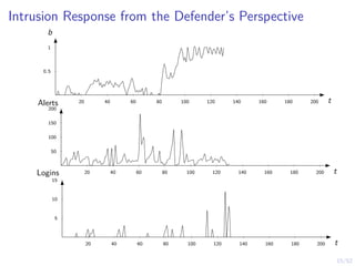
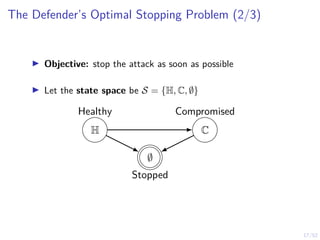
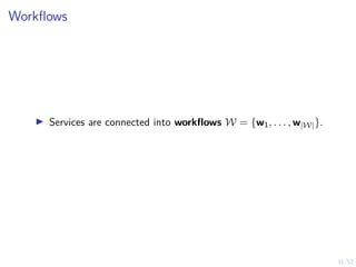
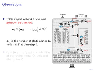
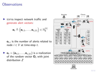
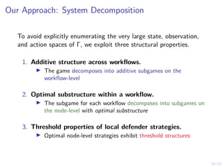
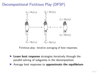
Optimal Stopping Strategy
I The defender can compute the belief
bt , P[Si,t = C | b1, o1, o2, . . . ot]
I Stopping strategy: π(b) : [0, 1] → {S, C}](https://image.slidesharecdn.com/hammarericssonresearchdec2023-231208130205-8fcc76b1/85/Learning-Automated-Intrusion-Response-38-320.jpg)
![19/52
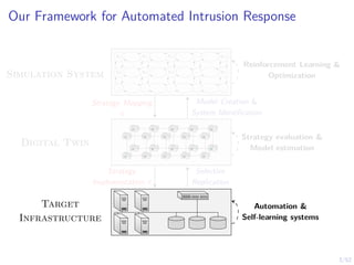
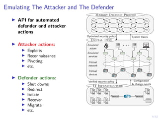
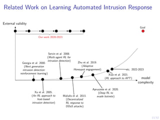
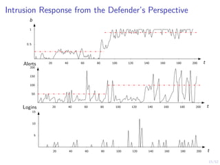
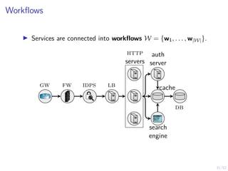
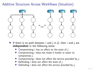
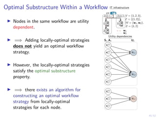
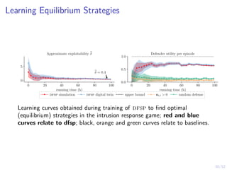
Optimal Threshold Strategy
Theorem
There exists an optimal defender strategy of the form:
π?
(b) = S ⇐⇒ b ≥ α?
α?
∈ [0, 1]
i.e., the stopping set is S = [α?, 1]
b
0 1
belief space B = [0, 1]
S1
α?
1](https://image.slidesharecdn.com/hammarericssonresearchdec2023-231208130205-8fcc76b1/85/Learning-Automated-Intrusion-Response-39-320.jpg)
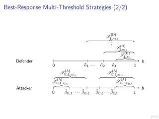
![21/52
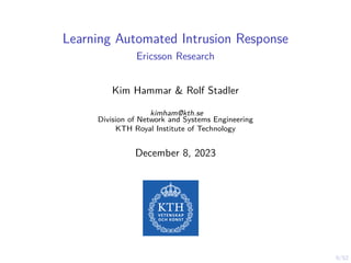
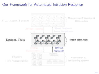
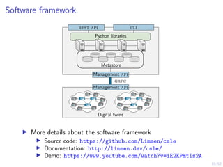
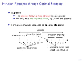
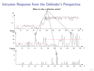
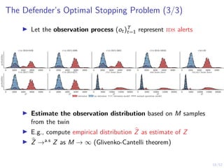
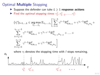
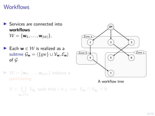
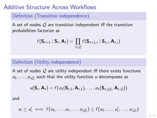
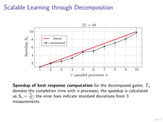
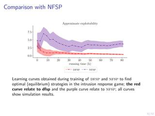
Optimal Multi-Threshold Strategy
Theorem
I Stopping sets are nested Sl−1 ⊆ Sl for l = 2, . . . L.
I If (ot)t≥1 is totally positive of order 2 (TP2), there exists an
optimal defender strategy of the form:
π?
l (b) = S ⇐⇒ b ≥ α?
l , l = 1, . . . , L
where α?
l ∈ [0, 1] is decreasing in l.
b
0 1
belief space B = [0, 1]
S1
S2
.
.
.
SL
α?
1
α?
2
α?
L
. . .](https://image.slidesharecdn.com/hammarericssonresearchdec2023-231208130205-8fcc76b1/85/Learning-Automated-Intrusion-Response-41-320.jpg)
![22/52
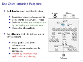
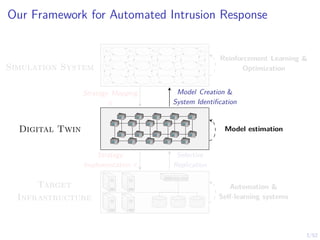
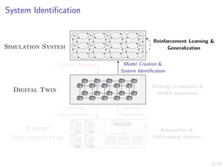
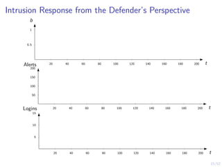
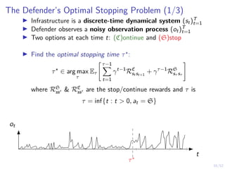
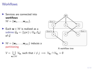
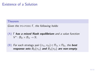
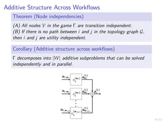
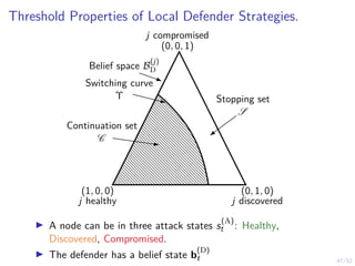
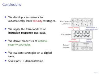
Optimal Stopping Game
I Suppose the attacker is dynamic and decides when to start
and abort its intrusion.
Attacker
Defender
t = 1
t = T
τ1,1 τ1,2 τ1,3
τ2,1
t
Stopped
Game episode
Intrusion
I Find the optimal stopping times
maximize
τD,1,...,τD,L
minimize
τA,1,τA,2
E[J]
where J is the defender’s objective.](https://image.slidesharecdn.com/hammarericssonresearchdec2023-231208130205-8fcc76b1/85/Learning-Automated-Intrusion-Response-42-320.jpg)
![25/52
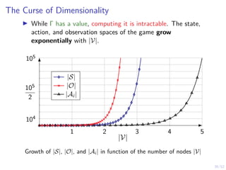
Efficient Computation of Best Responses
Algorithm 1: Threshold Optimization
1 Input: Objective function J, number of thresholds L,
parametric optimizer PO
2 Output: A approximate best response strategy π̂θ
3 Algorithm
4 Θ ← [0, 1]L
5 For each θ ∈ Θ, define πθ(bt) as
6 πθ(bt) ,
(
S if bt ≥ θi
C otherwise
7 Jθ ← Eπθ
[J]
8 π̂θ ← PO(Θ, Jθ)
9 return π̂θ
I Examples of parameteric optimization algorithmns: CEM, BO,
CMA-ES, DE, SPSA, etc.](https://image.slidesharecdn.com/hammarericssonresearchdec2023-231208130205-8fcc76b1/85/Learning-Automated-Intrusion-Response-45-320.jpg)
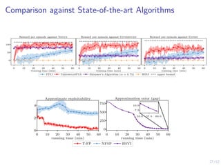
![28/52
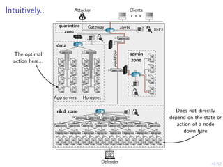
Learning Curves in Simulation and Digital Twin
0
50
100
Novice
Reward per episode
0
50
100
Episode length (steps)
0.0
0.5
1.0
P[intrusion interrupted]
0.0
0.5
1.0
1.5
P[early stopping]
5
10
Duration of intrusion
−50
0
50
100
experienced
0
50
100
150
0.0
0.5
1.0
0.0
0.5
1.0
1.5
0
5
10
0 20 40 60
training time (min)
−50
0
50
100
expert
0 20 40 60
training time (min)
0
50
100
150
0 20 40 60
training time (min)
0.0
0.5
1.0
0 20 40 60
training time (min)
0.0
0.5
1.0
1.5
2.0
0 20 40 60
training time (min)
0
5
10
15
20
πθ,l simulation πθ,l emulation (∆x + ∆y) ≥ 1 baseline Snort IPS upper bound
0 20 40 60 80 100
# training iterations
0
1
2
3
Exploitability
0 20 40 60 80 100
# training iterations
−5.0
−2.5
0.0
2.5
5.0
Defender reward per episode
0 20 40 60 80 100
# training iterations
0
1
2
3
Intrusion length
(π1,l, π2,l) emulation (π1,l, π2,l) simulation Snort IPS ot ≥ 1 upper bound](https://image.slidesharecdn.com/hammarericssonresearchdec2023-231208130205-8fcc76b1/85/Learning-Automated-Intrusion-Response-48-320.jpg)
![28/52
Learning Curves in Simulation and Digital Twin
0
50
100
Novice
Reward per episode
0
50
100
Episode length (steps)
0.0
0.5
1.0
P[intrusion interrupted]
0.0
0.5
1.0
1.5
P[early stopping]
5
10
Duration of intrusion
−50
0
50
100
experienced
0
50
100
150
0.0
0.5
1.0
0.0
0.5
1.0
1.5
0
5
10
0 20 40 60
training time (min)
−50
0
50
100
expert
0 20 40 60
training time (min)
0
50
100
150
0 20 40 60
training time (min)
0.0
0.5
1.0
0 20 40 60
training time (min)
0.0
0.5
1.0
1.5
2.0
0 20 40 60
training time (min)
0
5
10
15
20
πθ,l simulation πθ,l emulation (∆x + ∆y) ≥ 1 baseline Snort IPS upper bound
0 20 40 60 80 100
# training iterations
0
1
2
3
Exploitability
0 20 40 60 80 100
# training iterations
−5.0
−2.5
0.0
2.5
5.0
Defender reward per episode
0 20 40 60 80 100
# training iterations
0
1
2
3
Intrusion length
(π1,l, π2,l) emulation (π1,l, π2,l) simulation Snort IPS ot ≥ 1 upper bound
Stopping is about timing; now we consider timing + action selection](https://image.slidesharecdn.com/hammarericssonresearchdec2023-231208130205-8fcc76b1/85/Learning-Automated-Intrusion-Response-49-320.jpg)
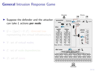

![37/52
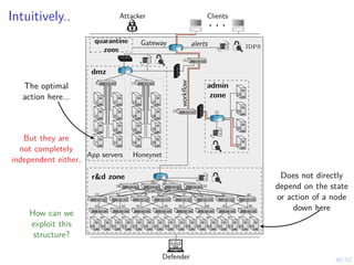
The Intrusion Response Problem
maximize
πD∈ΠD
minimize
πA∈ΠA
E(πD,πA) [J]
subject to s
(D)
t+1 ∼ fD · | A
(D)
t , A
(D)
t
∀t
s
(A)
t+1 ∼ fA · | S
(A)
t , At
∀t
ot+1 ∼ Z · | S
(D)
t+1, A
(A)
t ) ∀t
a
(A)
t ∼ πA · | H
(A)
t
, a
(A)
t ∈ AA(st) ∀t
a
(D)
t ∼ πD · | H
(D)
t
, a
(D)
t ∈ AD ∀t
E(πD,πA) denotes the expectation of the random vectors
(St, Ot, At)t∈{1,...,T} when following the strategy profile (πD, πA)
(1) can be formulated as a zero-sum Partially Observed Stochastic
Game with Public Observations (a PO-POSG):
Γ = hN, (Si )i∈N , (Ai )i∈N , (fi )i∈N , u, γ, (b
(i)
1 )i∈N , O, Zi](https://image.slidesharecdn.com/hammarericssonresearchdec2023-231208130205-8fcc76b1/85/Learning-Automated-Intrusion-Response-68-320.jpg)


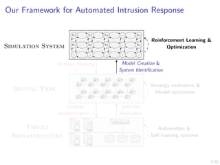
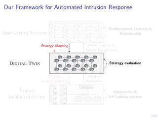
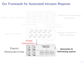
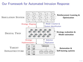
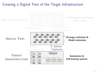
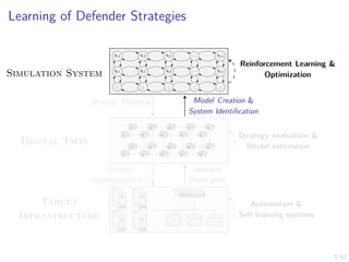
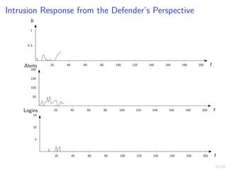
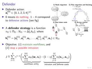
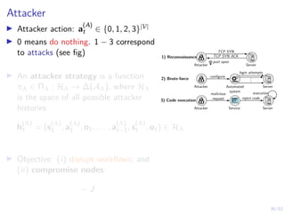
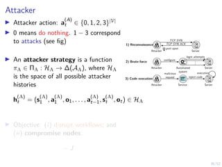
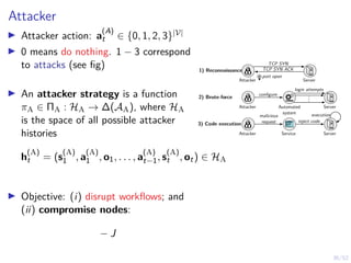
The document discusses a framework for automated intrusion response using reinforcement learning. It involves creating a digital twin of the target infrastructure, learning defender strategies through simulation, and evaluating strategies. The goal is to develop self-learning systems that can optimize intrusion response over time as attacks evolve.