Download as PDF, PPTX


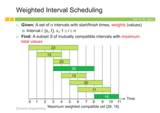
![IRIS H.-R. JIANG
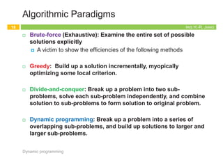
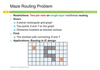
Designing a Recursive Algorithm (2/3)
¨ Second attempt: Induction on interval index
¤ First of all, sort intervals in ascending order of finish times
¤ In fact, this is also a trick for DP
¨ p(j) is the largest index i < j s.t. intervals i and j are disjoint
¤ p(j) = 0 if no request i < j is disjoint from j
Dynamic programming
9
1
2
2
4
4
7
p(1) = 0
p(2) = 0
p(3) = 1
p(4) = 0
p(5) = 3
p(6) = 3
1
2
3
4
5
6
p(2) = 0
p(6) = 3
4
1
4
IRIS H.-R. JIANG
Designing a Recursive Algorithm (3/3)
¨ Oj = the optimal solution for intervals 1, …, j
¨ OPT(j) = the value of the optimal solution for intervals 1, …, j
¤ e.g., O6 = ? Include interval 6 or not?
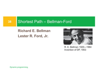
n Þ O6 = {6, O3} or O5
n OPT(6) = max{{v6+OPT(3)}, OPT(5)}
¤ OPT(j) = max{{vj+OPT(p(j))}, OPT(j-1)}
Dynamic programming
10
1
2
2
4
4
7
p(1) = 0
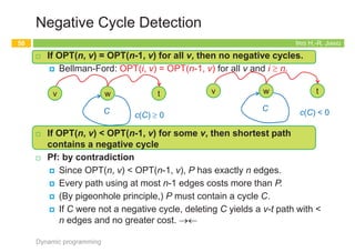
p(2) = 0
p(3) = 1
p(4) = 0
p(5) = 3
p(6) = 3
1
2
3
4
5
6 1
IRIS H.-R. JIANG
Direct Implementation
Dynamic programming
11
// Preprocessing:
// 1. Sort intervals by finish times: f1 £ f2 £ ... £ fn
// 2. Compute p(1), p(2), …, p(n)
Compute-Opt(j)
1. if (j = 0) then return 0
2. else return max{{vj+Compute-Opt(p(j))}, Compute-Opt(j-1)}
OPT(j) = max{{vj+OPT(p(j))}, OPT(j-1)}
5
4
3
1
2
1
3
2 1
1
6
3
2 1
1
The tree of calls widens very quickly
due to recursive branching!
1
2
2
4
4
7
p(1) = 0
p(2) = 0
p(3) = 1
p(4) = 0
p(5) = 3
p(6) = 3
IRIS H.-R. JIANG
Memoization: Top-Down
¨ The tree of calls widens very quickly due to recursive
branching!
¤ e.g., exponential running time when p(j) = j – 2 for all j
¨ Q: What’s wrong? A: Redundant calls!
¨ Q: How to eliminate this redundancy?
¨ A: Store the value for future! (memoization)
Dynamic programming
12
5
4
3
1
2
1
3
2 1
1
6
3
2 1
1
3
1
2
1
3
2 1
1
3
2 1
1
M-Compute-Opt(j)
1. if (j = 0) then return 0
2. else if (M[j] is not empty) then return M[j]
3. else return M[j] = max{{vj+M-Compute-Opt(p(j))},
M-Compute-Opt(j-1)}
Running time:
O(n)
How to report the
optimal solution O?
5
4
3
2
1
6](https://image.slidesharecdn.com/algorithm6dynamicprogramming-220522073057-711c84d9/85/algorithm_6dynamic_programming-pdf-9-320.jpg)
![IRIS H.-R. JIANG
Designing a Recursive Algorithm (2/3)
¨ Second attempt: Induction on interval index
¤ First of all, sort intervals in ascending order of finish times
¤ In fact, this is also a trick for DP
¨ p(j) is the largest index i < j s.t. intervals i and j are disjoint
¤ p(j) = 0 if no request i < j is disjoint from j
Dynamic programming
9
1
2
2
4
4
7
p(1) = 0
p(2) = 0
p(3) = 1
p(4) = 0
p(5) = 3
p(6) = 3
1
2
3
4
5
6
p(2) = 0
p(6) = 3
4
1
4
IRIS H.-R. JIANG
Designing a Recursive Algorithm (3/3)
¨ Oj = the optimal solution for intervals 1, …, j
¨ OPT(j) = the value of the optimal solution for intervals 1, …, j
¤ e.g., O6 = ? Include interval 6 or not?
n Þ O6 = {6, O3} or O5
n OPT(6) = max{{v6+OPT(3)}, OPT(5)}
¤ OPT(j) = max{{vj+OPT(p(j))}, OPT(j-1)}
Dynamic programming
10
1
2
2
4
4
7
p(1) = 0
p(2) = 0
p(3) = 1
p(4) = 0
p(5) = 3
p(6) = 3
1
2
3
4
5
6 1
IRIS H.-R. JIANG
Direct Implementation
Dynamic programming
11
// Preprocessing:
// 1. Sort intervals by finish times: f1 £ f2 £ ... £ fn
// 2. Compute p(1), p(2), …, p(n)
Compute-Opt(j)
1. if (j = 0) then return 0
2. else return max{{vj+Compute-Opt(p(j))}, Compute-Opt(j-1)}
OPT(j) = max{{vj+OPT(p(j))}, OPT(j-1)}
5
4
3
1
2
1
3
2 1
1
6
3
2 1
1
The tree of calls widens very quickly
due to recursive branching!
1
2
2
4
4
7
p(1) = 0
p(2) = 0
p(3) = 1
p(4) = 0
p(5) = 3
p(6) = 3
IRIS H.-R. JIANG
Memoization: Top-Down
¨ The tree of calls widens very quickly due to recursive
branching!
¤ e.g., exponential running time when p(j) = j – 2 for all j
¨ Q: What’s wrong? A: Redundant calls!
¨ Q: How to eliminate this redundancy?
¨ A: Store the value for future! (memoization)
Dynamic programming
12
5
4
3
1
2
1
3
2 1
1
6
3
2 1
1
3
1
2
1
3
2 1
1
3
2 1
1
M-Compute-Opt(j)
1. if (j = 0) then return 0
2. else if (M[j] is not empty) then return M[j]
3. else return M[j] = max{{vj+M-Compute-Opt(p(j))},
M-Compute-Opt(j-1)}
Running time:
O(n)
How to report the
optimal solution O?
5
4
3
2
1
6](https://image.slidesharecdn.com/algorithm6dynamicprogramming-220522073057-711c84d9/85/algorithm_6dynamic_programming-pdf-10-320.jpg)
![IRIS H.-R. JIANG
Designing a Recursive Algorithm (2/3)
¨ Second attempt: Induction on interval index
¤ First of all, sort intervals in ascending order of finish times
¤ In fact, this is also a trick for DP
¨ p(j) is the largest index i < j s.t. intervals i and j are disjoint
¤ p(j) = 0 if no request i < j is disjoint from j
Dynamic programming
9
1
2
2
4
4
7
p(1) = 0
p(2) = 0
p(3) = 1
p(4) = 0
p(5) = 3
p(6) = 3
1
2
3
4
5
6
p(2) = 0
p(6) = 3
4
1
4
IRIS H.-R. JIANG
Designing a Recursive Algorithm (3/3)
¨ Oj = the optimal solution for intervals 1, …, j
¨ OPT(j) = the value of the optimal solution for intervals 1, …, j
¤ e.g., O6 = ? Include interval 6 or not?
n Þ O6 = {6, O3} or O5
n OPT(6) = max{{v6+OPT(3)}, OPT(5)}
¤ OPT(j) = max{{vj+OPT(p(j))}, OPT(j-1)}
Dynamic programming
10
1
2
2
4
4
7
p(1) = 0
p(2) = 0
p(3) = 1
p(4) = 0
p(5) = 3
p(6) = 3
1
2
3
4
5
6 1
IRIS H.-R. JIANG
Direct Implementation
Dynamic programming
11
// Preprocessing:
// 1. Sort intervals by finish times: f1 £ f2 £ ... £ fn
// 2. Compute p(1), p(2), …, p(n)
Compute-Opt(j)
1. if (j = 0) then return 0
2. else return max{{vj+Compute-Opt(p(j))}, Compute-Opt(j-1)}
OPT(j) = max{{vj+OPT(p(j))}, OPT(j-1)}
5
4
3
1
2
1
3
2 1
1
6
3
2 1
1
The tree of calls widens very quickly
due to recursive branching!
1
2
2
4
4
7
p(1) = 0
p(2) = 0
p(3) = 1
p(4) = 0
p(5) = 3
p(6) = 3
IRIS H.-R. JIANG
Memoization: Top-Down
¨ The tree of calls widens very quickly due to recursive
branching!
¤ e.g., exponential running time when p(j) = j – 2 for all j
¨ Q: What’s wrong? A: Redundant calls!
¨ Q: How to eliminate this redundancy?
¨ A: Store the value for future! (memoization)
Dynamic programming
12
5
4
3
1
2
1
3
2 1
1
6
3
2 1
1
3
1
2
1
3
2 1
1
3
2 1
1
M-Compute-Opt(j)
1. if (j = 0) then return 0
2. else if (M[j] is not empty) then return M[j]
3. else return M[j] = max{{vj+M-Compute-Opt(p(j))},
M-Compute-Opt(j-1)}
Running time:
O(n)
How to report the
optimal solution O?
5
4
3
2
1
6](https://image.slidesharecdn.com/algorithm6dynamicprogramming-220522073057-711c84d9/85/algorithm_6dynamic_programming-pdf-11-320.jpg)
![IRIS H.-R. JIANG
Designing a Recursive Algorithm (2/3)
¨ Second attempt: Induction on interval index
¤ First of all, sort intervals in ascending order of finish times
¤ In fact, this is also a trick for DP
¨ p(j) is the largest index i < j s.t. intervals i and j are disjoint
¤ p(j) = 0 if no request i < j is disjoint from j
Dynamic programming
9
1
2
2
4
4
7
p(1) = 0
p(2) = 0
p(3) = 1
p(4) = 0
p(5) = 3
p(6) = 3
1
2
3
4
5
6
p(2) = 0
p(6) = 3
4
1
4
IRIS H.-R. JIANG
Designing a Recursive Algorithm (3/3)
¨ Oj = the optimal solution for intervals 1, …, j
¨ OPT(j) = the value of the optimal solution for intervals 1, …, j
¤ e.g., O6 = ? Include interval 6 or not?
n Þ O6 = {6, O3} or O5
n OPT(6) = max{{v6+OPT(3)}, OPT(5)}
¤ OPT(j) = max{{vj+OPT(p(j))}, OPT(j-1)}
Dynamic programming
10
1
2
2
4
4
7
p(1) = 0
p(2) = 0
p(3) = 1
p(4) = 0
p(5) = 3
p(6) = 3
1
2
3
4
5
6 1
IRIS H.-R. JIANG
Direct Implementation
Dynamic programming
11
// Preprocessing:
// 1. Sort intervals by finish times: f1 £ f2 £ ... £ fn
// 2. Compute p(1), p(2), …, p(n)
Compute-Opt(j)
1. if (j = 0) then return 0
2. else return max{{vj+Compute-Opt(p(j))}, Compute-Opt(j-1)}
OPT(j) = max{{vj+OPT(p(j))}, OPT(j-1)}
5
4
3
1
2
1
3
2 1
1
6
3
2 1
1
The tree of calls widens very quickly
due to recursive branching!
1
2
2
4
4
7
p(1) = 0
p(2) = 0
p(3) = 1
p(4) = 0
p(5) = 3
p(6) = 3
IRIS H.-R. JIANG
Memoization: Top-Down
¨ The tree of calls widens very quickly due to recursive
branching!
¤ e.g., exponential running time when p(j) = j – 2 for all j
¨ Q: What’s wrong? A: Redundant calls!
¨ Q: How to eliminate this redundancy?
¨ A: Store the value for future! (memoization)
Dynamic programming
12
5
4
3
1
2
1
3
2 1
1
6
3
2 1
1
3
1
2
1
3
2 1
1
3
2 1
1
M-Compute-Opt(j)
1. if (j = 0) then return 0
2. else if (M[j] is not empty) then return M[j]
3. else return M[j] = max{{vj+M-Compute-Opt(p(j))},
M-Compute-Opt(j-1)}
Running time:
O(n)
How to report the
optimal solution O?
5
4
3
2
1
6](https://image.slidesharecdn.com/algorithm6dynamicprogramming-220522073057-711c84d9/85/algorithm_6dynamic_programming-pdf-12-320.jpg)
![IRIS H.-R. JIANG
Iteration: Bottom-Up
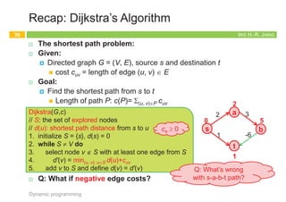
¨ We can also compute the array M[j] by an iterative algorithm.
Dynamic programming
13
I-Compute-Opt
1. M[0] = 0
2. for j = 1, 2, .., n do
3. M[j] = max{vj+M[p(j)], M[j-1]}
Running time:
O(n)
1
2
2
4
4
7
p(1) = 0
p(2) = 0
p(3) = 1
p(4) = 0
p(5) = 3
p(6) = 3
1
2
3
4
5
6
0 2 4
0 2 4 6
0 2 4 6 7
0 2 4 6 7 8
0 2 4 6 7 8 8
M =
0 1 2 3 4 5
0
6
0 2
max{4+0, 2}
IRIS H.-R. JIANG
Summary: Memoization vs. Iteration
¨ Top-down
¨ An recursive algorithm
¤ Compute only what we need
¨ Bottom-up
¨ An iterative algorithm
¤ Construct solutions from the
smallest subproblem to the
largest one
¤ Compute every small piece
Memoization Iteration
14
Dynamic programming
The running time and
memory requirement highly
depend on the table size
Start with the recursive
divide-and-conquer
algorithm
IRIS H.-R. JIANG
Keys for Dynamic Programming
¨ Dynamic programming can be used if the problem satisfies the
following properties:
¤ There are only a polynomial number of subproblems
¤ The solution to the original problem can be easily computed from
the solutions to the subproblems
¤ There is a natural ordering on subproblems from “smallest” to
“largest,” together with an easy-to-compute recurrence
Dynamic programming
15
5
4
3
1
2
1
3
2 1
1
6
3
2 1
1
3
1
2
1
3
2 1
1
3
2 1
1
5
4
3
2
1
6
IRIS H.-R. JIANG
Keys for Dynamic Programming
¨ DP typically is applied to optimization problems.
¨ DP works best on objects that are linearly ordered an cannot be
rearranged
¨ Elements of DP
¤ Optimal substructure: an optimal solution contains within its
optimal solutions to subproblems.
¤ Overlapping subproblem: a recursive algorithm revisits the same
problem over and over again; typically, the total number of distinct
subproblems is a polynomial in the input size.
Dynamic programming
16
Cormen, Leiserson, Rivest, Stein, Introduction to Algorithms,
2nd Ed., McGraw Hill/MIT Press, 2001
5
4
3
1
2
1
3
2 1
1
6
3
2 1
1
3
1
2
1
3
2 1
1
3
2 1
1
5
4
3
2
1
6
In optimization problems, we
are interested in finding a thing
which maximizes or minimizes
some function.](https://image.slidesharecdn.com/algorithm6dynamicprogramming-220522073057-711c84d9/85/algorithm_6dynamic_programming-pdf-13-320.jpg)
![IRIS H.-R. JIANG
Iteration: Bottom-Up
¨ We can also compute the array M[j] by an iterative algorithm.
Dynamic programming
13
I-Compute-Opt
1. M[0] = 0
2. for j = 1, 2, .., n do
3. M[j] = max{vj+M[p(j)], M[j-1]}
Running time:
O(n)
1
2
2
4
4
7
p(1) = 0
p(2) = 0
p(3) = 1
p(4) = 0
p(5) = 3
p(6) = 3
1
2
3
4
5
6
0 2 4
0 2 4 6
0 2 4 6 7
0 2 4 6 7 8
0 2 4 6 7 8 8
M =
0 1 2 3 4 5
0
6
0 2
max{4+0, 2}
IRIS H.-R. JIANG
Summary: Memoization vs. Iteration
¨ Top-down
¨ An recursive algorithm
¤ Compute only what we need
¨ Bottom-up
¨ An iterative algorithm
¤ Construct solutions from the
smallest subproblem to the
largest one
¤ Compute every small piece
Memoization Iteration
14
Dynamic programming
The running time and
memory requirement highly
depend on the table size
Start with the recursive
divide-and-conquer
algorithm
IRIS H.-R. JIANG
Keys for Dynamic Programming
¨ Dynamic programming can be used if the problem satisfies the
following properties:
¤ There are only a polynomial number of subproblems
¤ The solution to the original problem can be easily computed from
the solutions to the subproblems
¤ There is a natural ordering on subproblems from “smallest” to
“largest,” together with an easy-to-compute recurrence
Dynamic programming
15
5
4
3
1
2
1
3
2 1
1
6
3
2 1
1
3
1
2
1
3
2 1
1
3
2 1
1
5
4
3
2
1
6
IRIS H.-R. JIANG
Keys for Dynamic Programming
¨ DP typically is applied to optimization problems.
¨ DP works best on objects that are linearly ordered an cannot be
rearranged
¨ Elements of DP
¤ Optimal substructure: an optimal solution contains within its
optimal solutions to subproblems.
¤ Overlapping subproblem: a recursive algorithm revisits the same
problem over and over again; typically, the total number of distinct
subproblems is a polynomial in the input size.
Dynamic programming
16
Cormen, Leiserson, Rivest, Stein, Introduction to Algorithms,
2nd Ed., McGraw Hill/MIT Press, 2001
5
4
3
1
2
1
3
2 1
1
6
3
2 1
1
3
1
2
1
3
2 1
1
3
2 1
1
5
4
3
2
1
6
In optimization problems, we
are interested in finding a thing
which maximizes or minimizes
some function.](https://image.slidesharecdn.com/algorithm6dynamicprogramming-220522073057-711c84d9/85/algorithm_6dynamic_programming-pdf-14-320.jpg)
![IRIS H.-R. JIANG
Iteration: Bottom-Up
¨ We can also compute the array M[j] by an iterative algorithm.
Dynamic programming
13
I-Compute-Opt
1. M[0] = 0
2. for j = 1, 2, .., n do
3. M[j] = max{vj+M[p(j)], M[j-1]}
Running time:
O(n)
1
2
2
4
4
7
p(1) = 0
p(2) = 0
p(3) = 1
p(4) = 0
p(5) = 3
p(6) = 3
1
2
3
4
5
6
0 2 4
0 2 4 6
0 2 4 6 7
0 2 4 6 7 8
0 2 4 6 7 8 8
M =
0 1 2 3 4 5
0
6
0 2
max{4+0, 2}
IRIS H.-R. JIANG
Summary: Memoization vs. Iteration
¨ Top-down
¨ An recursive algorithm
¤ Compute only what we need
¨ Bottom-up
¨ An iterative algorithm
¤ Construct solutions from the
smallest subproblem to the
largest one
¤ Compute every small piece
Memoization Iteration
14
Dynamic programming
The running time and
memory requirement highly
depend on the table size
Start with the recursive
divide-and-conquer
algorithm
IRIS H.-R. JIANG
Keys for Dynamic Programming
¨ Dynamic programming can be used if the problem satisfies the
following properties:
¤ There are only a polynomial number of subproblems
¤ The solution to the original problem can be easily computed from
the solutions to the subproblems
¤ There is a natural ordering on subproblems from “smallest” to
“largest,” together with an easy-to-compute recurrence
Dynamic programming
15
5
4
3
1
2
1
3
2 1
1
6
3
2 1
1
3
1
2
1
3
2 1
1
3
2 1
1
5
4
3
2
1
6
IRIS H.-R. JIANG
Keys for Dynamic Programming
¨ DP typically is applied to optimization problems.
¨ DP works best on objects that are linearly ordered an cannot be
rearranged
¨ Elements of DP
¤ Optimal substructure: an optimal solution contains within its
optimal solutions to subproblems.
¤ Overlapping subproblem: a recursive algorithm revisits the same
problem over and over again; typically, the total number of distinct
subproblems is a polynomial in the input size.
Dynamic programming
16
Cormen, Leiserson, Rivest, Stein, Introduction to Algorithms,
2nd Ed., McGraw Hill/MIT Press, 2001
5
4
3
1
2
1
3
2 1
1
6
3
2 1
1
3
1
2
1
3
2 1
1
3
2 1
1
5
4
3
2
1
6
In optimization problems, we
are interested in finding a thing
which maximizes or minimizes
some function.](https://image.slidesharecdn.com/algorithm6dynamicprogramming-220522073057-711c84d9/85/algorithm_6dynamic_programming-pdf-15-320.jpg)
![IRIS H.-R. JIANG
Iteration: Bottom-Up
¨ We can also compute the array M[j] by an iterative algorithm.
Dynamic programming
13
I-Compute-Opt
1. M[0] = 0
2. for j = 1, 2, .., n do
3. M[j] = max{vj+M[p(j)], M[j-1]}
Running time:
O(n)
1
2
2
4
4
7
p(1) = 0
p(2) = 0
p(3) = 1
p(4) = 0
p(5) = 3
p(6) = 3
1
2
3
4
5
6
0 2 4
0 2 4 6
0 2 4 6 7
0 2 4 6 7 8
0 2 4 6 7 8 8
M =
0 1 2 3 4 5
0
6
0 2
max{4+0, 2}
IRIS H.-R. JIANG
Summary: Memoization vs. Iteration
¨ Top-down
¨ An recursive algorithm
¤ Compute only what we need
¨ Bottom-up
¨ An iterative algorithm
¤ Construct solutions from the
smallest subproblem to the
largest one
¤ Compute every small piece
Memoization Iteration
14
Dynamic programming
The running time and
memory requirement highly
depend on the table size
Start with the recursive
divide-and-conquer
algorithm
IRIS H.-R. JIANG
Keys for Dynamic Programming
¨ Dynamic programming can be used if the problem satisfies the
following properties:
¤ There are only a polynomial number of subproblems
¤ The solution to the original problem can be easily computed from
the solutions to the subproblems
¤ There is a natural ordering on subproblems from “smallest” to
“largest,” together with an easy-to-compute recurrence
Dynamic programming
15
5
4
3
1
2
1
3
2 1
1
6
3
2 1
1
3
1
2
1
3
2 1
1
3
2 1
1
5
4
3
2
1
6
IRIS H.-R. JIANG
Keys for Dynamic Programming
¨ DP typically is applied to optimization problems.
¨ DP works best on objects that are linearly ordered an cannot be
rearranged
¨ Elements of DP
¤ Optimal substructure: an optimal solution contains within its
optimal solutions to subproblems.
¤ Overlapping subproblem: a recursive algorithm revisits the same
problem over and over again; typically, the total number of distinct
subproblems is a polynomial in the input size.
Dynamic programming
16
Cormen, Leiserson, Rivest, Stein, Introduction to Algorithms,
2nd Ed., McGraw Hill/MIT Press, 2001
5
4
3
1
2
1
3
2 1
1
6
3
2 1
1
3
1
2
1
3
2 1
1
3
2 1
1
5
4
3
2
1
6
In optimization problems, we
are interested in finding a thing
which maximizes or minimizes
some function.](https://image.slidesharecdn.com/algorithm6dynamicprogramming-220522073057-711c84d9/85/algorithm_6dynamic_programming-pdf-16-320.jpg)
![IRIS H.-R. JIANG
What’s Wrong?
¨ What if we call fib(5)?
¤ fib(5)
¤ fib(4) + fib(3)
¤ (fib(3) + fib(2)) + (fib(2) + fib(1))
¤ ((fib(2) + fib(1)) + (fib(1) + fib(0))) + ((fib(1) + fib(0)) + fib(1))
¤ (((fib(1) + fib(0)) + fib(1))+(fib(1) + fib(0)))+((fib(1) + fib(0))+fib(1))
¤ A call tree that calls the function on the same value many
different times
n fib(2) was calculated three times from scratch
n Impractical for large n
Dynamic programming
21
fib(n)
1. if n £ 1 return n
2. return fib(n ! 1) + fib(n ! 2)
5
4
3
2
3
2 1
2
1 0 1 0
1
1 0
2
1 0
2
1 0
2
1 0
IRIS H.-R. JIANG
Too Many Redundant Calls!
¨ How to remove redundancy?
¤ Prevent repeated calculation
Recursion True dependency
Dynamic programming
22
5
4 3
2 1
5
4
3
2
3
2 1
2
1 0 1 0
1
1 0
3
2
3
1
2
1 0
1
1 0
2
1 0
2
1 0
2
1 0
IRIS H.-R. JIANG
Dynamic Programming -- Memoization
¨ Store the values in a table
¤ Check the table before a recursive call
¤ Top-down!
n The control flow is almost the same as the original one
Dynamic programming
23
fib(n)
1. Initialize f[0..n] with -1 // -1: unfilled
2. f[0] = 0; f[1] = 1
3. fibonacci(n, f)
fibonacci(n, f)
1. If f[n] == -1 then
2. f[n] = fibonacci(n ! 1, f) + fibonacci(n ! 2, f)
3. return f[n] // if f[n] already exists, directly return
5
4 3
2 1
IRIS H.-R. JIANG
Dynamic Programming -- Bottom-up?
¨ Store the values in a table
¤ Bottom-up
n Compute the values for small problems first
¤ Much like induction
Dynamic programming
24
fib(n)
1. initialize f[1..n] with -1 // -1: unfilled
2. f[0] = 0; f[1] = 1
3. for i=2 to n do
4. f[i] = f[i-1]+ f[i-2]
5. return f[n]
5
4 3
2 1](https://image.slidesharecdn.com/algorithm6dynamicprogramming-220522073057-711c84d9/85/algorithm_6dynamic_programming-pdf-21-320.jpg)
![IRIS H.-R. JIANG
What’s Wrong?
¨ What if we call fib(5)?
¤ fib(5)
¤ fib(4) + fib(3)
¤ (fib(3) + fib(2)) + (fib(2) + fib(1))
¤ ((fib(2) + fib(1)) + (fib(1) + fib(0))) + ((fib(1) + fib(0)) + fib(1))
¤ (((fib(1) + fib(0)) + fib(1))+(fib(1) + fib(0)))+((fib(1) + fib(0))+fib(1))
¤ A call tree that calls the function on the same value many
different times
n fib(2) was calculated three times from scratch
n Impractical for large n
Dynamic programming
21
fib(n)
1. if n £ 1 return n
2. return fib(n ! 1) + fib(n ! 2)
5
4
3
2
3
2 1
2
1 0 1 0
1
1 0
2
1 0
2
1 0
2
1 0
IRIS H.-R. JIANG
Too Many Redundant Calls!
¨ How to remove redundancy?
¤ Prevent repeated calculation
Recursion True dependency
Dynamic programming
22
5
4 3
2 1
5
4
3
2
3
2 1
2
1 0 1 0
1
1 0
3
2
3
1
2
1 0
1
1 0
2
1 0
2
1 0
2
1 0
IRIS H.-R. JIANG
Dynamic Programming -- Memoization
¨ Store the values in a table
¤ Check the table before a recursive call
¤ Top-down!
n The control flow is almost the same as the original one
Dynamic programming
23
fib(n)
1. Initialize f[0..n] with -1 // -1: unfilled
2. f[0] = 0; f[1] = 1
3. fibonacci(n, f)
fibonacci(n, f)
1. If f[n] == -1 then
2. f[n] = fibonacci(n ! 1, f) + fibonacci(n ! 2, f)
3. return f[n] // if f[n] already exists, directly return
5
4 3
2 1
IRIS H.-R. JIANG
Dynamic Programming -- Bottom-up?
¨ Store the values in a table
¤ Bottom-up
n Compute the values for small problems first
¤ Much like induction
Dynamic programming
24
fib(n)
1. initialize f[1..n] with -1 // -1: unfilled
2. f[0] = 0; f[1] = 1
3. for i=2 to n do
4. f[i] = f[i-1]+ f[i-2]
5. return f[n]
5
4 3
2 1](https://image.slidesharecdn.com/algorithm6dynamicprogramming-220522073057-711c84d9/85/algorithm_6dynamic_programming-pdf-22-320.jpg)
![IRIS H.-R. JIANG
What’s Wrong?
¨ What if we call fib(5)?
¤ fib(5)
¤ fib(4) + fib(3)
¤ (fib(3) + fib(2)) + (fib(2) + fib(1))
¤ ((fib(2) + fib(1)) + (fib(1) + fib(0))) + ((fib(1) + fib(0)) + fib(1))
¤ (((fib(1) + fib(0)) + fib(1))+(fib(1) + fib(0)))+((fib(1) + fib(0))+fib(1))
¤ A call tree that calls the function on the same value many
different times
n fib(2) was calculated three times from scratch
n Impractical for large n
Dynamic programming
21
fib(n)
1. if n £ 1 return n
2. return fib(n ! 1) + fib(n ! 2)
5
4
3
2
3
2 1
2
1 0 1 0
1
1 0
2
1 0
2
1 0
2
1 0
IRIS H.-R. JIANG
Too Many Redundant Calls!
¨ How to remove redundancy?
¤ Prevent repeated calculation
Recursion True dependency
Dynamic programming
22
5
4 3
2 1
5
4
3
2
3
2 1
2
1 0 1 0
1
1 0
3
2
3
1
2
1 0
1
1 0
2
1 0
2
1 0
2
1 0
IRIS H.-R. JIANG
Dynamic Programming -- Memoization
¨ Store the values in a table
¤ Check the table before a recursive call
¤ Top-down!
n The control flow is almost the same as the original one
Dynamic programming
23
fib(n)
1. Initialize f[0..n] with -1 // -1: unfilled
2. f[0] = 0; f[1] = 1
3. fibonacci(n, f)
fibonacci(n, f)
1. If f[n] == -1 then
2. f[n] = fibonacci(n ! 1, f) + fibonacci(n ! 2, f)
3. return f[n] // if f[n] already exists, directly return
5
4 3
2 1
IRIS H.-R. JIANG
Dynamic Programming -- Bottom-up?
¨ Store the values in a table
¤ Bottom-up
n Compute the values for small problems first
¤ Much like induction
Dynamic programming
24
fib(n)
1. initialize f[1..n] with -1 // -1: unfilled
2. f[0] = 0; f[1] = 1
3. for i=2 to n do
4. f[i] = f[i-1]+ f[i-2]
5. return f[n]
5
4 3
2 1](https://image.slidesharecdn.com/algorithm6dynamicprogramming-220522073057-711c84d9/85/algorithm_6dynamic_programming-pdf-23-320.jpg)
![IRIS H.-R. JIANG
What’s Wrong?
¨ What if we call fib(5)?
¤ fib(5)
¤ fib(4) + fib(3)
¤ (fib(3) + fib(2)) + (fib(2) + fib(1))
¤ ((fib(2) + fib(1)) + (fib(1) + fib(0))) + ((fib(1) + fib(0)) + fib(1))
¤ (((fib(1) + fib(0)) + fib(1))+(fib(1) + fib(0)))+((fib(1) + fib(0))+fib(1))
¤ A call tree that calls the function on the same value many
different times
n fib(2) was calculated three times from scratch
n Impractical for large n
Dynamic programming
21
fib(n)
1. if n £ 1 return n
2. return fib(n ! 1) + fib(n ! 2)
5
4
3
2
3
2 1
2
1 0 1 0
1
1 0
2
1 0
2
1 0
2
1 0
IRIS H.-R. JIANG
Too Many Redundant Calls!
¨ How to remove redundancy?
¤ Prevent repeated calculation
Recursion True dependency
Dynamic programming
22
5
4 3
2 1
5
4
3
2
3
2 1
2
1 0 1 0
1
1 0
3
2
3
1
2
1 0
1
1 0
2
1 0
2
1 0
2
1 0
IRIS H.-R. JIANG
Dynamic Programming -- Memoization
¨ Store the values in a table
¤ Check the table before a recursive call
¤ Top-down!
n The control flow is almost the same as the original one
Dynamic programming
23
fib(n)
1. Initialize f[0..n] with -1 // -1: unfilled
2. f[0] = 0; f[1] = 1
3. fibonacci(n, f)
fibonacci(n, f)
1. If f[n] == -1 then
2. f[n] = fibonacci(n ! 1, f) + fibonacci(n ! 2, f)
3. return f[n] // if f[n] already exists, directly return
5
4 3
2 1
IRIS H.-R. JIANG
Dynamic Programming -- Bottom-up?
¨ Store the values in a table
¤ Bottom-up
n Compute the values for small problems first
¤ Much like induction
Dynamic programming
24
fib(n)
1. initialize f[1..n] with -1 // -1: unfilled
2. f[0] = 0; f[1] = 1
3. for i=2 to n do
4. f[i] = f[i-1]+ f[i-2]
5. return f[n]
5
4 3
2 1](https://image.slidesharecdn.com/algorithm6dynamicprogramming-220522073057-711c84d9/85/algorithm_6dynamic_programming-pdf-24-320.jpg)
![IRIS H.-R. JIANG
DP: Iteration
Dynamic programming
33
OPT(i, w) = 0 if i, w = 0
OPT(i-1, w) if wi > w
max {OPT(i-1, w), wi + OPT(i-1, w-wi)} otherwise
Subset-sum(n, w1,…, wn, W)
1. for w = 0, 1, …, W do
2. M[0, w] = 0
3. for i = 0, 1, …, n do
4. M[i, 0] = 0
5. for i = 1, 2, .., n do
6. for w = 1, 2, .., W do
7. if (wi > w) then
8. M[i, w] = M[i-1, w]
9. else
10. M[i, w] = max {M[i-1, w], wi +M[i-1, w-wi]}
IRIS H.-R. JIANG
Example
Dynamic programming
34
1
Weight
5
6
2
7
Item
1
3
4
5
2
W = 11
0
0
0
0
0
0 0 0 0 0 0 0 0 0 0 0 0
1 2 3 3 3 3 3 3 3 3 3
1 2 3 3 5 6 7 8 8 8 8
1 2 3 3 5 6 7 8 9 9 11
1 1 1 1 1 1 1 1 1 1 1
1 2 3 3 5 6 7 8 9 10 11
0 1 2 3 4 5 6 7 8 9 10 11
W + 1
Æ
{ 1, 2 }
{ 1, 2, 3 }
{ 1, 2, 3, 4 }
{ 1 }
{ 1, 2, 3, 4, 5 }
n + 1
Subset-sum(n, w1,…, wn, W)
1. for w = 0, 1, …, W do
2. M[0, w] = 0
3. for i = 0, 1, …, n do
4. M[i, 0] = 0
5. for i = 1, 2, .., n do
6. for w = 1, 2, .., W do
7. if (wi > w) then
8. M[i, w] = M[i-1, w]
9. else
10. M[i, w] = max{M[i-1, w], wi +M[i-1, w-wi]}
3 11
11
M
0
0
0
0
0
0 0 0 0 0 0 0 0 0 0 0 0
1 2 3 3 3 3 3 3 3 3 3
1 2 3 3 5 6 7 8 8 8 8
1 2 3 3 5 6 7 8 9 9 11
1 1 1 1 1 1 1 1 1 1 1
1 2 3 3 5 6 7 8 9 10 11
Running time:
O(nW)
IRIS H.-R. JIANG
Pseudo-Polynomial Running Time
¨ Running time: O(nW)
¤ W is not polynomial in input size
¤ “Pseudo-polynomial”
¤ In fact, the subset sum is a computationally hard problem!
n r.f. Karp's 21 NP-complete problems:
n R. M. Karp, "Reducibility among combinatorial problems".
Complexity of Computer Computations. pp. 85--103.
Dynamic programming
35
IRIS H.-R. JIANG
The Knapsack Problem
¨ Given
¤ A set of n items and a knapsack
¤ Item i weighs wi > 0 and has value vi > 0.
¤ The knapsack has capacity of W.
¨ Goal:
¤ Fill the knapsack so as to maximize total value.
n Maximize SiÎS vi
¨ Optimization problem formulation
¤ max SiÎS vi
s.t. SiÎS wi < W, SÍ{1, …, n}
¨ Greedy ¹ optimal
¤ Largest vi first: 28+6+1 = 35
¤ Optimal: 18+22 = 40
Dynamic programming
36
ue.
Karp's 21 NP-complete problems:
R. M. Karp, "Reducibility among combinatorial problems".
Complexity of Computer Computations. pp. 85–103.
1
Value
18
22
28
1
Weight
5
6
6 2
7
Item
1
3
4
5
2
W = 11](https://image.slidesharecdn.com/algorithm6dynamicprogramming-220522073057-711c84d9/85/algorithm_6dynamic_programming-pdf-33-320.jpg)
![IRIS H.-R. JIANG
DP: Iteration
Dynamic programming
33
OPT(i, w) = 0 if i, w = 0
OPT(i-1, w) if wi > w
max {OPT(i-1, w), wi + OPT(i-1, w-wi)} otherwise
Subset-sum(n, w1,…, wn, W)
1. for w = 0, 1, …, W do
2. M[0, w] = 0
3. for i = 0, 1, …, n do
4. M[i, 0] = 0
5. for i = 1, 2, .., n do
6. for w = 1, 2, .., W do
7. if (wi > w) then
8. M[i, w] = M[i-1, w]
9. else
10. M[i, w] = max {M[i-1, w], wi +M[i-1, w-wi]}
IRIS H.-R. JIANG
Example
Dynamic programming
34
1
Weight
5
6
2
7
Item
1
3
4
5
2
W = 11
0
0
0
0
0
0 0 0 0 0 0 0 0 0 0 0 0
1 2 3 3 3 3 3 3 3 3 3
1 2 3 3 5 6 7 8 8 8 8
1 2 3 3 5 6 7 8 9 9 11
1 1 1 1 1 1 1 1 1 1 1
1 2 3 3 5 6 7 8 9 10 11
0 1 2 3 4 5 6 7 8 9 10 11
W + 1
Æ
{ 1, 2 }
{ 1, 2, 3 }
{ 1, 2, 3, 4 }
{ 1 }
{ 1, 2, 3, 4, 5 }
n + 1
Subset-sum(n, w1,…, wn, W)
1. for w = 0, 1, …, W do
2. M[0, w] = 0
3. for i = 0, 1, …, n do
4. M[i, 0] = 0
5. for i = 1, 2, .., n do
6. for w = 1, 2, .., W do
7. if (wi > w) then
8. M[i, w] = M[i-1, w]
9. else
10. M[i, w] = max{M[i-1, w], wi +M[i-1, w-wi]}
3 11
11
M
0
0
0
0
0
0 0 0 0 0 0 0 0 0 0 0 0
1 2 3 3 3 3 3 3 3 3 3
1 2 3 3 5 6 7 8 8 8 8
1 2 3 3 5 6 7 8 9 9 11
1 1 1 1 1 1 1 1 1 1 1
1 2 3 3 5 6 7 8 9 10 11
Running time:
O(nW)
IRIS H.-R. JIANG
Pseudo-Polynomial Running Time
¨ Running time: O(nW)
¤ W is not polynomial in input size
¤ “Pseudo-polynomial”
¤ In fact, the subset sum is a computationally hard problem!
n r.f. Karp's 21 NP-complete problems:
n R. M. Karp, "Reducibility among combinatorial problems".
Complexity of Computer Computations. pp. 85--103.
Dynamic programming
35
IRIS H.-R. JIANG
The Knapsack Problem
¨ Given
¤ A set of n items and a knapsack
¤ Item i weighs wi > 0 and has value vi > 0.
¤ The knapsack has capacity of W.
¨ Goal:
¤ Fill the knapsack so as to maximize total value.
n Maximize SiÎS vi
¨ Optimization problem formulation
¤ max SiÎS vi
s.t. SiÎS wi < W, SÍ{1, …, n}
¨ Greedy ¹ optimal
¤ Largest vi first: 28+6+1 = 35
¤ Optimal: 18+22 = 40
Dynamic programming
36
ue.
Karp's 21 NP-complete problems:
R. M. Karp, "Reducibility among combinatorial problems".
Complexity of Computer Computations. pp. 85–103.
1
Value
18
22
28
1
Weight
5
6
6 2
7
Item
1
3
4
5
2
W = 11](https://image.slidesharecdn.com/algorithm6dynamicprogramming-220522073057-711c84d9/85/algorithm_6dynamic_programming-pdf-34-320.jpg)
![IRIS H.-R. JIANG
DP: Iteration
Dynamic programming
33
OPT(i, w) = 0 if i, w = 0
OPT(i-1, w) if wi > w
max {OPT(i-1, w), wi + OPT(i-1, w-wi)} otherwise
Subset-sum(n, w1,…, wn, W)
1. for w = 0, 1, …, W do
2. M[0, w] = 0
3. for i = 0, 1, …, n do
4. M[i, 0] = 0
5. for i = 1, 2, .., n do
6. for w = 1, 2, .., W do
7. if (wi > w) then
8. M[i, w] = M[i-1, w]
9. else
10. M[i, w] = max {M[i-1, w], wi +M[i-1, w-wi]}
IRIS H.-R. JIANG
Example
Dynamic programming
34
1
Weight
5
6
2
7
Item
1
3
4
5
2
W = 11
0
0
0
0
0
0 0 0 0 0 0 0 0 0 0 0 0
1 2 3 3 3 3 3 3 3 3 3
1 2 3 3 5 6 7 8 8 8 8
1 2 3 3 5 6 7 8 9 9 11
1 1 1 1 1 1 1 1 1 1 1
1 2 3 3 5 6 7 8 9 10 11
0 1 2 3 4 5 6 7 8 9 10 11
W + 1
Æ
{ 1, 2 }
{ 1, 2, 3 }
{ 1, 2, 3, 4 }
{ 1 }
{ 1, 2, 3, 4, 5 }
n + 1
Subset-sum(n, w1,…, wn, W)
1. for w = 0, 1, …, W do
2. M[0, w] = 0
3. for i = 0, 1, …, n do
4. M[i, 0] = 0
5. for i = 1, 2, .., n do
6. for w = 1, 2, .., W do
7. if (wi > w) then
8. M[i, w] = M[i-1, w]
9. else
10. M[i, w] = max{M[i-1, w], wi +M[i-1, w-wi]}
3 11
11
M
0
0
0
0
0
0 0 0 0 0 0 0 0 0 0 0 0
1 2 3 3 3 3 3 3 3 3 3
1 2 3 3 5 6 7 8 8 8 8
1 2 3 3 5 6 7 8 9 9 11
1 1 1 1 1 1 1 1 1 1 1
1 2 3 3 5 6 7 8 9 10 11
Running time:
O(nW)
IRIS H.-R. JIANG
Pseudo-Polynomial Running Time
¨ Running time: O(nW)
¤ W is not polynomial in input size
¤ “Pseudo-polynomial”
¤ In fact, the subset sum is a computationally hard problem!
n r.f. Karp's 21 NP-complete problems:
n R. M. Karp, "Reducibility among combinatorial problems".
Complexity of Computer Computations. pp. 85--103.
Dynamic programming
35
IRIS H.-R. JIANG
The Knapsack Problem
¨ Given
¤ A set of n items and a knapsack
¤ Item i weighs wi > 0 and has value vi > 0.
¤ The knapsack has capacity of W.
¨ Goal:
¤ Fill the knapsack so as to maximize total value.
n Maximize SiÎS vi
¨ Optimization problem formulation
¤ max SiÎS vi
s.t. SiÎS wi < W, SÍ{1, …, n}
¨ Greedy ¹ optimal
¤ Largest vi first: 28+6+1 = 35
¤ Optimal: 18+22 = 40
Dynamic programming
36
ue.
Karp's 21 NP-complete problems:
R. M. Karp, "Reducibility among combinatorial problems".
Complexity of Computer Computations. pp. 85–103.
1
Value
18
22
28
1
Weight
5
6
6 2
7
Item
1
3
4
5
2
W = 11](https://image.slidesharecdn.com/algorithm6dynamicprogramming-220522073057-711c84d9/85/algorithm_6dynamic_programming-pdf-35-320.jpg)
![IRIS H.-R. JIANG
DP: Iteration
Dynamic programming
33
OPT(i, w) = 0 if i, w = 0
OPT(i-1, w) if wi > w
max {OPT(i-1, w), wi + OPT(i-1, w-wi)} otherwise
Subset-sum(n, w1,…, wn, W)
1. for w = 0, 1, …, W do
2. M[0, w] = 0
3. for i = 0, 1, …, n do
4. M[i, 0] = 0
5. for i = 1, 2, .., n do
6. for w = 1, 2, .., W do
7. if (wi > w) then
8. M[i, w] = M[i-1, w]
9. else
10. M[i, w] = max {M[i-1, w], wi +M[i-1, w-wi]}
IRIS H.-R. JIANG
Example
Dynamic programming
34
1
Weight
5
6
2
7
Item
1
3
4
5
2
W = 11
0
0
0
0
0
0 0 0 0 0 0 0 0 0 0 0 0
1 2 3 3 3 3 3 3 3 3 3
1 2 3 3 5 6 7 8 8 8 8
1 2 3 3 5 6 7 8 9 9 11
1 1 1 1 1 1 1 1 1 1 1
1 2 3 3 5 6 7 8 9 10 11
0 1 2 3 4 5 6 7 8 9 10 11
W + 1
Æ
{ 1, 2 }
{ 1, 2, 3 }
{ 1, 2, 3, 4 }
{ 1 }
{ 1, 2, 3, 4, 5 }
n + 1
Subset-sum(n, w1,…, wn, W)
1. for w = 0, 1, …, W do
2. M[0, w] = 0
3. for i = 0, 1, …, n do
4. M[i, 0] = 0
5. for i = 1, 2, .., n do
6. for w = 1, 2, .., W do
7. if (wi > w) then
8. M[i, w] = M[i-1, w]
9. else
10. M[i, w] = max{M[i-1, w], wi +M[i-1, w-wi]}
3 11
11
M
0
0
0
0
0
0 0 0 0 0 0 0 0 0 0 0 0
1 2 3 3 3 3 3 3 3 3 3
1 2 3 3 5 6 7 8 8 8 8
1 2 3 3 5 6 7 8 9 9 11
1 1 1 1 1 1 1 1 1 1 1
1 2 3 3 5 6 7 8 9 10 11
Running time:
O(nW)
IRIS H.-R. JIANG
Pseudo-Polynomial Running Time
¨ Running time: O(nW)
¤ W is not polynomial in input size
¤ “Pseudo-polynomial”
¤ In fact, the subset sum is a computationally hard problem!
n r.f. Karp's 21 NP-complete problems:
n R. M. Karp, "Reducibility among combinatorial problems".
Complexity of Computer Computations. pp. 85--103.
Dynamic programming
35
IRIS H.-R. JIANG
The Knapsack Problem
¨ Given
¤ A set of n items and a knapsack
¤ Item i weighs wi > 0 and has value vi > 0.
¤ The knapsack has capacity of W.
¨ Goal:
¤ Fill the knapsack so as to maximize total value.
n Maximize SiÎS vi
¨ Optimization problem formulation
¤ max SiÎS vi
s.t. SiÎS wi < W, SÍ{1, …, n}
¨ Greedy ¹ optimal
¤ Largest vi first: 28+6+1 = 35
¤ Optimal: 18+22 = 40
Dynamic programming
36
ue.
Karp's 21 NP-complete problems:
R. M. Karp, "Reducibility among combinatorial problems".
Complexity of Computer Computations. pp. 85–103.
1
Value
18
22
28
1
Weight
5
6
6 2
7
Item
1
3
4
5
2
W = 11](https://image.slidesharecdn.com/algorithm6dynamicprogramming-220522073057-711c84d9/85/algorithm_6dynamic_programming-pdf-36-320.jpg)
![IRIS H.-R. JIANG
Bellman-Ford Algorithm (1/2)
¨ Induction either on nodes or on edges works!
¨ If G has no negative cycles, then there is a shortest path from s
to t that is simple (i.e., does not repeat nodes), and hence has
at most n-1 edges.
¨ Pf:
¤ Suppose the shortest path P from s to t repeat a node v.
¤ Since every cycle has nonnegative cost, we could remove the
portion of P between consecutive visits to v resulting in a simple
path Q of no greater cost and fewer edges.
n c(Q) = c(P) – c(C) £ c(P)
Dynamic programming
41
v
s t
C c(C) ³ 0
IRIS H.-R. JIANG
Bellman-Ford Algorithm (2/2)
¨ Induction on edges
¨ OPT(i, v) = length of shortest v-t path P using at most i edges.
¤ OPT(n-1, s) = length of shortest s-t path.
¤ Case 1: P uses at most i-1 edges.
n OPT(i, v) = OPT(i-1, v)
¤ Case 2: P uses exactly i edges.
n OPT(i, v) = cvw + OPT(i-1, w)
n If (v, w) is the first edge, then P uses (v, w) and then selects
the shortest w-t path using at most i-1 edges
Dynamic programming
42
v t
at most i-1 edges
:
:
w
OPT(i, v) = 0 if i = 0, v = t
¥ if i = 0, v ¹ t
min{OPT(i-1, v), min(v, w)ÎE {cvw + OPT(i-1, w)}} otherwise
t
at most i-1 edges
v
IRIS H.-R. JIANG
Implementation: Iteration
Dynamic programming
43
Bellman-Ford(G, s, t)
// n = # of nodes in G
// M[0.. n-1, V]: table recording optimal solutions of subproblems
1. M[0, t] = 0
2. foreach vÎV-{t} do
3. M[0, v] = ¥
4. for i = 1 to n-1 do
5. for vÎV in any order do
6. M[i, v]=min{M[i-1, v], min(v, w)ÎE {cvw + M[i-1, w]}}
OPT(i, v) = 0 if i = 0, v = t
¥ if i = 0, v ¹ t
min{OPT(i-1, v), min(v, w)ÎE {cvw + OPT(i-1, w)}} otherwise
IRIS H.-R. JIANG
M
Example
Dynamic programming
44
Bellman-Ford(G, s, t)
// n = # of nodes in G
// M[0.. n-1, V]: table recording optimal solutions of subproblems
1. M[0, t] = 0
2. foreach vÎV-{t} do
3. M[0, v] = ¥
4. for i = 1 to n-1 do
5. for vÎV in any order do
6. M[i, v]=min{M[i-1, v], min(v, w)ÎE {cvw + M[i-1, w]}}
¥
¥
¥
¥
¥
0
¥
3
4
-3
2
0
0
3
3
-3
0
0
-2
3
3
-4
0
0
-2
3
2
-6
0
0
-2
3
0
-6
0
0 1 2 3 4 5
n
t
b
c
d
a
e
n
0
Space: O(n2)
Running time:
1. naïve:
O(n3)
2. detailed:
O(nm)
b
d
t
e
-1
-2
4
2
c
-3
8
a
-4
6 -3
3
¥
¥
¥
¥
¥
0
¥
3
4
-3
2
0
0
3
3
-3
0
0
-2
3
3
-4
0
0
-2
3
2
-6
0
0
-2
3
0
-6
0
0
b t
e
c
a
Q: How to find the shortest path?
A: Record “successor” for each entry
M[d, 2] =min{M[d,1],
cda+M[a,1]}](https://image.slidesharecdn.com/algorithm6dynamicprogramming-220522073057-711c84d9/85/algorithm_6dynamic_programming-pdf-41-320.jpg)
![IRIS H.-R. JIANG
Bellman-Ford Algorithm (1/2)
¨ Induction either on nodes or on edges works!
¨ If G has no negative cycles, then there is a shortest path from s
to t that is simple (i.e., does not repeat nodes), and hence has
at most n-1 edges.
¨ Pf:
¤ Suppose the shortest path P from s to t repeat a node v.
¤ Since every cycle has nonnegative cost, we could remove the
portion of P between consecutive visits to v resulting in a simple
path Q of no greater cost and fewer edges.
n c(Q) = c(P) – c(C) £ c(P)
Dynamic programming
41
v
s t
C c(C) ³ 0
IRIS H.-R. JIANG
Bellman-Ford Algorithm (2/2)
¨ Induction on edges
¨ OPT(i, v) = length of shortest v-t path P using at most i edges.
¤ OPT(n-1, s) = length of shortest s-t path.
¤ Case 1: P uses at most i-1 edges.
n OPT(i, v) = OPT(i-1, v)
¤ Case 2: P uses exactly i edges.
n OPT(i, v) = cvw + OPT(i-1, w)
n If (v, w) is the first edge, then P uses (v, w) and then selects
the shortest w-t path using at most i-1 edges
Dynamic programming
42
v t
at most i-1 edges
:
:
w
OPT(i, v) = 0 if i = 0, v = t
¥ if i = 0, v ¹ t
min{OPT(i-1, v), min(v, w)ÎE {cvw + OPT(i-1, w)}} otherwise
t
at most i-1 edges
v
IRIS H.-R. JIANG
Implementation: Iteration
Dynamic programming
43
Bellman-Ford(G, s, t)
// n = # of nodes in G
// M[0.. n-1, V]: table recording optimal solutions of subproblems
1. M[0, t] = 0
2. foreach vÎV-{t} do
3. M[0, v] = ¥
4. for i = 1 to n-1 do
5. for vÎV in any order do
6. M[i, v]=min{M[i-1, v], min(v, w)ÎE {cvw + M[i-1, w]}}
OPT(i, v) = 0 if i = 0, v = t
¥ if i = 0, v ¹ t
min{OPT(i-1, v), min(v, w)ÎE {cvw + OPT(i-1, w)}} otherwise
IRIS H.-R. JIANG
M
Example
Dynamic programming
44
Bellman-Ford(G, s, t)
// n = # of nodes in G
// M[0.. n-1, V]: table recording optimal solutions of subproblems
1. M[0, t] = 0
2. foreach vÎV-{t} do
3. M[0, v] = ¥
4. for i = 1 to n-1 do
5. for vÎV in any order do
6. M[i, v]=min{M[i-1, v], min(v, w)ÎE {cvw + M[i-1, w]}}
¥
¥
¥
¥
¥
0
¥
3
4
-3
2
0
0
3
3
-3
0
0
-2
3
3
-4
0
0
-2
3
2
-6
0
0
-2
3
0
-6
0
0 1 2 3 4 5
n
t
b
c
d
a
e
n
0
Space: O(n2)
Running time:
1. naïve:
O(n3)
2. detailed:
O(nm)
b
d
t
e
-1
-2
4
2
c
-3
8
a
-4
6 -3
3
¥
¥
¥
¥
¥
0
¥
3
4
-3
2
0
0
3
3
-3
0
0
-2
3
3
-4
0
0
-2
3
2
-6
0
0
-2
3
0
-6
0
0
b t
e
c
a
Q: How to find the shortest path?
A: Record “successor” for each entry
M[d, 2] =min{M[d,1],
cda+M[a,1]}](https://image.slidesharecdn.com/algorithm6dynamicprogramming-220522073057-711c84d9/85/algorithm_6dynamic_programming-pdf-42-320.jpg)
![IRIS H.-R. JIANG
Bellman-Ford Algorithm (1/2)
¨ Induction either on nodes or on edges works!
¨ If G has no negative cycles, then there is a shortest path from s
to t that is simple (i.e., does not repeat nodes), and hence has
at most n-1 edges.
¨ Pf:
¤ Suppose the shortest path P from s to t repeat a node v.
¤ Since every cycle has nonnegative cost, we could remove the
portion of P between consecutive visits to v resulting in a simple
path Q of no greater cost and fewer edges.
n c(Q) = c(P) – c(C) £ c(P)
Dynamic programming
41
v
s t
C c(C) ³ 0
IRIS H.-R. JIANG
Bellman-Ford Algorithm (2/2)
¨ Induction on edges
¨ OPT(i, v) = length of shortest v-t path P using at most i edges.
¤ OPT(n-1, s) = length of shortest s-t path.
¤ Case 1: P uses at most i-1 edges.
n OPT(i, v) = OPT(i-1, v)
¤ Case 2: P uses exactly i edges.
n OPT(i, v) = cvw + OPT(i-1, w)
n If (v, w) is the first edge, then P uses (v, w) and then selects
the shortest w-t path using at most i-1 edges
Dynamic programming
42
v t
at most i-1 edges
:
:
w
OPT(i, v) = 0 if i = 0, v = t
¥ if i = 0, v ¹ t
min{OPT(i-1, v), min(v, w)ÎE {cvw + OPT(i-1, w)}} otherwise
t
at most i-1 edges
v
IRIS H.-R. JIANG
Implementation: Iteration
Dynamic programming
43
Bellman-Ford(G, s, t)
// n = # of nodes in G
// M[0.. n-1, V]: table recording optimal solutions of subproblems
1. M[0, t] = 0
2. foreach vÎV-{t} do
3. M[0, v] = ¥
4. for i = 1 to n-1 do
5. for vÎV in any order do
6. M[i, v]=min{M[i-1, v], min(v, w)ÎE {cvw + M[i-1, w]}}
OPT(i, v) = 0 if i = 0, v = t
¥ if i = 0, v ¹ t
min{OPT(i-1, v), min(v, w)ÎE {cvw + OPT(i-1, w)}} otherwise
IRIS H.-R. JIANG
M
Example
Dynamic programming
44
Bellman-Ford(G, s, t)
// n = # of nodes in G
// M[0.. n-1, V]: table recording optimal solutions of subproblems
1. M[0, t] = 0
2. foreach vÎV-{t} do
3. M[0, v] = ¥
4. for i = 1 to n-1 do
5. for vÎV in any order do
6. M[i, v]=min{M[i-1, v], min(v, w)ÎE {cvw + M[i-1, w]}}
¥
¥
¥
¥
¥
0
¥
3
4
-3
2
0
0
3
3
-3
0
0
-2
3
3
-4
0
0
-2
3
2
-6
0
0
-2
3
0
-6
0
0 1 2 3 4 5
n
t
b
c
d
a
e
n
0
Space: O(n2)
Running time:
1. naïve:
O(n3)
2. detailed:
O(nm)
b
d
t
e
-1
-2
4
2
c
-3
8
a
-4
6 -3
3
¥
¥
¥
¥
¥
0
¥
3
4
-3
2
0
0
3
3
-3
0
0
-2
3
3
-4
0
0
-2
3
2
-6
0
0
-2
3
0
-6
0
0
b t
e
c
a
Q: How to find the shortest path?
A: Record “successor” for each entry
M[d, 2] =min{M[d,1],
cda+M[a,1]}](https://image.slidesharecdn.com/algorithm6dynamicprogramming-220522073057-711c84d9/85/algorithm_6dynamic_programming-pdf-43-320.jpg)
![IRIS H.-R. JIANG
Bellman-Ford Algorithm (1/2)
¨ Induction either on nodes or on edges works!
¨ If G has no negative cycles, then there is a shortest path from s
to t that is simple (i.e., does not repeat nodes), and hence has
at most n-1 edges.
¨ Pf:
¤ Suppose the shortest path P from s to t repeat a node v.
¤ Since every cycle has nonnegative cost, we could remove the
portion of P between consecutive visits to v resulting in a simple
path Q of no greater cost and fewer edges.
n c(Q) = c(P) – c(C) £ c(P)
Dynamic programming
41
v
s t
C c(C) ³ 0
IRIS H.-R. JIANG
Bellman-Ford Algorithm (2/2)
¨ Induction on edges
¨ OPT(i, v) = length of shortest v-t path P using at most i edges.
¤ OPT(n-1, s) = length of shortest s-t path.
¤ Case 1: P uses at most i-1 edges.
n OPT(i, v) = OPT(i-1, v)
¤ Case 2: P uses exactly i edges.
n OPT(i, v) = cvw + OPT(i-1, w)
n If (v, w) is the first edge, then P uses (v, w) and then selects
the shortest w-t path using at most i-1 edges
Dynamic programming
42
v t
at most i-1 edges
:
:
w
OPT(i, v) = 0 if i = 0, v = t
¥ if i = 0, v ¹ t
min{OPT(i-1, v), min(v, w)ÎE {cvw + OPT(i-1, w)}} otherwise
t
at most i-1 edges
v
IRIS H.-R. JIANG
Implementation: Iteration
Dynamic programming
43
Bellman-Ford(G, s, t)
// n = # of nodes in G
// M[0.. n-1, V]: table recording optimal solutions of subproblems
1. M[0, t] = 0
2. foreach vÎV-{t} do
3. M[0, v] = ¥
4. for i = 1 to n-1 do
5. for vÎV in any order do
6. M[i, v]=min{M[i-1, v], min(v, w)ÎE {cvw + M[i-1, w]}}
OPT(i, v) = 0 if i = 0, v = t
¥ if i = 0, v ¹ t
min{OPT(i-1, v), min(v, w)ÎE {cvw + OPT(i-1, w)}} otherwise
IRIS H.-R. JIANG
M
Example
Dynamic programming
44
Bellman-Ford(G, s, t)
// n = # of nodes in G
// M[0.. n-1, V]: table recording optimal solutions of subproblems
1. M[0, t] = 0
2. foreach vÎV-{t} do
3. M[0, v] = ¥
4. for i = 1 to n-1 do
5. for vÎV in any order do
6. M[i, v]=min{M[i-1, v], min(v, w)ÎE {cvw + M[i-1, w]}}
¥
¥
¥
¥
¥
0
¥
3
4
-3
2
0
0
3
3
-3
0
0
-2
3
3
-4
0
0
-2
3
2
-6
0
0
-2
3
0
-6
0
0 1 2 3 4 5
n
t
b
c
d
a
e
n
0
Space: O(n2)
Running time:
1. naïve:
O(n3)
2. detailed:
O(nm)
b
d
t
e
-1
-2
4
2
c
-3
8
a
-4
6 -3
3
¥
¥
¥
¥
¥
0
¥
3
4
-3
2
0
0
3
3
-3
0
0
-2
3
3
-4
0
0
-2
3
2
-6
0
0
-2
3
0
-6
0
0
b t
e
c
a
Q: How to find the shortest path?
A: Record “successor” for each entry
M[d, 2] =min{M[d,1],
cda+M[a,1]}](https://image.slidesharecdn.com/algorithm6dynamicprogramming-220522073057-711c84d9/85/algorithm_6dynamic_programming-pdf-44-320.jpg)
![IRIS H.-R. JIANG
Running Time
¨ Lines 5-6:
¤ Naïve: for each v, check v and others: O(n2)
¤ Detailed: for each v, check v and its neighbors (out-going edges):
åvÎV(degout(v)+1) = O(m)
¨ Lines 4-6:
¤ Naïve: O(n3)
¤ Detailed: O(nm)
Dynamic programming
45
0 1 2 3 4 5
n
t
b
c
d
a
e
n
¥
¥
¥
¥
¥
0
¥
3
4
-3
2
0
0
3
3
-3
0
0
-2
3
3
-4
0
0
-2
3
2
-6
0
0
-2
3
0
-6
0
0
b
d
t
e
-1
-2
4
2
c
-3
8
a
-4
6 -3
3
Bellman-Ford(G, s, t)
:
4. for i = 1 to n-1 do
5. for vÎV in any order do
6. M[i, v]=min{M[i-1, v], min(v, w)ÎE {cvw + M[i-1, w]}}
IRIS H.-R. JIANG
Space Improvement
¨ Maintain a 1D array instead:
¤ M[v] = shortest v-t path length that we have found so far.
¤ Iterator i is simply a counter
¤ No need to check edges of the form (v, w) unless M[w] changed
in previous iteration.
¤ In each iteration, for each node v,
M[v]=min{M[v], minwÎV {cvw + M[w]}}
¨ Observation: Throughout the algorithm, M[v] is the length of some
v-t path, and after i rounds of updates, the value M[v] is no larger
than the length of shortest v-t path using at most i edges.
Dynamic programming
46
Computing Science is –and will always be– concerned with the interplay
between mechanized and human symbol manipulation, which usually referred
to as “computing” and “programming” respectively.
~ E. W. Dijkstra
IRIS H.-R. JIANG
Negative Cycles?
¨ If a s-t path in a general graph G passes through node v, and v
belongs to a negative cycle C, Bellman-Ford algorithm fails to
find the shortest s-t path.
¤ Reduce cost over and over again using the negative cycle
Dynamic programming
47
v
s t
C c(C) < 0
IRIS H.-R. JIANG
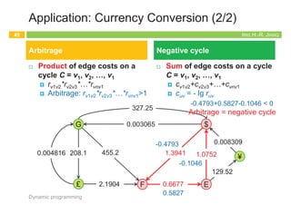
Application: Currency Conversion (1/2)
¨ Q: Given n currencies and exchange rates between pairs of
currencies, is there an arbitrage opportunity?
¤ The currency graph:
n Node: currency; edge cost: exchange rate ruv: ruv*rvu <1
¤ Arbitrage: a cycle on which product of edge costs >1
n E.g., $1 Þ 1.3941 Francs Þ 0.9308 Euros Þ $1.00084
Dynamic programming
48
Courtesy of Prof. Kevin Wayne @ Princeton
G
£ F E
¥
$
0.003065
455.2
208.1
0.004816
2.1904
1.3941
0.6677
327.25
129.52
0.008309
1.0752
$
1.3941
F 0.6677 E
1.0752](https://image.slidesharecdn.com/algorithm6dynamicprogramming-220522073057-711c84d9/85/algorithm_6dynamic_programming-pdf-45-320.jpg)
![IRIS H.-R. JIANG
Running Time
¨ Lines 5-6:
¤ Naïve: for each v, check v and others: O(n2)
¤ Detailed: for each v, check v and its neighbors (out-going edges):
åvÎV(degout(v)+1) = O(m)
¨ Lines 4-6:
¤ Naïve: O(n3)
¤ Detailed: O(nm)
Dynamic programming
45
0 1 2 3 4 5
n
t
b
c
d
a
e
n
¥
¥
¥
¥
¥
0
¥
3
4
-3
2
0
0
3
3
-3
0
0
-2
3
3
-4
0
0
-2
3
2
-6
0
0
-2
3
0
-6
0
0
b
d
t
e
-1
-2
4
2
c
-3
8
a
-4
6 -3
3
Bellman-Ford(G, s, t)
:
4. for i = 1 to n-1 do
5. for vÎV in any order do
6. M[i, v]=min{M[i-1, v], min(v, w)ÎE {cvw + M[i-1, w]}}
IRIS H.-R. JIANG
Space Improvement
¨ Maintain a 1D array instead:
¤ M[v] = shortest v-t path length that we have found so far.
¤ Iterator i is simply a counter
¤ No need to check edges of the form (v, w) unless M[w] changed
in previous iteration.
¤ In each iteration, for each node v,
M[v]=min{M[v], minwÎV {cvw + M[w]}}
¨ Observation: Throughout the algorithm, M[v] is the length of some
v-t path, and after i rounds of updates, the value M[v] is no larger
than the length of shortest v-t path using at most i edges.
Dynamic programming
46
Computing Science is –and will always be– concerned with the interplay
between mechanized and human symbol manipulation, which usually referred
to as “computing” and “programming” respectively.
~ E. W. Dijkstra
IRIS H.-R. JIANG
Negative Cycles?
¨ If a s-t path in a general graph G passes through node v, and v
belongs to a negative cycle C, Bellman-Ford algorithm fails to
find the shortest s-t path.
¤ Reduce cost over and over again using the negative cycle
Dynamic programming
47
v
s t
C c(C) < 0
IRIS H.-R. JIANG
Application: Currency Conversion (1/2)
¨ Q: Given n currencies and exchange rates between pairs of
currencies, is there an arbitrage opportunity?
¤ The currency graph:
n Node: currency; edge cost: exchange rate ruv: ruv*rvu <1
¤ Arbitrage: a cycle on which product of edge costs >1
n E.g., $1 Þ 1.3941 Francs Þ 0.9308 Euros Þ $1.00084
Dynamic programming
48
Courtesy of Prof. Kevin Wayne @ Princeton
G
£ F E
¥
$
0.003065
455.2
208.1
0.004816
2.1904
1.3941
0.6677
327.25
129.52
0.008309
1.0752
$
1.3941
F 0.6677 E
1.0752](https://image.slidesharecdn.com/algorithm6dynamicprogramming-220522073057-711c84d9/85/algorithm_6dynamic_programming-pdf-46-320.jpg)
![IRIS H.-R. JIANG
Running Time
¨ Lines 5-6:
¤ Naïve: for each v, check v and others: O(n2)
¤ Detailed: for each v, check v and its neighbors (out-going edges):
åvÎV(degout(v)+1) = O(m)
¨ Lines 4-6:
¤ Naïve: O(n3)
¤ Detailed: O(nm)
Dynamic programming
45
0 1 2 3 4 5
n
t
b
c
d
a
e
n
¥
¥
¥
¥
¥
0
¥
3
4
-3
2
0
0
3
3
-3
0
0
-2
3
3
-4
0
0
-2
3
2
-6
0
0
-2
3
0
-6
0
0
b
d
t
e
-1
-2
4
2
c
-3
8
a
-4
6 -3
3
Bellman-Ford(G, s, t)
:
4. for i = 1 to n-1 do
5. for vÎV in any order do
6. M[i, v]=min{M[i-1, v], min(v, w)ÎE {cvw + M[i-1, w]}}
IRIS H.-R. JIANG
Space Improvement
¨ Maintain a 1D array instead:
¤ M[v] = shortest v-t path length that we have found so far.
¤ Iterator i is simply a counter
¤ No need to check edges of the form (v, w) unless M[w] changed
in previous iteration.
¤ In each iteration, for each node v,
M[v]=min{M[v], minwÎV {cvw + M[w]}}
¨ Observation: Throughout the algorithm, M[v] is the length of some
v-t path, and after i rounds of updates, the value M[v] is no larger
than the length of shortest v-t path using at most i edges.
Dynamic programming
46
Computing Science is –and will always be– concerned with the interplay
between mechanized and human symbol manipulation, which usually referred
to as “computing” and “programming” respectively.
~ E. W. Dijkstra
IRIS H.-R. JIANG
Negative Cycles?
¨ If a s-t path in a general graph G passes through node v, and v
belongs to a negative cycle C, Bellman-Ford algorithm fails to
find the shortest s-t path.
¤ Reduce cost over and over again using the negative cycle
Dynamic programming
47
v
s t
C c(C) < 0
IRIS H.-R. JIANG
Application: Currency Conversion (1/2)
¨ Q: Given n currencies and exchange rates between pairs of
currencies, is there an arbitrage opportunity?
¤ The currency graph:
n Node: currency; edge cost: exchange rate ruv: ruv*rvu <1
¤ Arbitrage: a cycle on which product of edge costs >1
n E.g., $1 Þ 1.3941 Francs Þ 0.9308 Euros Þ $1.00084
Dynamic programming
48
Courtesy of Prof. Kevin Wayne @ Princeton
G
£ F E
¥
$
0.003065
455.2
208.1
0.004816
2.1904
1.3941
0.6677
327.25
129.52
0.008309
1.0752
$
1.3941
F 0.6677 E
1.0752](https://image.slidesharecdn.com/algorithm6dynamicprogramming-220522073057-711c84d9/85/algorithm_6dynamic_programming-pdf-47-320.jpg)
![IRIS H.-R. JIANG
Running Time
¨ Lines 5-6:
¤ Naïve: for each v, check v and others: O(n2)
¤ Detailed: for each v, check v and its neighbors (out-going edges):
åvÎV(degout(v)+1) = O(m)
¨ Lines 4-6:
¤ Naïve: O(n3)
¤ Detailed: O(nm)
Dynamic programming
45
0 1 2 3 4 5
n
t
b
c
d
a
e
n
¥
¥
¥
¥
¥
0
¥
3
4
-3
2
0
0
3
3
-3
0
0
-2
3
3
-4
0
0
-2
3
2
-6
0
0
-2
3
0
-6
0
0
b
d
t
e
-1
-2
4
2
c
-3
8
a
-4
6 -3
3
Bellman-Ford(G, s, t)
:
4. for i = 1 to n-1 do
5. for vÎV in any order do
6. M[i, v]=min{M[i-1, v], min(v, w)ÎE {cvw + M[i-1, w]}}
IRIS H.-R. JIANG
Space Improvement
¨ Maintain a 1D array instead:
¤ M[v] = shortest v-t path length that we have found so far.
¤ Iterator i is simply a counter
¤ No need to check edges of the form (v, w) unless M[w] changed
in previous iteration.
¤ In each iteration, for each node v,
M[v]=min{M[v], minwÎV {cvw + M[w]}}
¨ Observation: Throughout the algorithm, M[v] is the length of some
v-t path, and after i rounds of updates, the value M[v] is no larger
than the length of shortest v-t path using at most i edges.
Dynamic programming
46
Computing Science is –and will always be– concerned with the interplay
between mechanized and human symbol manipulation, which usually referred
to as “computing” and “programming” respectively.
~ E. W. Dijkstra
IRIS H.-R. JIANG
Negative Cycles?
¨ If a s-t path in a general graph G passes through node v, and v
belongs to a negative cycle C, Bellman-Ford algorithm fails to
find the shortest s-t path.
¤ Reduce cost over and over again using the negative cycle
Dynamic programming
47
v
s t
C c(C) < 0
IRIS H.-R. JIANG
Application: Currency Conversion (1/2)
¨ Q: Given n currencies and exchange rates between pairs of
currencies, is there an arbitrage opportunity?
¤ The currency graph:
n Node: currency; edge cost: exchange rate ruv: ruv*rvu <1
¤ Arbitrage: a cycle on which product of edge costs >1
n E.g., $1 Þ 1.3941 Francs Þ 0.9308 Euros Þ $1.00084
Dynamic programming
48
Courtesy of Prof. Kevin Wayne @ Princeton
G
£ F E
¥
$
0.003065
455.2
208.1
0.004816
2.1904
1.3941
0.6677
327.25
129.52
0.008309
1.0752
$
1.3941
F 0.6677 E
1.0752](https://image.slidesharecdn.com/algorithm6dynamicprogramming-220522073057-711c84d9/85/algorithm_6dynamic_programming-pdf-48-320.jpg)


The document outlines the principles of dynamic programming, emphasizing its application in optimization problems, including weighted interval scheduling, maze routing, and the traveling salesman problem. It discusses the methodology involving recursion and memoization to break down problems into manageable subproblems while also contrasting it with divide-and-conquer approaches. The document provides examples and emphasizes the importance of efficiently handling recursive calls to optimize performance.