This document is the preface to a book titled "1000 Solved Problems in Modern Physics" by Ahmad A. Kamal. It was published in 2010 by Springer-Verlag Berlin Heidelberg. The book contains solved problems in various topics in modern physics at the undergraduate level. It is divided into 10 chapters covering areas such as mathematical physics, quantum mechanics, thermodynamics, solid state physics, relativity, nuclear physics, and particle physics. The preface provides an overview of the content and structure of the book and acknowledges those who assisted in its preparation. It is intended to help physics students in solving assignments and preparing for exams.


![1.1 Basic Concepts and Formulae 15
Equivalence
A and B are said to be equivalent (A ∼ B) if one can be obtained from the other by
a sequence of elementary transformations.
The adjoint of a square matrix
If A = [ai j ] is a square matrix and αi j the cofactor of ai j then
adj A =
⎡
⎢
⎢
⎣
α11 α21 · · · αn1
α12 α22 · · · · · ·
· · · · · · · · · · · ·
· · · · · · · · · αnn
⎤
⎥
⎥
⎦
The cofactor αi j = (−1)i+ j
Mi j
where Mi j is the minor obtained by striking off the ith row and jth column and
computing the determinant from the remaining elements.
Inverse from the adjoint
A−1
=
adj A
|A|
Inverse for orthogonal matrices
A−1
= A
Inverse of unitary matrices
A−1
= (A)
Characteristic equation
Let AX = λX (1.84)
be the transformation of the vector X into λX, where λ is a number, then λ is called
the eigen or characteristic value.
From (1.84):
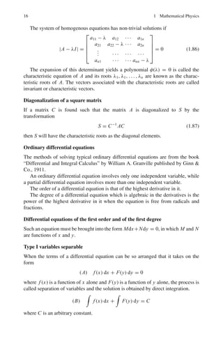
(A − λI)X =
⎡
⎢
⎢
⎢
⎣
a11 − λ a12 · · · a1n
a21 a22 − λ · · · a2n
.
.
. · · · · · · · · ·
an1 · · · · · · ann − λ
⎤
⎥
⎥
⎥
⎦
⎡
⎢
⎢
⎢
⎣
x1
x2
.
.
.
xn
⎤
⎥
⎥
⎥
⎦
= 0 (1.85)](https://image.slidesharecdn.com/1000-solved-problems-in-modern-physics-220626164600-18e7ea67/85/1000-solved-problems-in-modern-physics-pdf-35-320.jpg)
![26 1 Mathematical Physics
1.46 Show that:
4
2
2x + 4
x2 − 4x + 8
dx = ln 2 + π
1.47 Find the area included between the semi-cubical parabola y2
= x3
and the
line x = 4
1.48 Find the area of the surface of revolution generated by revolving the hypocy-
cloid x2/3
+ y2/3
= a2/3
about the x-axis.
1.49 Find the value of the definite double integral:
a
0
√
a2−x2
0
(x + y) dy dx
1.50 Calculate the area of the region enclosed between the curve y = 1/x, the
curve y = −1/x, and the lines x = 1 and x = 2.
1.51 Evaluate the integral:
dx
x2 − 18x + 34
1.52 Use integration by parts to evaluate:
1
0
x2
tan−1
x dx
[University of Wales, Aberystwyth 2006]
1.53 (a) Calculate the area bounded by the curves y = x2
+ 2 and y = x − 1 and
the lines x = −1 to the left and x = 2 to the right.
(b) Find the volume of the solid of revolution obtained by rotating the area
enclosed by the lines x = 0, y = 0, x = 2 and 2x + y = 5 through 2π
radians about the y-axis.
[University of Wales, Aberystwyth 2006]
1.54 Consider the curve y = x sin x on the interval 0 ≤ x ≤ 2π.
(a) Find the area enclosed by the curve and the x-axis.
(b) Find the volume generated when the curve rotates completely about the
x-axis.
1.2.8 Ordinary Differential Equations
1.55 Solve the differential equation:
dy
dx
=
x3
+ y3
3xy2](https://image.slidesharecdn.com/1000-solved-problems-in-modern-physics-220626164600-18e7ea67/85/1000-solved-problems-in-modern-physics-pdf-46-320.jpg)
![28 1 Mathematical Physics
1.63 Solve:
d2
y
dx2
− 8
dy
dx
= −16y
1.64 Solve:
x2 dy
dx
+ y(x + 1)x = 9x2
1.65 Find the general solution of the differential equation:
d2
y
dx2
+
dy
dx
− 2y = 2cosh(2x)
[University of Wales, Aberystwyth 2004]
1.66 Solve:
x
dy
dx
− y = x2
1.67 Find the general solution of the following differential equations and write
down the degree and order of the equation and whether it is homogenous or
in-homogenous.
(a) y
− 2
x
y = 1
x3
(b) y
+ 5y
+ 4y = 0
[University of Wales, Aberystwyth 2006]
1.68 Find the general solution of the following differential equations:
(a) dy
dx
+ y = e−x
(b) d2
y
dx2 + 4y = 2 cos(2x)
[University of Wales, Aberystwyth 2006]
1.69 Find the solution to the differential equation:
dy
dx
+
3
x + 2
y = x + 2
which satisfies y = 2 when x = −1, express your answer in the form y =
f (x).
1.70 (a) Find the solution to the differential equation:
d2
y
dx2
− 4
dy
dx
+ 4y = 8x2
− 4x − 4
which satisfies the conditions y = −2 and dy
dx
= 0 when x = 0.
(b) Find the general solution to the differential equation:
d2
y
dx2
+ 4y = sin x](https://image.slidesharecdn.com/1000-solved-problems-in-modern-physics-220626164600-18e7ea67/85/1000-solved-problems-in-modern-physics-pdf-48-320.jpg)
![30 1 Mathematical Physics
1.76 The Bessel function Jn (x) is given by the series expansion
Jn (x) =
(−1)k
(x/2)n+2k
k!Γ(n + k + 1)
Show that:
(a) d
dx
[xn
Jn(x) ] = xn
Jn−1(x)
(b) d
dx
[x−n
Jn(x)] = −x−n
Jn+1(x)
1.77 Prove the following relations for the Bessel functions:
(a) Jn−1(x) − Jn+1(x) = 2 d
dx
Jn(x)
(b) Jn−1(x) + Jn+1(x) = 2n
x
Jn(x)
1.78 Given that Γ
1
2
=
√
π, obtain the formulae:
(a) J1/2(x) =
$
2
πx
sin x
(b) J−1/2(x) =
$
2
πx
cos x
1.79 Show that the Legendre polynomials have the property:
l
−l
Pn(x)Pm(x) dx =
2
2n + 1
, if m = n
= 0, if m
= n
1.80 Show that for large n and small θ, Pn(cos θ) ≈ J0(nθ)
1.81 For Legendre polynomials Pl (x) the generating function is given by:
T (x, s) = (1 − 2sx + s2
)−1/2
=
∞
l=0
Pl(x)sl
, s 1
Use the generating function to show:
(a) (l + 1)Pl+1 = (2l + 1)x Pl − l Pl−1
(b) Pl(x) + 2x P
l (x) = P
l+1(x) + P
l−1(x), Where prime means differentiation
with respect to x.
1.82 For Laguerre’s polynomials, show that Ln(0) = n!. Assume the generating
function:
e−xs/(1−s)
1 − s
=
∞
n=0
Ln(x)sn
n!
1.2.11 Complex Variables
1.83 Evaluate
!
c
dz
z−2
where C is:
(a) The circle |z| = 1
(b) The circle |z + i| = 3](https://image.slidesharecdn.com/1000-solved-problems-in-modern-physics-220626164600-18e7ea67/85/1000-solved-problems-in-modern-physics-pdf-50-320.jpg)
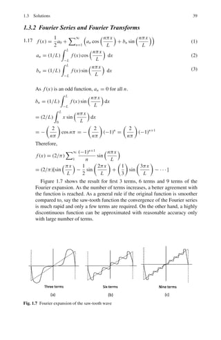
![32 1 Mathematical Physics
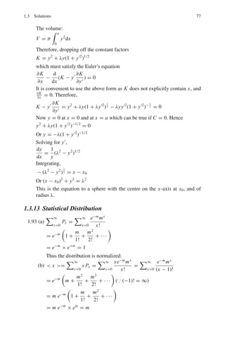
Fig. 1.5 Soap film stretched
between two parallel circular
wires
1.2.13 Statistical Distributions
1.93 Poisson distribution gives the probability that x events occur in unit time
when the mean rate of occurrence is m.
Px =
e−m
mx
x!
(a) Show that Px is normalized.
(b) Show that the mean rate of occurrence or the expectation value x , is
equal to m.
(c) Show that the S.D., σ =
√
m
(d) Show that Pm−1 = Pm
(e) Show that Px−1 = x
m
Pm and Px+1 = m
x+1
Px
1.94 The probability of obtaining x successes in N-independent trials of an event
for which p is the probability of success and q the probability of failure in a
single trial is given by the Binomial distribution:
B(x) =
N!
x!(N − x)!
px
qN−x
= CN
x px
qN−x
(a) Show that B(x) is normalized.
(b) Show that the mean value is Np
(c) Show that the S.D. is
√
Npq
1.95 A G.M. counter records 4,900 background counts in 100 min. With a radioac-
tive source in position, the same total number of counts are recorded in
20 min. Calculate the percentage of S.D. with net counts due to the source.
[Osmania University 1964]
1.96 (a) Show that when p is held fixed, the Binomial distribution tends to a nor-
mal distribution as N is increased to infinity.
(b) If Np is held fixed, then binomial distribution tends to Poisson distribu-
tion as N is increased to infinity.
1.97 The background counting rate is b and background plus source is g. If the
background is counted for the time tb and the background plus source for a
time tg, show that if the total counting time is fixed, then for minimum sta-
tistical error in the calculated counting rate of the source(s), tb and tg should
be chosen so that tb/tg =
√
b/g](https://image.slidesharecdn.com/1000-solved-problems-in-modern-physics-220626164600-18e7ea67/85/1000-solved-problems-in-modern-physics-pdf-52-320.jpg)
![1.3 Solutions 33
1.98 The alpha ray activity of a material is measured after equal successive inter-
vals (hours), in terms of its initial activity as unity to the 0.835; 0.695; 0.580;
0.485; 0.405 and 0.335. Assuming that the activity obeys an exponential
decay law, find the equation that best represents the activity and calculate
the decay constant and the half-life.
[Osmania University 1967]
1.99 Obtain the interval distribution and hence deduce the exponential law of
radioactivity.
1.100 In a Carbon-dating experiment background counting rate = 10 C/M. How
long should the observations be made in order to have an accuracy of 5%?
Assume that both the counting rates are measured for the same time.
14
C + background rate = 14.5 C/M
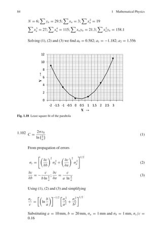
1.101 Make the best fit for the parabola y = a0 + a1x + a2x2
, with the given pairs
of values for x and y.
x −2 −1 0 +1 +2 +3
y 9.1 3.5 0.5 0.8 4.6 11.0
1.102 The capacitance per unit length of a capacitor consisting of two long concen-
tric cylinder with radii a and b, (b a) is C = 2πε0
ln(b/a)
. If a = 10 ± 1 mm and
b = 20 ± 1 mm, with what relative precision is C measured?
[University of Cambrdige Tripos 2004]
1.103 If f (x) is the probability density of x given by f (x) = xe−x/λ
over the
interval 0 x ∞, find the mean and the most probable values of x.
1.2.14 Numerical Integration
1.104 Calculate
10
1 x2
dx, by the trapezoidal rule.
1.105 Calculate
10
1 x2
dx, by the Simpson’s rule.
1.3 Solutions
1.3.1 Vector Calculus
1.1 ∇Φ =
î
∂
∂x
+ ĵ
∂
∂y
+ k̂
∂
∂z
(x2
+ y2
+ z2
)−1/2
=
−
1
2
.2xî −
1
2
.2y ĵ −
1
2
.2zk̂
(x2
+ y2
+ z2
)−3/2
= −(xî + y ĵ + zk̂)(x2
+ y2
+ z2
)− 3
2 = −
r
r3](https://image.slidesharecdn.com/1000-solved-problems-in-modern-physics-220626164600-18e7ea67/85/1000-solved-problems-in-modern-physics-pdf-53-320.jpg)
![34 1 Mathematical Physics
1.2 ∇(xy2
+ xz) =
î
∂
∂x
+ ĵ
∂
∂y
+ k̂
∂
∂z
(xy2
+ xz)
= (y2
+ z)î + (2xy) ĵ + xk̂
= 2î − 2 ĵ − k̂, at(−1, 1, 1)
A unit vector normal to the surface is obtained by dividing the above vector
by its magnitude. Hence the unit vector is
(2î − 2 ĵ − k̂)[(2)2
+ (−2)2
+ (−1)2
]−1/2
=
2
3
î −
2
3
ĵ −
1
3
k̂
1.3 F ∝ 1/r2
∇ . (r−3
r) = r−3
∇ . r + r . ∇r−3
But ∇ . r =
î
∂
∂x
+ ĵ
∂
∂y
+ k̂
∂
∂z
.
îx + ĵ y + k̂z
=
∂x
∂x
+
∂y
∂y
+
∂z
∂z
= 3
r . ∇r−3
= (xî + y ĵ + zk̂) .
î
∂
∂x
+ ĵ
∂
∂y
+ k̂
∂
∂z
(x2
+ y2
+ z2
)−3/2
= (xî + y ĵ + zk̂) .
−
3
2
. (2xî + 2y ĵ + 2zk̂)(x2
+ y2
+ z2
)−5/2
= −3(x2
+ y2
+ z2
)(x2
+ y2
+ z2
)− 5
2 = −3r−3
Thus ∇ . (r−3
r) = 3r−3
− 3r−3
= 0
1.4 By problem ∇ × A = 0 and ∇ × B = 0, it follows that
B . (∇ × A) = 0
A. (∇ × B) = 0
Subtracting, B . (∇ × A) − A . (∇ × B) = 0
Now ∇ . (A × B) = B . (∇ × A) − A . (∇ × B)
Therefore ∇ . (A × B) = 0, so that (A × B) is solenoidal.
1.5 (a) Curl {r f (r)} = ∇ × {r f (r)} = ∇ × {x f (r)î + y f (r) ĵ + zf (r)k̂}
=
%
%
%
%
%
%
%
%
î ĵ k̂
∂
∂x
∂
∂y
∂
∂z
x f (r) y f (r) zf (r)
%
%
%
%
%
%
%
%
=
z
∂ f
∂y
− y
∂ f
∂z
î +
x
∂ f
∂z
− z
∂ f
∂x
ĵ +
y
∂ f
∂x
− x
∂ f
∂y
k̂
But ∂ f
∂x
=
∂ f
∂r
∂r
∂x
= ∂ f
∂r
∂(x2
+y2
+z2
)1/2
∂x
= x f
r
Similarly ∂ f
∂y
= yf
r
and ∂ f
∂z
= zf
r
, where prime means differentiation with
respect to r.
Thus,
curl{r f (r)} =
zy f
r
−
yzf
r
î +
xzf
r
−
zx f
r
ĵ +
yx f
r
−
xy f
r
k̂ = 0](https://image.slidesharecdn.com/1000-solved-problems-in-modern-physics-220626164600-18e7ea67/85/1000-solved-problems-in-modern-physics-pdf-54-320.jpg)
![1.3 Solutions 35
(b) If the field is solenoidal, then, ∇.rF(r) = 0
∂(x F(r))
∂x
+
∂(yF(r))
∂y
+
∂(zF(r))
∂z
= 0
F + x
∂F
∂x
+ F + y
∂F
∂y
+ F + z
∂ F
∂z
= 0
3F(r) + x
∂F
∂r
x
r
+ y
∂ F
∂r
y
r
+ z
∂F
∂r
z
r
= 0
3F(r) +
∂ F
∂r
x2
+ y2
+ z2
r
= 0
But (x2
+ y2
+ z2
) = r2
, therefore, ∂F
∂r
= −3F(r)
r
Integrating, ln F = −3 lnr + ln C where C = constant
ln F = − lnr3
+ ln C = ln
C
r3
Therefore F = C/r3
. Thus, the field is A =
r
r3
(inverse square law)
1.6 x = t, y = t2
, z = t3
Therefore, y = x2
, z = x3
, dy = 2xdx, dz = 3x2
dx
c
A.dr =
(yî + xz ĵ + xyzk̂).(îdx + ĵdy + k̂dz)
=
1
0
x2
dx + 2
1
0
x5
dx + 3
1
0
x8
dx
=
1
3
+
1
3
+
1
3
= 1
1.7 The two curves y = x2
and y2
= 8x intersect at (0, 0) and (2, 4). Let us
traverse the closed curve in the clockwise direction, Fig. 1.6.
c
A.dr =
c
[(x + y)î + (x − y) ĵ].(î dx + ĵ dy)
=
c
[(x + y)dx + (x − y)dy]
=
0
2
[(x + x2
)dx + (x − x2
)2xdx] (along y = x2
)
Fig. 1.6 Line integral for a
closed curve](https://image.slidesharecdn.com/1000-solved-problems-in-modern-physics-220626164600-18e7ea67/85/1000-solved-problems-in-modern-physics-pdf-55-320.jpg)
![38 1 Mathematical Physics
A unit vector normal to the surface is obtained by dividing the above
vector by its magnitude. Hence the unit vector is
−î + ĵ + k̂
[(−1)2 + 12 + 12]1/2
= −
î
√
3
+
ĵ
√
3
+
k̂
√
3
(b) ∇Φ =
î
∂
∂x
+ ĵ
∂
∂y
+ k̂
∂
∂z
(x2
yz + 2xz2
)
= (2xyz + 2z2
)î + x2
z ĵ + 4xzk̂
= − ĵ − 4k̂ at (1, 1, −1)
The unit vector in the direction of 2î − 2 ĵ + k̂, is
n̂ =
2î − 2 ĵ + k̂
[22 + (−2)2 + 12]1/2
= 2î/3 − 2 ĵ/3 + k̂/3
The required directional derivative is
∇Φ.n = (− ĵ − 4k̂).
2î
3
−
2 ĵ
3
+
2k̂
3
#
=
2
3
−
4
3
= −
2
3
Since this is negative, it decreases in this direction.
1.15 The inverse square force can be written as
f α
r
r3
∇. f = ∇.r−3
r = r−3
∇. r + r .∇r−3
But ∇. r =
î
∂
∂x
+ ĵ
∂
∂y
+ k̂
∂
∂z
· (îx + ĵ y + k̂z)
=
∂x
∂x
+
∂y
∂y
+
∂z
∂z
= 3
Now ∇rn
= nrn−2
r
so that ∇r−3
= −3r−5
r
∴ ∇. (r−3
r) = 3r−3
− 3r−5
r . r = 3r−3
− r−3
= 0
Thus, the divergence of an inverse square force is zero.
1.16 The angle between the surfaces at the point is the angle between the normal to
the surfaces at the point.
The normal to x2
+ y2
+ z2
= 1 at (1, +1, −1) is
∇Φ1 = ∇(x2
+ y2
+ z2
) = 2xî + 2y ĵ + 2zk̂ = 2î + 2 ĵ − 2k̂
The normal to z = x2
+ y2
− 1 or x2
+ y2
− z = 1 at (1, 1, −1) is
∇Φ2 = ∇(x2
+ y2
− z) = 2xî + 2y ĵ − k̂ = 2î + 2 ĵ − k̂
(∇Φ1).(∇Φ2) = |∇Φ1||∇Φ2| cos θ
where θ is the required angle.
(2î + 2 ĵ − 2k̂).(2î + 2 ĵ − k̂) = (12)1/2
(9)1/2
cos θ
∴ cos θ =
10
6
√
3
= 0.9623
θ = 15.780](https://image.slidesharecdn.com/1000-solved-problems-in-modern-physics-220626164600-18e7ea67/85/1000-solved-problems-in-modern-physics-pdf-58-320.jpg)
![1.3 Solutions 39
1.3.2 Fourier Series and Fourier Transforms
1.17 f (x) =
1
2
a0 +
∞
n=1
an cos
nπx
L
+ bn sin
nπx
L
(1)
an = (1/L)
L
−L
f (x) cos
nπx
L
dx (2)
bn = (1/L)
L
−L
f (x) sin
nπx
L
dx (3)
As f (x) is an odd function, an = 0 for all n.
bn = (1/L)
L
−L
f (x) sin
nπx
L
dx
= (2/L)
L
0
x sin
nπx
L
dx
= −
2
nπ
cos nπ = −
2
nπ
(−1)n
=
2
nπ
(−1)n+1
Therefore,
f (x) = (2/π)
∞
1
(−1)n+1
n
sin
nπx
L
= (2/π)[sin
πx
L
−
1
2
sin
2πx
L
+
1
3
sin
3πx
L
− · · · ]
Figure 1.7 shows the result for first 3 terms, 6 terms and 9 terms of the
Fourier expansion. As the number of terms increases, a better agreement with
the function is reached. As a general rule if the original function is smoother
compared to, say the saw-tooth function the convergence of the Fourier series
is much rapid and only a few terms are required. On the other hand, a highly
discontinuous function can be approximated with reasonable accuracy only
with large number of terms.
Fig. 1.7 Fourier expansion of the saw-tooth wave](https://image.slidesharecdn.com/1000-solved-problems-in-modern-physics-220626164600-18e7ea67/85/1000-solved-problems-in-modern-physics-pdf-59-320.jpg)
![40 1 Mathematical Physics
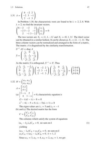
1.18 The given function is of the square form. As f (x) is defined in the interval
(−π, π), the Fourier expansion is given by
f (x) =
1
2
a0 +
∞
n=1
(an cos nx + bn sin nx) (1)
where an = (1/π)
π
−π
f (x) cos nx dx (2)
a0 = (1/π)
π
−π
f (x) dx (3)
bn =
1
π
π
−π
f (x) sin nx dx (4)
By (3)
a0 = (1/π)
0
−π
0dx +
π
0
πdx
= π (5)
By (2)
an = (1/π)
π
0
cos nx dx = 0, n ≥ 1 (6)
By (4)
bn = (1/π)
π
0
π sin nx dx =
1
n
(1 − cos nπ) (7)
Using (5), (6) and (7) in (1)
f (x) =
π
2
+ 2
sin(x) +
1
3
sin 3x +
1
5
sin 5x + · · ·
The graph of f (x) is shown in Fig. 1.8. It consists of the x-axis from −π to 0
and of the line AB from 0 to π. A simple discontinuity occurs at x = 0 at
which point the series reduces to π/2.
Now,
π/2 = 1/2[ f (0−) + f (0+)]
Fig. 1.8 Fourier expansion of
a square wave](https://image.slidesharecdn.com/1000-solved-problems-in-modern-physics-220626164600-18e7ea67/85/1000-solved-problems-in-modern-physics-pdf-60-320.jpg)
![42 1 Mathematical Physics
1.21 Consider the Fourier integral theorem
f (x) =
2
π
∞
0
cos ax da
∞
0
e−u
cos au du
Put f (x) = e−x
. Now the definite integral
∞
0
e−bu
cos(au) du =
b
b2 + a2
Here
∞
0
e−u
cos au du =
1
1 + a2
∴
2
π
∞
0
cos ax
1 + a2
dx = f (x) or
∞
0
cos ax
1 + a2
=
π
2
e−x
1.22 The Gaussian distribution is centered on t = 0 and has root mean square
deviation τ.
f̃ (ω) =
1
√
2π
∞
−∞
f (t)e−iωt
dt
=
1
√
2π
∞
−∞
1
τ
√
2π
e−t2
/2τ2
e−iωt
dt
=
1
√
2π
∞
−∞
1
τ
√
2π
e−[t2
+2τ2
iωt+(τ2
iω)2
−(τ2
iω)2
]/2τ2
dt
=
1
√
2π
e− τ2ω2
2
1
τ
√
2π
∞
−∞
e
−(t+iτ2ω2)2
2τ2
dt
The expression in the Curl bracket is equal to 1 as it is the integral for a
normalized Gaussian distribution.
∴ f̃ (ω) =
1
√
2π
e− τ2ω2
2
which is another Gaussian distribution centered on zero and with a root mean
square deviation 1/τ.
1.3.3 Gamma and Beta Functions
1.23 Γ(z + 1) = limT→∞
T
0 e−x
xz
dx
Integrating by parts
Γ(z + 1) = lim
T →∞
[−xz
e−x
|T
0 + z
T
0
e−x
xz−1
dx]
= z limT →∞
T
0
e−x
xz−1
dx = zΓ (z)
because T z
e−T
→ 0 as T → ∞
Also, since Γ(1) =
∞
0 e−x
dx = 1
If z is a positive integer n,
Γ(n + 1) = n!](https://image.slidesharecdn.com/1000-solved-problems-in-modern-physics-220626164600-18e7ea67/85/1000-solved-problems-in-modern-physics-pdf-63-320.jpg)
![50 1 Mathematical Physics
Differentiating, limn=∞
− 2n
2(n+1)
= ∞
∞
Differentiating again, limn=∞
−2
2
= −1(= L)
%
%
%
%
1
L
%
%
%
% =
%
%
%
%
1
−1
%
%
%
% = 1
The series (A) is
I. Absolutely convergent when |Lx| 1 or |x|
%
% 1
L
%
% i.e. −
%
% 1
L
%
% x
+
%
% 1
L
%
%
II. Divergent when |Lx| 1, or |x|
%
% 1
L
%
%
III. No test when |Lx| = 1, or |x| =
%
% 1
L
%
%.
By I the series is absolutely convergent when x lies between −1 and +1
By II the series is divergent when x is less than −1 or greater than +1
By III there is no test when x = ±1.
Thus the given series is said to have [−1, 1] as the interval of convergence.
1.36 f (x) = log x; f (1) = 0
f
(x) =
1
x
; f
(1) = 1
f
(x) = −
1
x2
; f
(1) = −1
f
(x) =
2
x3
; f
(1) = 2
Substitute in the Taylor series
f (x) = f (a) +
(x − a)
1!
f
(a) +
(x − a)2
2!
f
(a) +
(x − a)3
3!
f
(a) + · · ·
log x = 0 + (x − 1) −
1
2
(x − 1)2
+
1
3
(x − 1)2
− · · ·
1.37 Use the Maclaurin’s series
f (x) = f (0) +
x
1!
f
(0) +
x2
2!
f
(0) +
x3
3!
f
(0) + · · · (1)
Differentiating first and then placing x = 0, we get
f (x) = cos x, f (0) = 1
f
(x) = − sin x f
(0) = 0
f
(x) = − cos x, f
(0) = −1
f
(x) = sin x, f
(0) = 0
f iv
(x) = cos x, f iv
(0) = 1
etc.
Substituting in (1)
cos x = 1 −
x2
2!
+
x4
4!
−
x6
6!
+ · · ·
The series is convergent with all the values of x.](https://image.slidesharecdn.com/1000-solved-problems-in-modern-physics-220626164600-18e7ea67/85/1000-solved-problems-in-modern-physics-pdf-71-320.jpg)
![1.3 Solutions 53
1.45 (a)
tan6
x sec4
xdx =
tan6
x(tan2
x + 1) sec2
xdx
=
(tan x)8
sec2
xdx +
tan6
x sec2
xdx
=
(tan x)8
d(tan x) +
(tan x)6
d(tan x)
=
tan9
x
9
+
tan7
x
7
+ C
(b)
tan5
x sec3
xdx =
tan4
x sec2
x sec x tan x dx
=
(sec2
x − 1)2
sec2
x sec x tan x dx
=
(sec6
x − 2 sec4
x + sec2
x)d(sec x)
=
sec7
x
7
− 2
sec5
x
5
+
sec3
x
3
+ C
1.46
4
2
2x + 4
x2 − 4x + 8
dx =
4
2
2x − 4 + 8
(x − 2)2 + 4
dx
=
4
2
2x − 4
(x − 2)2 + 4
dx + 8
4
2
dx
(x − 2)2 + 4
= ln [(x − 2)2
+ 4]4
2 + (8/2) tan−1
1
= ln 2 + π
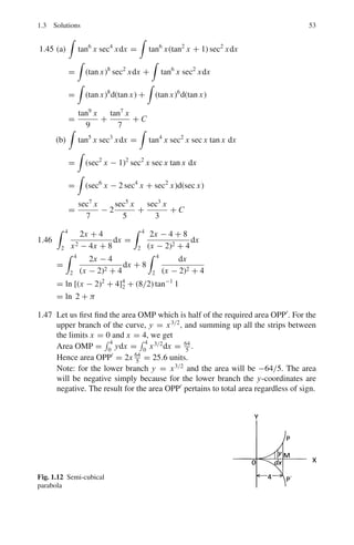
1.47 Let us first find the area OMP which is half of the required area OPP
. For the
upper branch of the curve, y = x3/2
, and summing up all the strips between
the limits x = 0 and x = 4, we get
Area OMP =
4
0 ydx =
4
0 x3/2
dx = 64
5
.
Hence area OPP
= 2x 64
5
= 25.6 units.
Note: for the lower branch y = x3/2
and the area will be −64/5. The area
will be negative simply because for the lower branch the y-coordinates are
negative. The result for the area OPP
pertains to total area regardless of sign.
Fig. 1.12 Semi-cubical
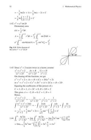
parabola](https://image.slidesharecdn.com/1000-solved-problems-in-modern-physics-220626164600-18e7ea67/85/1000-solved-problems-in-modern-physics-pdf-74-320.jpg)
![1.3 Solutions 59
The complete solution is
y = U + V (4)
where V = C3x + C4 (5)
In order that V be a particular solution of (1), substitute y = C3x + C4, in
(1) in order to determine C3 and C4.
−5C3 + 6(C3x + C4) = x
Equating the like coefficients
6C3 = 1 → C3 = 1/6
6C4 − 5C3 = 0 → C4 = 5/36
Hence the complete solution is
y = C1e2x
+ C2e3x
+
x
6
+
5
36
1.60
d2
x
dt2
+ 2
dx
dt
+ 5x = 0 (1)
Put x = eλt
, dx
dt
= λeλt
, d2
x
dt2 = λ2
eλt
in (1)
λ2
+ 2λ + 5 = 0 (2)
its roots being, λ = −1 ± 2i
x = Ae−t(1−2i)
+ Be−t(1+2i)
x = e−t
[C cos 2t + D sin 2t]
where C and D are constants to be determined from the initial conditions.
At t = 0, x = 5. Hence C = 5. Further
dx
dt
= −e−t
[C cos 2t + D sin 2t + 2C sin 2t − 2D cos 2t]
At t = 0, dx/dt = −3
−3 = −C + 2D = −5 + 2D
whence D = 1. Therefore the complete solution is
x = e−t
(5 cos 2t + sin 2t)
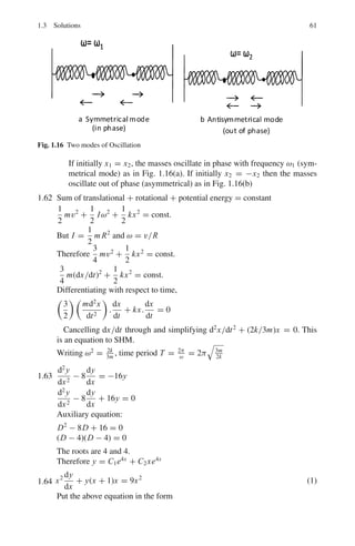
1.61 (a) Let the mass 1 be displaced by x1 and mass m2 by x2. The force due to the
spring on the left acting on mass 1 is −kx1 and that due to the coupling is
−k(x1 − x2).
The net force
F1 = −kx1 − k(x1 − x2) = −k(2x1 − x2)
The equation of motion for mass 1 is
mẍ1 + k(2x1 − x2) = 0 (1)
Similarly, for mass 2, the spring on the right exerts a force −kx2, and the
coupling spring exerts a force −k(x2 − x1). The net force
F2 = −kx2 − k(x2 − x1) = −k(2x2 − x1)](https://image.slidesharecdn.com/1000-solved-problems-in-modern-physics-220626164600-18e7ea67/85/1000-solved-problems-in-modern-physics-pdf-80-320.jpg)

![68 1 Mathematical Physics
=
λAλB N0
A
(λB − λA)
1
λA
1
s
−
1
s + λA
−
1
λB
1
s
−
1
s + λB
= N0
1
1
s
−
λB
(λB − λA)
1
(s + λA)
+
λA
(λB − λA)
1
(s + λB)
∴ Nc = N0
A
1 +
1
λB − λA
(λA exp (−λBt) − λB exp (−λAt))
1.74 (a) L{eax
} =
∞
0
e−sx
eax
dx =
∞
0
e−(s−a)x
dx
=
1
s − a
, if s a
(b) and (c). From part (a), L(eax
) = 1
s−a
Replace a by ai
L(eiax
) = L{cos ax + i sin ax}
= L{cos ax} + iL{sin ax}
=
1
s − ai
=
s + ai
s2 + a2
=
s
s2 + a2
+
ia
s2 + a2
Equating real and imaginary parts:
L{cos ax} =
s
s2 + a2
; L{sin ax} =
a
x2 + a2
1.3.10 Special Functions
1.75 Express Hn in terms of a generating function T (ξ, s).
T (ξ, s) = exp[ξ2
− (s − ξ)2
] = exp[−s2
+ 2sξ]
=
∞
n=0
Hn(ξ)sn
n!
(1)
Differentiate (1) first with respect to ξ and then with respect to s.
∂T
∂ξ
= 2s exp(−s2
+ 2sξ) =
n
2sn+1
Hn(ξ)
n!
=
n
sn
H
n(ξ)
n!
(2)
Equating equal powers of s
H
n = 2nHn−1 (3)
∂T
∂s
=ξ(−2s + 2ξ) exp(−s2
+2sξ)=
n
(−2s+2ξ)sn
Hn(ξ)=
n
sn−1
Hn(ξ)
(n − 1)!
(4)
Equating equal powers of s in the sums of equations
Hn+1 = 2ξ Hn − 2nHn−1 (5)
It is seen that (5) satisfies the Hermite’s equation](https://image.slidesharecdn.com/1000-solved-problems-in-modern-physics-220626164600-18e7ea67/85/1000-solved-problems-in-modern-physics-pdf-91-320.jpg)
![1.3 Solutions 69
H
n − 2ξ H
n + 2nHn = 0
1.76 Jn(x) =
k
(−1)k
x
2
n+2k
k!Γ (n + k + 1)
(a) Differentiate
d
dx
[xn
Jn(x)] = Jn(x)nxn−1
+ xn dJn(x)
dx
=
k
(−1)k
x
2
n+2k
nxn−1
k!Γ (n + k + 1)
+
xn
(n + 2k)(−1)k
xn+2k−1
k!Γ (n + k + 1).2n+2k
=
k
(−1)k
x
2
n+2k−1
(n + k)xn
k!Γ (n + k + 1)
=
(−1)k
x
2
n+2k−1
xn
Γ (n + k)
= xn
Jn−1(x)
(b) A similar procedure yields
d
dx
[x−n
Jn(x)] = −x−n
Jn+1(x)
1.77 From the result of 1.76(a)
d
dx
[xn
Jn(x)] = Jn(x)nxn−1
+ xn d Jn(x)
dx
= xn
Jn−1(x)
Divide through out by xn
n
x
Jn(x) +
dJn(x)
dx
= Jn−1(x)
Similarly from (b)
−
n
x
Jn(x) +
dJn(x)
dx
= −Jn+1(x)
Add and subtract to get the desired result.
1.78 Jn(x) =
∞
k=0
(−1)k
x
2
n+2k
k!Γ (n + k + 1)
(a) Therefore, with n = 1/2
J1
2
(x) =
x
2
1/2
Γ
3
2
−
x
2
5/2
1.Γ
5
2
+
x
2
9/2
2!Γ
7
2
− · · ·
Writing Γ
3
2
=
√
π
2
, Γ
5
2
= 3
√
π
4
, Γ
7
2
= 15
8
√
π
J1
2
(x) =](https://image.slidesharecdn.com/1000-solved-problems-in-modern-physics-220626164600-18e7ea67/85/1000-solved-problems-in-modern-physics-pdf-92-320.jpg)
![2
πx
cos x
1.79 The normalization of Legendre polynomials can be obtained by l – fold inte-
gration by parts for the conventional form
Pl(x) =
1
2ll!
dl
dxl
(x2
− 1)l
(Rodrigues’s formula)
+1
−1
[Pl(x)]2
dx =
1
2ll!
2 +1
−1
dl
(x2
− 1)l
dxl
dl
(x2
− 1)l
dxl
dx
= (−1)l
(
1
2ll!
)2
+1
−1
d2l
(x2
− 1)
dx2l
(x2
− 1)l
dx
= (−1)l
(2l)!
2ll!
2 +1
−1
(x2
− 1)l
dx =
2
2l + 1
Put l = n to get the desired result.
The orthogonality can be proved as follows. Legendre’s differential equation
d
dx
(1 − x2
)
dPn(x)
dx
+ n(n + 1)Pn(x) = 0 (1)
can be recast as
[(1 − x2
)P
n]
= −n(n + 1)Pn(x) (2)
[(1 − x2
)P
m]
= −m(m + 1)Pm(x) (3)
Multiply (2) by Pm and (3) by Pn and subtract the resulting expressions.
Pm[(1 − x2
)P
n]
− Pn[(1 − x2
)P
m]
= [m(m + 1) − n(n + 1)]Pm Pn (4)
Now, LHS of (4) can be written as
Pm[(1 − x2
)P
n]
− Pn[(1 − x2
)P
m]
= Pm[(1 − x2
)P
n]
+ P
m[(1 − x2
)P
n] − Pn[(1 − x2
)P
m] − Pn[(1 − x2
)P
m]
(4) can be integrated
d
dx
[(1 − x2
)(Pm P
n − Pn P
m) = [m(m + 1) − n(n + 1)]Pm Pn
(1 − x2
)
Pm P
n − Pn P
m
|1
−1 = [m(m + 1) − n(n + 1)]
1
−1
Pm Pndx
Since (1 − x2
) vanishes at x = ±1, the LHS is zero and the orthogonality
follows.
1
−1
Pm(x)Pn(x)dx = 0; m
= n](https://image.slidesharecdn.com/1000-solved-problems-in-modern-physics-220626164600-18e7ea67/85/1000-solved-problems-in-modern-physics-pdf-97-320.jpg)
![78 1 Mathematical Physics
(c) x2
=
x2 e−m
mx
x!
=
[x(x − 1) + x]
e−m
mx
x!
=
∞
x=0
e−m
mx
(x − 2)!
+
∞
x=0
x e−m mx
x!
= e−m
m2
+
m3
1!
+
m4
2!
+ · · ·
+ m
= m2
e−m
em
+ m = m2
+ m
σ2
= (x − x̄)2
= x2
−2 x x̄+ x̄ 2
= x2
−m2
σ2
= m or σ =
√
m
(d) Pm−1 =
e−m
mm−1
(m − 1)!
=
e−m
mm
(m − 1)!m
=
e−m
mm
m!
= Pm
That is the probability for the occurrence of the event at x = m − 1 is
equal to that at x = m
(e) Px−1 =
e−m
mx−1
(x − 1)!
=
e−m
mx
x!
x
m
=
x
m
Px
Px+1 =
e−m
mx+1
(x + 1)!
=
m e−m
mx
x!(x + 1)
=
m
x + 1
Px
1.94 (a) (q + p)N
= qN
+ NqN−1
P +
N(N − 1)qN−2
2!
P2
+ · · ·
N!
x!(N − x)!
Px
qN−x
+ · · · PN
=
N
x=0
N!
x!(N − x)!
Px
qN−x
= 1(∵ q + p = 1)
(b) We can use the moment generating function Mx (t) about the mean μ
which is given as
Mx (t) = Ee(x−μ)t
= E
1 + (x − μ)t + (x − μ)2 t2
2!
+ · · ·
= 1 + 0 + μ2
t2
2!
+ μ3
t3
3!
+ · · ·
So that μn is the coefficient of tn
n!](https://image.slidesharecdn.com/1000-solved-problems-in-modern-physics-220626164600-18e7ea67/85/1000-solved-problems-in-modern-physics-pdf-106-320.jpg)
![1.3 Solutions 79
Mx (t) = Eext
=
∞
x=0
ext
B(x)
=
∞
x=0
N
r
(pet
)r
(1 − p)N−r
= (pet
+ 1 − p)N
N
r
pr
qN−r
= (pet
+ 1 − p)N
μ0
n =
∂n
Mx (t)
∂tn
|t=0
Therefore μ0
1 = ∂M
∂t
|t=0 = Npet
(q + pet
)N−1
|t=0 = Np
Thus the mean = Np
(c) μ0
2 =
∂2
M
∂t2
= [N(N − 1)p2
et
(q + pet
)N−2
+ Npet
(q + pet
)N−1
]t=0
= N(N − 1)p2
+ Np
But μ2 = μ0
2 − (μ0
1)2
= N(N − 1)p2
+ Np − N2
p2
= Np − Np2
= Np(1 − p) = Npq
or σ =
Npq
1.95 Total counting rate/minute, m1 = 245
Background rate/minute, m2 = 49
Counting rate of source, m = m1 − m2 = 196
m1 =
n1
t1
±
√
n1
t1
; m2 =
n2
t2
±
√
n2
t2
; Net count m = m1 − m2
σ = (σ2
1 + σ2
2 )1/2
=
n1
t2
1
+
n2
t2
2
1/2
=
m1
t1
+
m2
t2
1/2
σ =
m1
t1
+
m2
t2
1/2
=
49
100
+
245
20
1/2
= 3.57
Percentage S.D. = σ
m
× 100 = 3.57
196
× 100 = 1.8%
1.96 (a) B(x) =
N!
x!(N − x)!
px
qN−x
Using Sterling’s theorem](https://image.slidesharecdn.com/1000-solved-problems-in-modern-physics-220626164600-18e7ea67/85/1000-solved-problems-in-modern-physics-pdf-107-320.jpg)
![92 2 Quantum Mechanics – I
2.2 Problems
2.2.1 de Broglie Waves
2.1 (a) Write down the equation relating the energy E of a photon to its frequency
f . Hence determine the equation relating the energy E of a photon to its
wavelength.
(b) A π0
meson at rest decays into two photons of equal energy. What is the
wavelength (in m) of the photons? (The mass of the π0
is 135 MeV/c)
[University of London 2006]
2.2 Calculate the wavelength in nm of electrons which have been accelerated from
rest through a potential difference of 54 V.
[University of London 2006]
2.3 Show that the deBroglie wavelength for neutrons is given by λ = 0.286 Å/
√
E,
where E is in electron-volts.
[Adapted from the University of New Castle upon Tyne 1966]
2.4 Show that if an electron is accelerated through V volts then the deBroglie wave-
length in angstroms is given by λ =
150
V
1/2
2.5 A thermal neutron has a speed v at temperature T = 300 K and kinetic energy
mnv2
2
= 3kT
2
. Calculate its deBroglie wavelength. State whether a beam of these
neutrons could be diffracted by a crystal, and why?
(b) Use Heisenberg’s Uncertainty principle to estimate the kinetic energy (in
MeV) of a nucleon bound within a nucleus of radius 10−15
m.
2.6 The relation for total energy (E) and momentum (p) for a relativistic particle
is E2
= c2
p2
+ m2
c4
, where m is the rest mass and c is the velocity of light.
Using the relativistic relations E = ω and p = k, where ω is the angular
frequency and k is the wave number, show that the product of group velocity
(vg) and the phase velocity (vp) is equal to c2
, that is vpvg = c2
2.2.2 Hydrogen Atom
2.7 In the Bohr model of the hydrogen-like atom of atomic number Z the atomic
energy levels of a single-electron are quantized with values given by
En =
Z2
mee4
8ε2
0h2n2
where m is the mass of the electron, e is the electronic charge and n is an
integer greater than zero (principal quantum number)](https://image.slidesharecdn.com/1000-solved-problems-in-modern-physics-220626164600-18e7ea67/85/1000-solved-problems-in-modern-physics-pdf-123-320.jpg)
![2.2 Problems 93
What additional quantum numbers are needed to specify fully an atomic quan-
tum state and what physical quantities do they quantify? List the allowed quan-
tum numbers for n = 1 and n = 2 and specify fully the electronic quantum
numbers for the ground state of the Carbon atom (atomic number Z = 6)
[Adapted from University of London 2002]
2.8 Estimate the total ground state energy in eV of the system obtained if all the
electrons in the Carbon atom were replaced by π−
particles. (You are given
that the ground state energy of the hydrogen atom is −13.6 eV and that the π−
is a particle with charge −1, spin 0 and mass 270 me
[University of London]
2.9 What are atomic units? In this system what are the units of (a) length (b) energy
(c) 2
(d) e2
(e) me ? (f) Write down Schrodinger’s equation for H-atom in
atomic units
2.10 (a) Two positive nuclei each having a charge q approach each other and elec-
trons concentrate between the nuclei to create a bond. Assume that the
electrons can be represented by a single point charge at the mid-point
between the nuclei. Calculate the magnitude this charge must have to
ensure that the potential energy is negative.
(b) A positive ion of kinetic energy 1 × 10⁻¹⁹
J collides with a stationary
molecule of the same mass and forms a single excited composite molecule.
Assuming the initial internal energies of the ion and neutral molecule were
zero, calculate the internal energy of the molecule.
[Adapted from University of Wales, Aberystwyth 2008]
2.11 (a) By using the deBroglie relation, derive the Bohr condition mvr = n for
the angular momentum of an electron in a hydrogen atom.
(b) Use this expression to show that the allowed electron energy states in
hydrogen atom can be written
En = −
me4
8ε2
0h2n2
(c) How would this expression be modified for the case of a triply ionized
beryllium atom Be(Z = 4)?
(d) Calculate the ionization energy in eV of Be+3
(ionization energy of hydro-
gen = 13.6 eV)
[Adapted from the University of Wales, Aberystwyth 2007]
2.12 When a negatively charged muon (mass 207 me is captured in a Bohr’s orbit
of high principal quantum number (n) to form a mesic atom, it cascades
down to lower orbits emitting X-rays and the radii of the mesic atom are
shrunk by a factor of about 200 compared with the corresponding Bohr’s atom.
Explain.
2.13 In which mu-mesic atom would the orbit with n = 1 just touch the nuclear
surface. Take Z = A/2 and R = 1.3 A1/3
fm.](https://image.slidesharecdn.com/1000-solved-problems-in-modern-physics-220626164600-18e7ea67/85/1000-solved-problems-in-modern-physics-pdf-124-320.jpg)
![94 2 Quantum Mechanics – I
2.14 Calculate the wavelengths of the first four lines of the Lyman series of the
positronium on the basis of the simple Bohr’s theory
[Saha Institute of Nuclear physics 1964]
2.15 (a) Show that the energy En of positronium is given by En = −α2
mec2
/4n2
where me is the electron mass, n the principal quantum number and α the
fine structure constant
(b) the radii are expanded to double the corresponding radii of hydrogen atom
(c) the transition energies are halved compared to that of hydrogen atom.
2.16 A non-relativistic particle of mass m is held in a circular orbit around the
origin by an attractive force f (r) = −kr where k is a positive constant
(a) Show that the potential energy can be written
U(r) = kr2
/2
Assuming U(r) = 0 when r = 0
(b) Assuming the Bohr quantization of the angular momentum of the particle,
show that the radius r of the orbit of the particle and speed v of the particle
can be written
v2
=
n
m
k
m
1/2
r2
=
n
k
k
m
1/2
where n is an integer
(c) Hence, show that the total energy of the particle is
En = n
k
m
1/2
(d) If m = 3 × 10⁻²⁶
kg and k = 1180 N m−1
, determine the wavelength of
the photon in nm which will cause a transition between successive energy
levels.
2.17 For high principle quantum number (n) for hydrogen atom show that the spac-
ing between the neighboring energy levels is proportional to 1/n3
.
2.18 In which transition of hydrogen atom is the wavelength of 486.1 nm produced?
To which series does it belong?
2.19 Show that for large quantum number n, the mechanical orbital frequency
is equal to the frequency of the photon which is emitted between adjacent
levels.
2.20 A hydrogen-like ion has the wavelength difference between the first lines of
the Balmer and lyman series equal to 16.58 nm. What ion is it?](https://image.slidesharecdn.com/1000-solved-problems-in-modern-physics-220626164600-18e7ea67/85/1000-solved-problems-in-modern-physics-pdf-125-320.jpg)
![2.2 Problems 95
2.21 A spectral line of atomic hydrogen has its wave number equal to the difference
between the two lines of Balmer series, 486.1 nm and 410.2 nm. To which
series does the spectral line belong?
2.2.3 X-rays
2.22 (a) The L → K transition of an X-ray tube containing a molybdenum (Z = 42)
target occurs at a wavelength of 0.0724 nm. Use this information to estimate
the screening parameter of the K-shell electrons in molybdenum.
[Osmania University]
2.23 Calculate the wavelength of the Mo(Z = 42)Kα X-ray line given that the
ionization energy of hydrogen is 13.6 eV
[Adapted from the University of London, Royal Holloway 2002]
2.24 In a block of Cobalt/iron alloy, it is suspected that the Cobalt (Z = 27) is
very poorly mixed with the iron (Z = 26). Given that the ionization energy
of hydrogen is 13.6 eV predict the energies of the K absorption edges of the
constituents of the alloy.
[University of London, Royal Holloway 2002]
2.25 Calculate the minimum wavelength of the radiation emitted by an X-ray tube
operated at 30 kV.
[Adapted from the University of London, Royal Holloway 2005]
2.26 If the minimum wavelength from an 80 kV X-ray tube is 0.15 × 10⁻¹⁰
m,
deduce a value for Planck’s constant.
[Adapted from the University of New Castle upon Tyne 1964]
2.27 If the minimum wavelength recorded in the continuous X-ray spectrum from
a 50 kV tube is 0.247 Å, calculate the value of Plank’s constant.
[Adapted from the University of Durham 1963]
2.28 The wavelength of the Kα line in iron (Z = 26) is known to be 193 pm. Then
what would be the wavelength of the Kα line in copper (Z = 29)?
2.29 An X-ray tube has nickel as target. If the wavelength difference between the
Kα line and the short wave cut-off wavelength of the continuous X-ray spec-
trum is equal to 84 pm, what is the voltage applied to the tube?
2.30 Consider the transitions in heavy atoms which give rise to Lα line in X-ray
spectra. How many allowed transitions are possible under the selection rule
Δl = ±1, Δ j = 0, ±1.
2.31 When the voltage applied to an X-ray tube increases from 10 to 20 kV the
wavelength difference between the Kα line and the short wave cut-off of the
continous X-ray spectrum increases by a factor of 3.0. Identify the target mate-
rial.
2.32 How many elements have the Kα lines between 241 and 180 pm?](https://image.slidesharecdn.com/1000-solved-problems-in-modern-physics-220626164600-18e7ea67/85/1000-solved-problems-in-modern-physics-pdf-126-320.jpg)
![96 2 Quantum Mechanics – I
2.33 Moseley’s law for characteristic x-rays is of the form
√
v = a(z−b). Calculate
the value of a for Kα
2.34 The Kα line has a wavelength λ for an element with atomic number Z = 19.
What is the atomic number of an element which has a wavelength λ/4 for the
Kα line?
2.2.4 Spin and μ and Quantum Numbers – Stern–Gerlah’s
Experiment
2.35 Evidence for the electron spin was provided by the Sterrn–Gerlah experiment.
Sketch and briefly describe the key features of the experiment. Explain what
was observed and how this observation may be interpreted in terms of electron
spin.
[Adapted from University of London 2006]
2.36 (i) Write down the allowed values of the total angular momentum quantum
number j, for an atom with spin s and l, respectively (ii) Write down the
quantum numbers for the states described as 2
S1/2, 3
D2 and 5
P3 (iii) Determine
if any of these states are impossible, and if so explain why.
[Adapted from the University of London, Royal Holloway 2003]
2.37 (a) show that an electron in a classical circular orbit of angular momentum
L around a nucleus has magnetic dipole moment given by μ = −e L/2me
(b) State the quantum mechanical values for the magnitude and the z-compo-
nent of the magnetic moment of the hydrogen atom associated with (i) electron
orbital angular momentum (ii) electron spin
[Adapted from the University of London, Royal Holloway 2004]
2.38 In a Stern-Gerlach experiment a collimated beam of hydrogen atoms emitted
from an oven at a temperature of 600 K, passes between the poles of a magnet
for a distance of 0.6 m before being detected at a photographic plate a further
1.0 m away. Derive the expression for the observed mean beam separation, and
determine its value given that the magnetic field gradient is 20 Tm−1
(Assume
the atoms to be in the ground state and their mean kinetic energy to be 2 kT;
Bohr magneton μB = 9.27 × 10⁻²⁴
J T−1
[Adapted from the University of London, Royal Holloway 2004]
2.39 State the ground state electron configuration and magnetic dipole moment of
hydrogen (Z = 1) and sodium (Z = 11)
2.40 In a Stern–Gerlah experiment a collimated beam of sodium atoms, emit-
ted from an oven at a temperature of 400 K, passes between the poles of
a magnet for a distance of 1.00 m before being detected on a screen a fur-
ther 0.5 m away. The mean deflection detected was 0.14◦
. Assuming that
the magnetic field gradient was 6.0 T m−1
and that the atoms were in the](https://image.slidesharecdn.com/1000-solved-problems-in-modern-physics-220626164600-18e7ea67/85/1000-solved-problems-in-modern-physics-pdf-127-320.jpg)
![2.2 Problems 97
ground state and their mean kinetic energy was 2kT, estimate the magnetic
moment.
[Adapted from the University of London, Royal Holloway and Bedford New
College, 2005]
2.41 If the electronic structure of an element is 1s2
2s2
2p6
3s2
3p6
3d10
4s2
4p5
,
why can it not be (a) a transition element (b) a rare-earth element?
[Adopted from the University of Manchester 1958]
2.42 In a Stern–Gerlach experiment the magnetic field gradient is 5.0 V s m−2
mm−1
,
with pole pieces 7 cm long. A narrow beam of silver atoms from an oven at
1, 250 K passes through the magnetic field. Calculate the separation of the
beams as they emerge from the magnetic field, pointing out the assumptions
you have made (Take μ = 9.27 × 10⁻²⁴
JT−1
]
[Adapted from the University of Durham 1962]
2.43 (a) The magnetic moment of silver atom is only 1 Bohr magneton although it
has 47 electrons? Explain.
(b) Ignoring the nuclear effects, what is the magnetic moment of an atom in
the 3p0 state?
(c) In a Stern–Gerlah experiment, a collimated beam of neutral atoms is split
up into 7 equally spaced lines. What is the total angular momentum of the
atom?
(d) what is the ratio of intensities of spectral lines in hydrogen spectrum for
the transitions
22
p1/2 → 12
s1/2 and 22
p3/2 → 12
s1/2?
2.44 Obtain an expression for the Bohr magneton.
2.2.5 Spectroscopy
2.45 (a) Given the allowed values of the quantum numbers n,l, m and ms of an
electron in a hydrogen atom (b) What are the allowed numerical values of
l and m for the n = 3 level? (c) Hence show that this level can accept 18
electrons.
[Adopted from University of London 2006]
2.46 State, with reasons, which of the following transitions are forbidden for elec-
tric dipole transitions
3
D1 → 2
F3
2
P3/2 → 2
S1/2
2
P1/2 → 2
S1/2
3
D2 → 3
S1](https://image.slidesharecdn.com/1000-solved-problems-in-modern-physics-220626164600-18e7ea67/85/1000-solved-problems-in-modern-physics-pdf-128-320.jpg)
![98 2 Quantum Mechanics – I
2.47 The 9
Be+
ion has a nucleus with spin I = 3/2. What values are possible for
the hyperfine quantum number F for the 2
S1/2 electronic level?
[Aligarh University]
2.48 Obtain an expression for the Doppler linewidth for a spectral line of wave-
length λ emitted by an atom of mass m at a temperature T
2.49 For the 2P3/2 → 2S1/2 transition of an alkali atom, sketch the splitting of the
energy levels and the resulting Zeeman spectrum for atoms in a weak exter-
nal magnetic field (Express your results in terms of the frequency v0 of the
transition, in the absence of an applied magnetic field)
The Lande g-factor is given by g = 1 +
j( j + 1) + s(s + 1) − l(l + 1)
2 j( j + 1)
[Adapted from the University of London Holloway 2002]
2.50 The spacings of adjacent energy levels of increasing energy in a calcium triplet
are 30 × 10−4
and 60 × 10−4
eV. What are the quantum numbers of the three
levels? Write down the levels using the appropriate spectroscopic notation.
[Adapted from the University of London, Royal Holloway 2003]
2.51 An atomic transition line with wavelength 350 nm is observed to be split into
three components, in a spectrum of light from a sun spot. Adjacent compo-
nents are separated by 1.7 pm. Determine the strength of the magnetic field in
the sun spot. μB = 9.17 × 10⁻²⁴
J T−1
[Adapted from the University of London, Royal Holloway 2003]
2.52 Calculate the energy spacing between the components of the ground state
energy level of hydrogen when split by a magnetic field of 1.0 T. What fre-
quency of electromagnetic radiation could cause a transition between these
levels? What is the specific name given to this effect.
[Adapted from the University of London, Royal Holloway 2003]
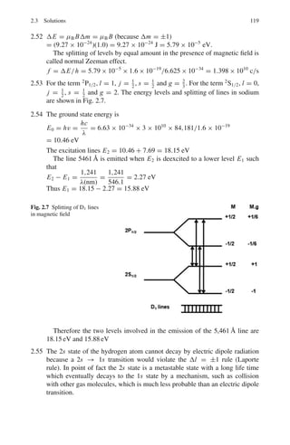
2.53 Consider the transition 2P1/2 → 2S1/2, for sodium in the magnetic field of
1.0 T, given that the energy splitting ΔE = gμB Bm j , where μB is the Bohr
magneton. Draw the sketch.
[Adapted from the University of London, Royal Holloway 2004]
2.54 To excite the mercury line 5,461 Å an excitation potential of 7.69 V is required.
If the deepest term in the mercury spectrum lies at 84,181 cm−1
, calculate the
numerical values of the two energy levels involved in the emission of 5,461 Å.
[The University of Durham 1963]
2.55 The mean time for a spontaneous 2p → 1s transition is 1.6 × 10⁻⁹
s while
the mean time for a spontaneous 2s → 1s transition is as long as 0.14 s.
Explain.](https://image.slidesharecdn.com/1000-solved-problems-in-modern-physics-220626164600-18e7ea67/85/1000-solved-problems-in-modern-physics-pdf-129-320.jpg)
![2.2 Problems 99
2.56 In the Helium-Neon laser (three-level laser), the energy spacing between the
upper and lower levels E2 − E1 = 2.26 in the neon atom. If the optical pump-
ing operation stops, at what temperature would the ratio of the population of
upper level E2 and the lower level E1, be 1/10?
2.2.6 Molecules
2.57 What are the two modes of motion of a diatomic molecule about its centre of
mass? Explain briefly the origin of the discrete energy level spectrum associ-
ated with one of these modes.
[University of London 2003]
2.58 Rotational spectral lines are examined in the HD (hydrogen–deuterium)
molecule. If the internuclear distance is 0.075 nm, estimate the wavelength
of radiation arising from the lowest levels.
2.59 Historically, the study of alternate intensities of spectral lines in the rotational
spectra of homonuclear molecules such as N2 was crucial in deciding the
correct model for the atom (neutrons and protons constituting the nucleus
surrounded by electrons outside, rather than the proton–electron hypothesis
for the Thomas model). Explain.
2.60 The force constant for the carbon monoxide molecule is 1,908 N m−1
. At
1,000 K what is the probability that the molecule will be found in the lowest
excited state?
2.61 At a given temperature the rotational states of molecules are distributed
according to the Boltzmann distribution. Of the hydrogen molecules in the
ground state estimate the ratio of the number in the ground rotational state to
the number in the first excited rotational state at 300 K. Take the interatomic
distance as 1.06 Å.
2.62 Estimate the wavelength of radiation emitted from adjacent vibration energy
levels of NO molecule. Assume the force constant k = 1,550 N m−1
. In which
region of electromagnetic spectrum does the radiation fall?
2.63 Carbon monoxide (CO) absorbs energy at 1.153×1,011 Hz, due to a transition
between the l = 0 and l = 1 rotational states.
(i) What is the corresponding wavelength? In which part of the electro-
magnetic spectrum does this lie?
(ii) What is the energy (in eV)?
(iii) Calculate the reduced mass μ. (C = 12 times, and O = 16 times the
unified atomic mass constant.)
(iv) Given that the rotational energy E = l(l+1)2
2μr2 , find the interatomic distance
r for this molecule.
2.64 Consider the hydrogen molecule H2 as a rigid rotor with distance of separation
of H-atoms r = 1.0 Å. Compute the energy of J = 2 rotational level.](https://image.slidesharecdn.com/1000-solved-problems-in-modern-physics-220626164600-18e7ea67/85/1000-solved-problems-in-modern-physics-pdf-130-320.jpg)
![100 2 Quantum Mechanics – I
2.65 The J = 0 → J = 1 rotational absorption line occurs at wavelength 0.0026
in C12
O16
and at 0.00272 m in Cx
O16
. Find the mass number of the unknown
Carbon isotope.
2.66 Assuming that the H2
molecule behaves like a harmonic oscillator with force
constant of 573 N/m. Calculate the vibrational quantum number for which the
molecule would dissociate at 4.5 eV.
2.2.7 Commutators
2.67 (a) Show that eipα/
x e−ipα/
= x + α
(b) If A and B are Hermitian, find the condition that the product AB will be
Hermitian
2.68 (a) If A is Hermitian, show that ei A
is unitary
(b) What operator may be used to distinguish between
(a) eikx
and e−ikx
(b) sin ax and cos ax?
2.69 (a) Show that exp (iσ xθ) = cos θ + iσ x sin θ
(b) Show that
d
dx
†
= − d
dx
2.70 Show that
(a) [x, px ] = [y, py] = [z, pz] = i
(b) [x2
, px ] = 2ix
2.71 Show that a hermitian operator is always linear.
2.72 Show that the momentum operator is hermitian
2.73 The operators P and Q commute and they are represented by the matrices
1 2
2 1
and
3 2
2 3
. Find the eigen vectors of P and Q. What do you notice
about these eigen vectors, which verify a necessary condition for commuting
operators?
2.74 An operator  is defined as  = αx̂ + iβ p̂, where α , β are real numbers
(a) Find the Hermitian adjoint operator †
(b) Calculate the commutators [Â, x̂], [Â, Â] and [Â, P̂]
2.75 A real operator A satisfies the lowest order equation.
A2
− 4A + 3 = 0
(a) Find the eigen values of A (b) Find the eigen states of A (c) Show that A
is an observable.
2.76 Show that (a) [x, H] = ip
μ
(b) [[x, H], x] = 2
μ
where H is the Hamiltonian.
2.77 Show that for any two operators A and B,
[A2
, B] = A[A, B] + [A, B]A](https://image.slidesharecdn.com/1000-solved-problems-in-modern-physics-220626164600-18e7ea67/85/1000-solved-problems-in-modern-physics-pdf-131-320.jpg)
![2.3 Solutions 101
2.78 Show that (σ.A)(σ.B) = A.B+iσ.(A×B) where A and B are vectors and σ’s
are Pauli matrices.
2.79 The Pauli matrix σy =
0 −i
i 0
(a) Show that the matrix is real whose eigen values are real.
(b) Find the eigen values of σy and construct the eigen vectors.
(c) Form the projector operators P1 and P2 and show that
P
†
1 P2 =
0 0
0 0
, P1 P
†
1 + P2 P
†
2 = I
2.80 The Pauli spin matrices are σx =
0 1
1 0
, σy =
0 −i
i 0
, σz =
1 0
0 −1
Show that (i) σ2
x = 1 and (ii) the commutator [σx , σy] = 2iσz.
2.81 The condition that must be satisfied by two operators  and B̂ if they are to
share the same eigen states is that they should commute. Prove the statement.
2.2.8 Uncertainty Principle
2.82 Use the uncertainty principle to obtain the ground state energy of a linear
oscillator
2.83 Is it possible to measure the energy and the momentum of a particle simulta-
neously with arbitrary precision?
2.84 Obtain Heisenberg’s restricted uncertainty relation for the position and momen-
tum.
2.85 Use the uncertainty principle to make an order of magnitude estimate for the
kinetic energy (in eV) of an electron in a hydrogen atom.
[University of London 2003]
2.86 Write down the two Heisenberg uncertainty relations, one involving energy
and one involving momentum. Explain the meaning of each term. Estimate
the kinetic energy (in MeV) of a neutron confined to a nucleus of diameter
10 fm.
[University of London 2006]
2.3 Solutions
2.3.1 de Broglie Waves
2.1 (a) E = h f = hλ/c
(b) Each photon carries an energy
Eγ =
mπ c2
2
=
135
2
= 67.5 MeV](https://image.slidesharecdn.com/1000-solved-problems-in-modern-physics-220626164600-18e7ea67/85/1000-solved-problems-in-modern-physics-pdf-132-320.jpg)
![102 2 Quantum Mechanics – I
cPγ = Eγ = 67.5 MeV
λ =
h
p
= 2π
c
cp
=
(2π)(197.3 MeV.fm)
67.5 MeV
= 18.36 fm = 1.836 × 10⁻¹⁴
m.
2.2 λ =
150
V
1/2
=
150
54
1/2
= 1.667 Å
2.3 λ =
h
p
=
2πc
(2mc2T )1/2
= (2π) ×
197.3 MeV − fm
(2 × 939 T − MeV)1/2
= 28.6 × 10⁻⁵
Å/T 1/2
where T is in MeV. If T is in eV, λ = 0.286 Å/T1/2
2.4 λ =
h
p
=
6.63 × 10⁻³⁴
J−s
(2 × 9.1 × 10−31 × 1.6 × 10−19)1/2
= 12.286 × 10⁻¹⁰
m/V1/2
=
151
V
1/2
.
2.5 (a)
mnv2
2
=
p2
2mn
=
3kT
2
=
3
2
× 1.38 × 10−23
×
300
1.6 × 10−19
= 0.0388 eV
cCp =
√
2mnc2
· En
1/2
= (2 × 940 × 106 × 0.0388)1/2
= 8,541 eV
λ =
h
p
=
hc
cp
= 3.9 × 10⁻¹⁵
(eV − s) × 3 × 10⁸
m − s−1
/8,541 eV
= 1.37 × 10⁻¹⁰
m = 1.37 Å
Such neutrons can be diffracted by crystals as their deBroglie wavelength
is comparable with the interatomic distance in the crystal.
(b) Δpx .Δx =
Put the uncertainty in momentum equal to the momentum itself, Δpx = p
cp =
c
Δx
=
197.3 MeV − fm
1.0 fm
= 197.3 MeV
E = (c2
p2
+ m2
c4
)1/2
= [(197.3)2
+ (940)2
]1/2
= 960.48 MeV
Kinetic energy T = E − mc2
= 960.5 − 940 = 20.5 MeV
2.6 E2
= c2
p2
+ m2
c4
2
ω2
= c2
2
k2
+ m2
c4
ω =
c2
k2
+
m2
c4
2
1/2](https://image.slidesharecdn.com/1000-solved-problems-in-modern-physics-220626164600-18e7ea67/85/1000-solved-problems-in-modern-physics-pdf-133-320.jpg)
![2.3 Solutions 103
νp =
ω
k
=
c2
k2
+
m2
c4
2
1/2
/k
νg =
dω
dk
= kc2
c2
k2
+
m2
c4
2
−1/2
∴ νpνg = c2
2.3.2 Hydrogen Atom
2.7 Apart from the principle quantum number n, three other quantum numbers
are required to specify fully an atomic quantum state viz l, the orbital angular
quantum number, ml the magnetic orbital angular quantum number, and ms
the magnetic spin quantum number.
For n = 1,l = 0, if there is only one electron as in H-atom, then it will be
in 1s orbit. The total angular momentum J = l ± 1/2, so that J = 1/2. In
the spectroscopic notation, 2s+1
LJ , the ground state is therefore a 2
S1/2 state.
For n = 2, the possible states are 2
S and 2
P. if there are two electrons as in
helium atom, both the electrons can go into the K-shell (n = 1) only when
they have antiparallel spin direction (↑↓ ) on account of Pauli’s principle.
This is because if the spins were parallel, all the four quantum numbers would
be the same for both the electrons (n = 1,l = 0, ml = 0, ms = +1/2).
Therefore in the ground state S = 0, and since both electrons are 1s electrons,
L = 0. Thus the ground state is a S state (closed shell). A triplet state is not
given by this electron configuration. An excited state results when an electron
goes to a higher orbit. Then both electrons can have, in addition, the same
spin direction, that is we can have S = 1 as well as S = 0 Excited triplet
and singlet spin states are possible (orthohelium and parahelium). The lowest
triplet has the electron configuration 1s 2s, it is a 3
s1, state. It is a metastable
state. The corresponding singlet state is 21
S0, and lies somewhat higher.
Carbon has six electrons. The Pauli principle requires the ground state con-
figuration 1S2
2S2
2P2
. The superscripts indicate the number of electrons in a
given state.
2.8 A carbon atom has 6 electrons. If all these electrons are replaced by π−
mesons then two differences would arise (i) As π−
mesons are bosons (spin
0) Pauli’s principle does not operate so that all of them can be in the K-shell
(n = 1) (ii) The total energy is enhanced because of the reduced mass μ.
μ =
mcmπ
mc + mπ
=
(12 × 1,840)(270)
[(12 × 1,840) + (270)]
= 266.7 me
For each π−
, E = −13.6 × 266.7 = 3,628 eV
For the 6 pions, E = 3,628 × 6 = 21,766 eV](https://image.slidesharecdn.com/1000-solved-problems-in-modern-physics-220626164600-18e7ea67/85/1000-solved-problems-in-modern-physics-pdf-134-320.jpg)
![2.3 Solutions 113
From the geometry of the figure,
E F
C F
=
DA
C A
or
s
L + l
2
=
h
l/2
→ h =
s.l
2L + l
(8)
Eliminating h between (7) and (8), we find
a =
2sν2
l(2L + l)
(9)
Now the acceleration,
a =
F
m
=
μ
m
∂ B
∂y
(10)
Finally the separation between the images on the plate,
2s =
l(2L + l)
mν2
μ
∂ B
∂y
(11)
1/2 mν2
= 2kT
2s =
l(2L + l)μB(∂ B/∂y)
4kT
=
[0.6(2 × 1 + 0.6) × 9.27 × 10−24
× 20]
4 × 1.38 × 10−23 × 600
= 0.873 × 10⁻²
m = 8.73 mm
Fig. 2.3 Stern–Gerlah
experiment
2.39 H Na
1s 1s2
2s2
2p6
3s](https://image.slidesharecdn.com/1000-solved-problems-in-modern-physics-220626164600-18e7ea67/85/1000-solved-problems-in-modern-physics-pdf-144-320.jpg)
![2.3 Solutions 115
The magnetic moment μ0 produced is equal to this current multiplied by
the area enclosed.
μB = i A = ωe.
πr2
2π
(2)
Using (1) in (2)
μB =
e
2me
(3)
μB is known as Bohr magneton.
Electron with total angular momentum [ j( j + 1)]1/2
has a magnetic
moment μ = [ j( j + 1)]1/2
μB
The z-component of the magnetic moment is μJ = mJ μB
where mJ is the z-component of the angular momentum.
2.3.5 Spectroscopy
2.45 The principle quantum number n denotes the number of stationary states in
Bohr’s atom model. n = 1, 2, 3 . . .
l is called azimuthal or orbital angular quantum number. For a given value of
n,l takes the values 0, 1, 2 . . . n − 1
The quantum number ml, called the magnetic quantum number, takes the val-
ues −l, −l + 1, −l + 2, . . . , +l for a given pair of n and / values. This gives
the following scheme:
n 1 2 3
l 0 0 1 0 1 2
ml 0 0 −1 0 +1 0 −1 0 +1 −2 −1 0 +1 +2
n 4
l 0 1 2 3
ml 0 −1 0 +1 −2 −1 0 +1 +2 −3 −2 −1 0 +1 +2 +3
ms, the projection of electron spin along a specified axis can take on two values
±1/2.
Hence the total degeneracy is 2n2
. For n = 3, 2 × 32
= 18 electrons can be
accommodated.
2.46 According to Laporte rule, transitions via dipole radiation are forbidden
between atomic states with the same parity. This is because dipole moment
has odd parity and the integral
∞
−∞ ψ∗
f (dipole moment) ψidτ will vanish
between symmetric limits because the integrand will be odd when ψi and ψf
have the same parity. Now the parity of the state is determined by the factor
(−1)l
. Thus for the given terms the l-values and the parity are as below](https://image.slidesharecdn.com/1000-solved-problems-in-modern-physics-220626164600-18e7ea67/85/1000-solved-problems-in-modern-physics-pdf-146-320.jpg)
![118 2 Quantum Mechanics – I
The splitting of levels as in sodium is shown in Fig. 2.5. Transitions take place
with the selection rule
ΔM = 0, ±1.
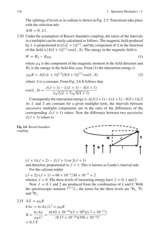
2.50 Under the assumption of Russel–Saunders coupling, the ratios of the intervals
in a multiplet can be easily calculated as follows. The magnetic field produced
by L is proportional to [L(L + 1)]1/2
, and the component of S in the direction
of this field is [S(S + 1)]1/2
cos(L, S). The energy in the magnetic field is
W = W0 − BμB (1)
where μB is the component of the magnetic moment in the field direction and
W0 is the energy in the field-free case. From (1) the interaction energy is
μB B = A[L(L + 1)]1/2
[S(S + 1)]1/2
cos(L, S) (2)
where A is a constant. From Fig. 2.6 It follows that
cos(L, S) =
J(J + 1) − L(L + 1) − S(S + 1)
2
√
L(L + 1)
√
S(S + 1)
Consequently the interaction energy is A[J(J +1)−L(L +1)−S(S+1)]/2
As L and S are constant for a given multiplet term, the intervals between
successive multiplet components are in the ratio of the differences of the
corresponding J(J + 1) values. Now the difference between two successive
J(J + 1) values is
Fig. 2.6 Russel-Saunders
coupling
(J + 1)(J + 2) − J(J + 1) or 2(J + 1)
and therefore proportional to J + 1. This is known as Lande’s interval rule.
For the calcium triplet
(J + 2)/(J + 1) = 60 × 10−4
/30 × 10−4
= 2
whence J = 0. The three levels of increasing energy have J = 0, 1 and 2.
Now J = 0, 1 and 2 are produced from the combination of L and S. With
the spectroscopic notation 2S+1
LJ the terms for the three levels are 3
P0, 3
P1
and 3
P2.
2.51 ΔE = μB B
hΔv = hcΔλ/λ2
= μB B
B =
hcΔλ
μBλ2
=
(6.63 × 10⁻³⁴
)(3 × 10⁸
)(1.7 × 10⁻¹²
)
(9.17 × 10⁻²⁴)(350 × 10−9)2
= 0.3 T](https://image.slidesharecdn.com/1000-solved-problems-in-modern-physics-220626164600-18e7ea67/85/1000-solved-problems-in-modern-physics-pdf-149-320.jpg)
![2.3 Solutions 121
deciding the model of the nucleus, that is discarding the electron–proton
hypothesis. Consider the nitrogen nucleus. The electron–proton hypothesis
implies 14 prorons+7 electrons. This means that it must have odd spin because
the total number of particles is odd (21) and Fermi statistics must be obeyed.
In the neutron–proton model the nitrogen nucleus has 7n + 7p = 14 parti-
cles (even). Therefore Bose statistics must be obeyed. If the electronic wave
function for the molecules is symmetric it was shown that the interchange of
nuclei produces a factor (−1)J
(J = rotational quantum number) in the total
wave function of the molecule. Thus, if the nuclei obey Bose statistics sym-
metric nuclear spin function must be combined with even J rotational states
and antisymmetric with odd J. Because of the statistical weight attached to
spin states, the intensity of even rotational lines will be (I + 1)/I as great
as that of neighboring odd rotational lines where I is the nuclear spin. For
Fermi statistics of the nuclei the spin and rotational states combine in a manner
opposite to that stated previously, the odd rotational lines being more intense
in the ratio (I + 1)/I. The experimental ratio (I + 1)/I = 2 for even to odd
lines, giving I = 1, is consistent with the neutron–proton model.
2.60 The vibrational energy level is
En =
n +
1
2
ω, n = 0, 1, 2 . . .
with ω =
√
(k/μ), k being the force constant and μ the reduced mass of the
oscillating atoms.
μ =
mcm0
mc + m0
=
12 × 16
12 + 16
= 6.857 amu
ω =
1908
6.857 × 1.67 × 10−27
1/2
= 4.082 × 10¹⁴
S−1
Number of molecules in state En is proportional to exp(−nω/kT ), k being
the Boltzmann constant and T the Kelvin temperature. The probability that
the molecule is in the first excited state is
P1 =
exp(−ω/kT )
∞
0 exp(−nω/kT )
= exp(−ω/kT )[1 − exp(−ω/kT )]
ω
kT
=
1.054 × 10−34
× 4.082 × 1014
1.38 × 10−23 × 1, 000
= 3.1177
Therefore, P1 = exp(−3.117)[1 − exp(−3.1177)]
= 0.042
2.61 The rotational energy state is given by
EJ = J
(J + 1)2
2I
, J = 0, 1, 2 . . .
The state with quantum number J is proportional to (2J + 1) exp(−EJ /kT )
The factor (2J + 1) arises from the J state.
N0/N1 = (1/3) exp
2
/IokT](https://image.slidesharecdn.com/1000-solved-problems-in-modern-physics-220626164600-18e7ea67/85/1000-solved-problems-in-modern-physics-pdf-152-320.jpg)
![2.3 Solutions 123
EJ = [J(J + 1)2
c2
]/(2)(0.5)(Mpc2
)r2
E2 = (2)(3)(197.3)2
(10−15
)2
/(940) × (10−10
)2
= 0.264 × 10⁻¹⁰
MeV
= 2.64 × 10⁻⁵
eV
2.65 ΔEJ =
J2
Io
=
J2
μr2
ΔEJ = hc/λ
∴ λ ∝ μ
λ1
λ2
=
0.00260
0.00272
=
μ1
μ2
(1)
μ1 =
16 × 12
16 + 12
; μ2 =
16x
16 + x
(2)
Using (2) in (1) and solving for x, we get x = 13.004. Hence the mass
number is 13.
2.66 En = ω
n +
1
2
=
0
k
μ
n +
1
2
4.5 =
1.054 × 10⁻³⁴
1.6 × 10⁻¹⁹
573
0.5 × 1.67 × 10−27
1/2
n +
1
2
whence n = 7.75
Therefore the molecule would dissociate for n = 8.
2.3.7 Commutators
2.67 (a) Writing x = i
∂
∂p
eipα/
i
∂
∂p
e−ipα/
ψ|p|
= i eip α/
−
iα
e
ipα
ψ(p) + e−ipα/ ∂ψ(p)
∂p
= α +
i ∂ψ(p)
∂p
= α + x
(b) If A and B are Hermitian
(AB)†
= B†
A†
= B A
If the product is to be Hermitian then (AB)†
= AB i.e. AB = B A. Thus,
A and B must commute with each other.](https://image.slidesharecdn.com/1000-solved-problems-in-modern-physics-220626164600-18e7ea67/85/1000-solved-problems-in-modern-physics-pdf-154-320.jpg)
![124 2 Quantum Mechanics – I
2.68 (a) Let f = ei A
; then f †
=
ei A
†
= e−i A
Therefore f †
f = e−i A
ei A
= 1
Thus ei A
is unitary.
(b) (a) Momentum (b) Parity
2.69 (a) exp(iσx θ) = 1 + iσx θ + (iσx θ)2
/2! + (iσx θ)3
/3! + · · ·
= (1 − θ2
/2! + θ4
/4! . . .) + iσx (θ − θ3
/3! + θ5
/5!. . . .)
= cos θ + iσx sin θ
(where we have used the identity σ2
x = 1)
(b)
ϕ∗
(dψ/dx)dx = ϕ∗
ψ −
(dϕ∗
/dx)ψdx
But ϕ∗
ψ = 0
Hence
ϕ∗
dψ
dx
dx =
−dϕ∗
dx
ψdx =
−(dϕ/dx)†
ψdx
Therefore
d
dx
†
= −d/dx
2.70 (a) [x, Px ]ψ = x Px ψ − Px xψ
= x
−i
∂
∂x
ψ + i
∂
∂x
(xψ)
= −ix
∂ψ
∂x
+ ix
∂ψ
∂x
+ iψ
= iψ
∴ [x, Px ] = i
(b) [x2
, Px ]ψ = x2
(−i∂ ψ/∂x + i
∂
∂x
(x2
ψ)
= −ix2
∂ ψ/∂x + i x2
∂ψ/∂x + i(2x)ψ
= 2ixψ
Therefore [x2
, px ] = 2ix
2.71 By definition a transformation A is said to be linear if for any constant (possi-
bly complex) λ
A(λX) = λ A X
And if for any two vectors x and y
A(x + y) = Ax + Ay
If H is a hermitian operator
(x, Hλy) = (Hx, λy) = λ(Hx, y) = λ(x, Hy) = (x, λHy)
Or Hλy = λHy
for any y. Furthermore
(z, H(x + y)) = (Hz, x + y) = (Hz, x) + (Hz, y)
= (z, Hx) + (z, Hy) = (z, Hx + Hy)
∴ H(x + y) = Hx + Hy
2.72 Consider the equation
∂
∂x
(ψ∗
ψ) = ψ∗ ∂ψ
∂x
+ ψ
dψ∗
dx
(1)](https://image.slidesharecdn.com/1000-solved-problems-in-modern-physics-220626164600-18e7ea67/85/1000-solved-problems-in-modern-physics-pdf-155-320.jpg)
![2.3 Solutions 125
Integration of (1) yields
∂
∂x
(ψ∗
ψ)dτ +
ψ∗ ∂ψ
∂x
dτ +
ψ
dψ∗
dx
dτ (2)
The integral on the LHS vanishes because ψ∗
ψ vanishes for large values of
|x| if the particle is confined to some finite region. Thus
∂
∂x
(ψ∗
ψ)dxdydz =
|ψ∗
ψ|∞
−∞dydz = 0
Therefore (2) becomes
ψ∗
∂ψ
∂x
dτ = −
ψ
∂ψ∗
∂x
dτ (3)
Generalizing to all the three coordinates
(ψ, ∇ψ) = −(∇ψ, ψ) (4)
Hence
(ψ, i∇ψ) = (i∇ψ, ψ) (5)
where we have used, i∇ψ, ψ = −
i∇ ψ∗
ψ dτ.
This completes the proof that the momentum operator is hermitian.
2.73 Using the standard method explained in Chap. 1, define the eigen values
λ1 = 3 and λ2 = −1 for the matrix P and the eigen vectors 1
√
2
1
1
and
1
√
2
1
−1
. For the matrix Q, the eigen values are λ1 = 5 and λ2 = 1, the eigen
vectors being 1
√
2
1
1
and 1
√
2
1
−1
. Thus the eigen vectors for the commutat-
ing matrices are identical.
2.74 (a) A = αx + iβp
A†
= ax†
− iβp†
(b)[A, x] = α[x, x] + iβ[p, x]
= 0 + iβ(−i) = β
[A, A] = AA − AA = 0
[A, p] = α[x, p] + iβ[p, p]
= iα + 0 = iα
2.75 (a) As A satisfies a quadratic equation it can be represented by a 2 × 2 matrix.
Its eigen values are the roots of the quadratic equation
λ2
− 4λ + 3 = 0, λ1 = 1, λ2 = 3
(b) A is represented by the matrix
A =
1 0
0 3
The eigen value equation is
1 0
0 3
a
b
= λ
a
b](https://image.slidesharecdn.com/1000-solved-problems-in-modern-physics-220626164600-18e7ea67/85/1000-solved-problems-in-modern-physics-pdf-156-320.jpg)
![126 2 Quantum Mechanics – I
This gives a = 1, b = 0 for λ = 1 and a = 0, b = 1 for λ = 3
Hence the eigen states of A are
1
0
and
0
1
(c) As A = A†
, A is Hermitian and hence an observable.
2.76 (a) A general rule for commutators is
[A2
, B] = A[A, B] + [A, B]A
Here H = P2
/2μ
[H, X] = (1/2μ)[P2
, x] = (1/2μ)(P[P, x] + [P, x]P)
= (1/2μ)2p/i = p/iμ
Therefore [x, H] = ip/μ
(b) [[x, H], x] =
iPx
μ
, x
=
i
μ
[Px , x] =
i
μ
(−i) =
2
μ
2.77 [A2
, B] = A A B − B A A = A A B − A B A + A B A − B A A
= A[A, B] + [A, B]A
2.78 (σ.A)(σ.B) = (σx Ax + σy Ay + σz Az)(σx Bx + σy By + σz Bz)
= Ax Bx σ2
x + Ay Byσ2
y + Az Bzσ2
z + σx σy Ax By + σx σz Ax Bz
+ σyσx Ay Bx + σyσz Ay Bz + σzσx Az Bx + σzσy Az By
= A.B + iσz(Ax By − Ay Bx ) + iσx (Ay Bz − Az By)
+ iσy(Az Bx − Bz Ax )
= A.B + i[σ.(A × B)]z + i[σ.(A × B)]x + i[σ.(A × B)]y
= A.B + i σ.(A × B)
where we have used the identities in simplifying:
σ2
x = σ2
y = σ2
z = 1
and σyσx = −σx σy etc.
2.79 (a) σyμ = σμy† as can be seen from the matrix elements of σy. Therefore σy is
Hermitian. It is the matrix of a Hermitian operator whose eigen values are
real.
(b) The eigen values λ are found by setting
%
%
%
%
σ y11 −λ σ y11
σ y21 σ y22 −λ
%
%
%
% =
%
%
%
%
−λ −i
i −λ
%
%
%
% = 0
λ2
− 1 = 0, λ = ±1](https://image.slidesharecdn.com/1000-solved-problems-in-modern-physics-220626164600-18e7ea67/85/1000-solved-problems-in-modern-physics-pdf-157-320.jpg)
![2.3 Solutions 127
The eigen vector associated with λ1 = 1 is
|ψ1 =
2
n=1
Cn|n with − C1 − iC2 = 0, C2 = iC1,
|ψ1 =
1
√
2
|1 +
i
√
2
|2
The eigen vector associated with λ2 = −1 is
|ψ2 =
2
n=1
Cn|n with C1 − iC2 = 0, C2 = −iC1,
|ψ2 =
1
√
2
|1 −
i
√
2
|2
(c) The projector onto |ψi is Pi = |ψi ψi |.
Matrix of P1 =
1
2
− i
2
i
2
1
2
'
, matrix of P2 =
1
2
i
2
− i
2
1
2
'
P1
†
P2
0 0
0 0
= 0, P1 P1
†
+ P2 P2
†
= I
2.80 (i) σx
2
=
0 1
1 0
0 1
1 0
=
1 0
0 1
(ii) [σx , σy] =
0 1
1 0
0 −i
i 0
−
0 −i
i 0
0 1
1 0
=
i 0
0 −i
−
−i 0
0 i
=
2i 0
0 −2i
= 2i
1 0
0 −1
= 2iσz
2.81 Proof : A X = λ1 X (1)
BX = λ2 X (2)
where λ1 and λ2 are the eigen values belonging to the same state λ.
B AX = Bλ1 X = λ1 BX = λ1λ2 X (3)
ABX = Aλ2 X = λ2 AX = λ2λ1 X = λ1λ2 X (4)
Subtracting (3) from (4)
(A B − B A)X = 0
Therefore A B − B A = 0, because X
= 0
Operate with B on A in (1) and with A and B in (2)
Or [A, B] = 0](https://image.slidesharecdn.com/1000-solved-problems-in-modern-physics-220626164600-18e7ea67/85/1000-solved-problems-in-modern-physics-pdf-158-320.jpg)
![128 2 Quantum Mechanics – I
2.3.8 Uncertainty Principle
2.82 ΔxΔpx∼/2
P =
2x
E =
p2
2m
+ 1/2 mω2
x2
=
2
8mx2
+ 1/2mω2
x2
The ground state energy is obtained by setting ∂E
∂x
= 0
∂E
∂x
= −
2
4mx3
+ mω2
x = 0
whence x2
=
2mω
∴ E = 1/4ω + 1/4ω = 1
2
ω
2.83 If E and p are to be measured simultaneously their operators must commute.
Now
H = −2
∇2
/2m + V and p = −i∇
[H, p] = [−2
∇2
/2m + V, −i∇]
= i3
∇2
∇/2m − iV ∇ − i3
∇∇2
/2m + i∇V
The first and the third term on the RHS get cancelled because ∇2
∇ = ∇∇2
.
Therefore
[H, P] = −i(V ∇ − ∇V )
If V = constant, the commutator vanishes. To put it differently energy
and momentum can be measured with arbitrary precision only for unbound
particles.
2.84 Consider the motion of a particle along x-direction.
The uncertainty Δx is defined as
(Δx)2
= (x− x )2
= x2
−2 x x + x 2
= x2
− x 2
(1)
Similarly
(ΔPx )2
= P2
x − Px 2
(2)](https://image.slidesharecdn.com/1000-solved-problems-in-modern-physics-220626164600-18e7ea67/85/1000-solved-problems-in-modern-physics-pdf-159-320.jpg)
![2.3 Solutions 129
The precise statement of the Heisenberg uncertainty principle is
ΔPx Δx ≥ /2
ΔPyΔy ≥ /2 (3)
ΔPzΔz ≥ /2
Consider the integral, a function of a real parameter λ
I(λ) =
∞
−∞
dx|(x− x )ψ + iλ(−i∂ψ/∂x− Px ψ|2
(4)
By definition, I(λ ≥ 0). Expanding (4)
I(λ) =
∞
−∞
dxψ∗
(x− x )2
ψ + λ
∞
−∞
dx
ψ∗ ∂ψ
∂x
+ ψ
∂ψ∗
∂x
(x− x )
+ λ2
2
∞
−∞
∂ψ∗
∂x
∂ψ
∂x
− iλ2
Px
∞
−∞
dx[ψ
∂ψ∗
∂x
+ λ2
Px 2
∞
−∞
dxψ∗
ψ (5)
The term in the second line can be written as
∞
−∞
dx
∂
∂x
(ψ∗
ψ)(x− x ) = [(x− x )ψ∗
ψ]∞
−∞ −
∞
−∞
dxψ∗
ψ = −1
because it is expected that ψ → 0. Sufficiently fast as x → ±∞ so that the
integrated term is zero. Similarly the third term can be re-written as
2
∞
−∞
dx
∂ψ∗
∂x
∂ψ
∂x
= 2
ψ∗ ∂ψ
∂x
∞
−∞
+
∞
−∞
dxψ∗
(−2
∂2
ψ/∂x2
) = P2
x
In term (4) rewrite
−i
∞
−∞
dx
∂ψ∗
∂x
ψ = −i
,
ψ∗
ψ
-∞
−∞
+
∞
−∞
dxψ∗
i
∂ψ
∂x
= − Px
So, the full term (4) becomes −2 Px 2
.
Collecting all the terms
I(λ) = (Δx)2
− λ + (ΔPx )2
λ2
≥ 0
Denoting I(λ) = aλ2
+ bλ + c, the condition I(λ ≥ 0) is satisfied if
b2
− 4ac ≥ 0.
Thus, 2
− 4(Δx)2
(ΔPx )2
≤ 0, and therefore
ΔPx Δx ≥ /2
2.85 ΔxΔp =
cΔP ≈ cp =
c
Δx
=
197.3MeV − fm
0.529 × 10⁻¹⁰ m
= 372.97 × 10⁻⁵
MeV = 3,730 eV
T = c2
p2
/mc2
= (3,730)2
/0.511 × 106
= 13.61 eV](https://image.slidesharecdn.com/1000-solved-problems-in-modern-physics-220626164600-18e7ea67/85/1000-solved-problems-in-modern-physics-pdf-160-320.jpg)
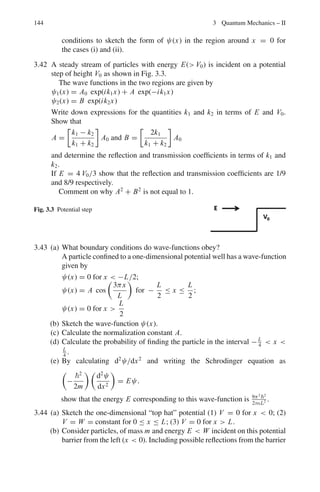
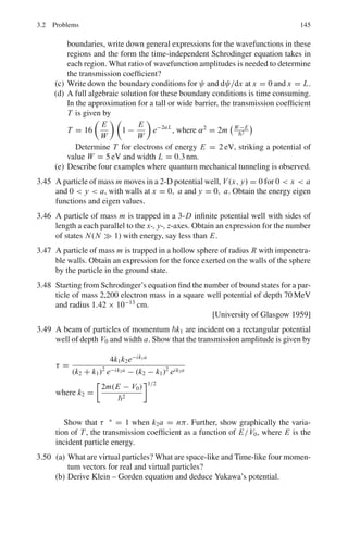
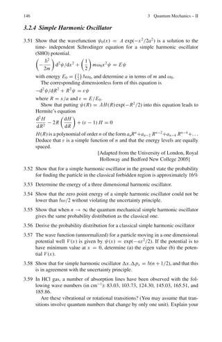
![3.1 Basic Concepts and Formulae 133
Commutators
AB − BA = [A, B] (3.12)
by definition.
Dirac’s Bra and Ket notation
A ket vector, or simply ket, is analogous to the wave function for a state. The symbol
|m denotes the ket vector that corresponds to the state m of the system. A bra
vector, or bra, is analogous to the complex conjugate of the wave function for a
state. The symbol n| denotes the bra vector that corresponds to the state n of the
system. Then
ψ∗
n ψm dτ =](https://image.slidesharecdn.com/1000-solved-problems-in-modern-physics-220626164600-18e7ea67/85/1000-solved-problems-in-modern-physics-pdf-164-320.jpg)
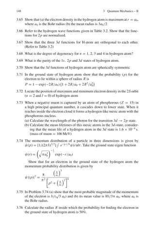
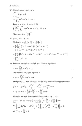
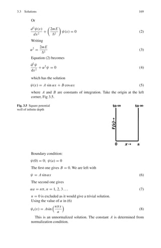
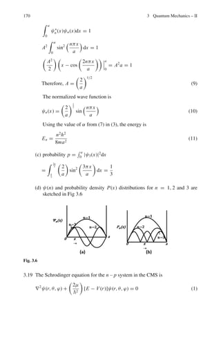
![138 3 Quantum Mechanics – II
3.8 (a) State and explain Laporte rule for light emission.
(b) What are metastable states?
3.9 Show that the eigen values of a hermitian operator Q are real
3.10 The state of a free particle is described by the following wave function
(Fig. 3.1)
ψ(x) = 0 for x −3a
= c for − 3a x a
= 0 for x a
(a) Determine c using the normalization condition
(b) Find the probability of finding the particle in the interval [0, a]
Fig. 3.1 Uniform distribution
of ψ
3.11 In Problem 3.10,
(a) Compute x and σ2
(b) Calculate the momentum probability density.
3.12 Particle is described by the wavefunction
ψ = 0 x 0
=
√
2e−x/L
x ≥ 0
where L = 1 nm. Calculate the probability of finding the particle in the region
x ≥ 1 nm.
3.2.2 Schrodinger Equation
3.13 The radial Schrodinger equation, in atomic units, for an electron in a hydrogen
atom for which the orbital angular momentum quantum number, l = 0, is
((d2
/dr2
) + (2/r) + (2E))F(r) = 0,
where E is the total energy.](https://image.slidesharecdn.com/1000-solved-problems-in-modern-physics-220626164600-18e7ea67/85/1000-solved-problems-in-modern-physics-pdf-188-320.jpg)
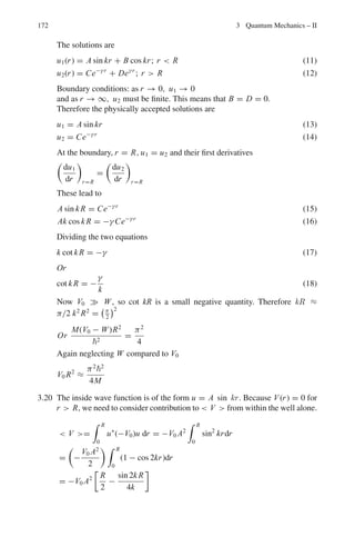
![140 3 Quantum Mechanics – II
3.17 In Problem 3.16,
(a) Consider the case where m = 0. Make the change of variable μcos θ and
consider a series solution to the equation for (μ). Derive a recurrence rela-
tion for the coefficients of the series solution.
(b) Explain why the series solution should be cut off at some finite term, give
a mechanism for doing this and hence derive another quantum number l.
3.2.3 Potential Wells and Barriers
3.18 (a) The one-dimensional time-independent Schrodinger equation is
−
2
2m
d2
ψ(x)
dx2
+ U(x)ψ(x) = Eψ(x)
Give the meanings of the symbols in this equation.
(b) A particle of mass m is contained in a one-dimensional box of width a.
The potential energy U(x) is infinite at the walls of the box (x = 0 and
x = a) and zero in between (0 x a).
Solve the Schrodinger equation for this particle and hence show that the
normalized solutions have the form ψn(x) =
2
a
1
2
sin
nπx
a
, with energy
En = h2
n2
/8ma2
, where n is an integer (n 0).
(c) For the case n = 3, find the probability that the particle will be located in
the region a
3
x 2a
3
.
(d) Sketch the wave-functions and the corresponding probability density dis-
tributions for the cases n = 1, 2 and 3.
3.19 Deuteron is a loose system of neutron and proton each of mass M. Assuming
that the system can be described by a square well of depth V0 and width R,
show that to a good approximation
V0 R2
=
π
2
2
2
M
3.20 Show that the expectation value of the potential energy of deuteron described
by a square well of depth V0 and width R is given by
V = −V0 A2
R
2
−
sin 2kR
4k
where A is a constant.
3.21 Assuming that the radial wave function
U(r) = rψ(r) = C exp(−kr)
is valid for the deuteron from r = 0 to r = ∞ find the normalization
constant C.
Hence if k = 0.232 fm−1
find the probability that the neutron – proton separa-
tion in the deuteron exceeds 2 fm. Find also the average distance of interaction
for this wave function.
[Royal Holloway University of London 1999]](https://image.slidesharecdn.com/1000-solved-problems-in-modern-physics-220626164600-18e7ea67/85/1000-solved-problems-in-modern-physics-pdf-190-320.jpg)
![3.2 Problems 141
3.22 The small binding energy of the deuteron (2.2 MeV) implies that the maximum
of U(r) lies just inside the range R of the well. From this knowledge deduce
the value of V0 if R is approximately 1.5 fm.
[Osmania University]
3.23 Given that the normalized wave function
ψ =
1
r
α
2π
1/2
e−αr
(1/α = 4.3 fm) is a useful approximation to describe the ground state of the
deuteron, find the root mean square separation of the neutron and proton in
this nucleus.
[University of Durham 1972]
3.24 A particle of mass me trapped in an infinite depth well of width L = 1 nm.
Consider the transition from the excited state n = 2 to the ground state n = 1.
Calculate the wavelength of light emitted. In which region of electromagnetic
spectrum does it fall?
3.25 Consider a particle of mass m trapped in a potential well of finite depth V0
V (x) = V0, |x| a
= 0; |x| a
Discuss the solutions and eigen values for the class I and II solutions graphi-
cally.
3.26 Show that for deuteron, neutron and proton stay outside the range of nuclear
forces for 70% of the time. Take the binding energy of deuteron as 2.2 MeV.
3.27 Show that the results of the energy levels for infinite well follow from those
for the finite well.
3.28 Show that for deuteron excited states are not possible.
3.29 The small binding energy of the deuteron indicates that the maximum of U(r)
lies only just inside the range R of the square well potential. Use this informa-
tion to estimate the value of V0 if R is approximately 1.5 fm.
3.30 Consider a stream of particles with energy E travelling in one dimension from
x = −∞ to ∞. The particles have an average spacing of distance L. The
particle stream encounters a potential barrier at x = 0. The potential can be
written as
V (x) = 0 if x 0
= V if 0 x a
= 0 if x a
Suppose the particle energy is smaller than the potential barrier, i.e., Vb.
(a) For each of the three regions, write down Schrodinger’s equation and cal-
culate the wave-function ψ and its derivative dψ/dx.](https://image.slidesharecdn.com/1000-solved-problems-in-modern-physics-220626164600-18e7ea67/85/1000-solved-problems-in-modern-physics-pdf-191-320.jpg)
![142 3 Quantum Mechanics – II
Use the constants to represent the amplitude of the reflected and trans-
mitted particle streams respectively and take
k2
1 =
2mE
2
and k2
2 =
2m(Vb − E)
2
(b) At the boundaries to the potential barrier, ψ and dψ/dx must be continu-
ous. Equate the solutions that you have at x = 0 and x = a and manipulate
these equations to derive the following expression for the transmission
amplitude
τ =
4ik1k2e−ik1a
[(ik1 + k2)2e−k2a] − [(ik1 − k2)2ek2a]
3.31 In Problem 3.30,
(a) Show that the fraction of transmitted particles is given by Ftrans = τ∗
τ,
which when calculated evaluates to
Ftrans =
1 +
V2
b sinh2
(k2a)
4E(Vb − E)
'−1
(b) How would Ftrans vary if E Vb.
3.32 A particle is trapped in a one dimensional potential given by = kx2
/2. At a
time t = 0 the state of the particle is described by the wave function ψ =
C1ψ1 + C2ψ2, where ψ is the eigen function belonging to the eigen value En.
What is the expected value of the energy?
3.33 A particle is trapped in an infinitely deep square well of width a. Sud-
denly the walls are separated by infinite distance so that the particle becomes
free. What is the probability that the particle has momentum between p and
p + dp?
3.34 The alpha decay is explained as a quantum mechanical tunneling. Assuming
that the alpha particle energy is much smaller than the potential barrier the
alpha particle has to penetrate, the transmission coefficient is given by
T ≈ exp
−
2
b
a
[2m(U(r) − E)]1/2
dr
The integration limits a and b are determined as solutions to the equation
U(r) = E, where U(r) is the non-constant Coulomb’s potential energy. Cal-
culate the alpha transmission coefficient and the decay constant λ.
3.35 The one-dimensional square well shown in Fig. 3.2 rises to infinity at x = 0
and has range a and depth V1. Derive the condition for a spinless particle of
mass m to have (a) barely one bound state (b) two and only two bound states
in the well. Sketch the wave function of these two states inside and outside the
well and give their analytic expressions.](https://image.slidesharecdn.com/1000-solved-problems-in-modern-physics-220626164600-18e7ea67/85/1000-solved-problems-in-modern-physics-pdf-192-320.jpg)
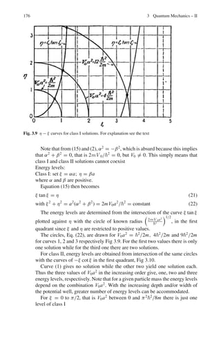
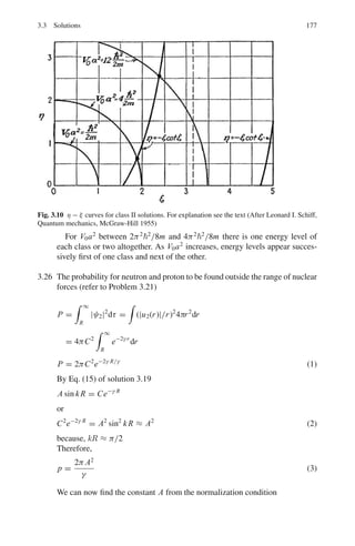
![3.2 Problems 145
boundaries, write down general expressions for the wavefunctions in these
regions and the form the time-independent Schrodinger equation takes in
each region. What ratio of wavefunction amplitudes is needed to determine
the transmission coefficient?
(c) Write down the boundary conditions for ψ and dψ/dx at x = 0 and x = L.
(d) A full algebraic solution for these boundary conditions is time consuming.
In the approximation for a tall or wide barrier, the transmission coefficient
T is given by
T = 16
E
W
1 −
E
W
e−2αL
, where α2
= 2m
W−E
2
Determine T for electrons of energy E = 2 eV, striking a potential of
value W = 5 eV and width L = 0.3 nm.
(e) Describe four examples where quantum mechanical tunneling is observed.
3.45 A particle of mass m moves in a 2-D potential well, V (x, y) = 0 for 0 x a
and 0 y a, with walls at x = 0, a and y = 0, a. Obtain the energy eigen
functions and eigen values.
3.46 A particle of mass m is trapped in a 3-D infinite potential well with sides of
length a each parallel to the x-, y-, z-axes. Obtain an expression for the number
of states N(N 1) with energy, say less than E.
3.47 A particle of mass m is trapped in a hollow sphere of radius R with impenetra-
ble walls. Obtain an expression for the force exerted on the walls of the sphere
by the particle in the ground state.
3.48 Starting from Schrodinger’s equation find the number of bound states for a par-
ticle of mass 2,200 electron mass in a square well potential of depth 70 MeV
and radius 1.42 × 10⁻¹³
cm.
[University of Glasgow 1959]
3.49 A beam of particles of momentum k1 are incident on a rectangular potential
well of depth V0 and width a. Show that the transmission amplitude is given by
τ =
4k1k2e−ik1a
(k2 + k1)2
e−ik2a − (k2 − k1)2
eik2a
where k2 =
2m(E − V0)
2
1/2
Show that τ ∗
= 1 when k2a = nπ. Further, show graphically the varia-
tion of T , the transmission coefficient as a function of E/V0, where E is the
incident particle energy.
3.50 (a) What are virtual particles? What are space-like and Time-like four momen-
tum vectors for real and virtual particles?
(b) Derive Klein – Gorden equation and deduce Yukawa’s potential.](https://image.slidesharecdn.com/1000-solved-problems-in-modern-physics-220626164600-18e7ea67/85/1000-solved-problems-in-modern-physics-pdf-195-320.jpg)
![146 3 Quantum Mechanics – II
3.2.4 Simple Harmonic Oscillator
3.51 Show that the wavefunction ψ0(x) = A exp(−x2
/2a2
) is a solution to the
time- independent Schrodinger equation for a simple harmonic oscillator
(SHO) potential.
−
2
2m
d2
ψ/dx2
+
1
2
mω0x2
ψ = Eψ
with energy E0 =
1
2
ω0, and determine a in terms of m and ω0.
The corresponding dimensionless form of this equation is
−d2
ψ/dR2
+ R2
ψ = εψ
where R = x/a and ε = E/E0.
Show that putting ψ(R) = AH (R) exp(−R2
/2) into this equation leads to
Hermite’s equation
d2
H
dR2
− 2R
dH
dR
+ (ε − 1) H = 0
H(R) is a polynomial of order n of the form anRn
+an−2 Rn−2
+an−4 Rn−4
+. . .
Deduce that ε is a simple function of n and that the energy levels are equally
spaced.
[Adapted from the University of London, Royal
Holloway and Bedford New College 2005]
3.52 Show that for a simple harmonic oscillator in the ground state the probability
for finding the particle in the classical forbidden region is approximately 16%
3.53 Determine the energy of a three dimensional harmonic oscillator.
3.54 Show that the zero point energy of a simple harmonic oscillator could not be
lower than ω/2 without violating the uncertainty principle.
3.55 Show that when n → ∞ the quantum mechanical simple harmonic oscillator
gives the same probability distribution as the classical one.
3.56 Derive the probability distribution for a classical simple harmonic oscillator
3.57 The wave function (unnormalized) for a particle moving in a one dimensional
potential well V (x) is given by ψ(x) = exp(−ax2
/2). If the potential is to
have minimum value at x = 0, determine (a) the eigen value (b) the poten-
tial V (x).
3.58 Show that for simple harmonic oscillator Δx.Δpx = (n + 1/2), and that this
is in agreement with the uncertainty principle.
3.59 In HCl gas, a number of absorption lines have been observed with the fol-
lowing wave numbers (in cm−1
): 83.03, 103.73, 124.30, 145.03, 165.51, and
185.86.
Are these vibrational or rotational transitions? (You may assume that tran-
sitions involve quantum numbers that change by only one unit). Explain your](https://image.slidesharecdn.com/1000-solved-problems-in-modern-physics-220626164600-18e7ea67/85/1000-solved-problems-in-modern-physics-pdf-196-320.jpg)
![3.2 Problems 147
reasoning briefly. (a) If the transitions are vibrational, estimate the spring con-
stant (in dyne/cm) (b) If the transitions are rotational, estimate the separation
between H and Cl nuclei. What J values do they correspond to, and what is
the moment of inertia of HCl (in g-cm2
)?
[Arizona State University 1996]
3.60 Determine the degeneracy of the energy levels of an isotropic harmonic oscil-
lator.
3.61 At time t = 0, particle in a harmonic oscillator potential V (x) = mω2
x2
2
has a
wavefunction
ψ(x, 0) =
1
√
2
[ψ0(x) + ψ1(x)]
where ψ0(x) and ψ1(x) are real ortho-normal eigen functions for the ground
and first-excited states of the oscillator. Show that the probability density
|ψ(x, t)|2
oscillates with angular frequency ω.
3.62 The quantum state of a harmonic oscillator has the eigen-function ψ(x, t) =
1
√
2
ψ0(x) exp
−
i E0t
+
1
√
3
ψ1(x) exp
−
i E1t
+
1
√
6
ψ2(x) exp
−
i E2t
where ψ0(x), ψ1(x) and ψ2(x) are real normalized eigen functions of the har-
monic oscillator with energy E0, E1 and E2 respectively. Find the expectation
value of the energy.
3.63 (a) Show that the wave-function ψ0(x) = A exp(−x2
/2a2
) with energy E =
ω/2 (where A and a are constants) is a solution for all values of x to the
one-dimensional time-independent Schrodinger equation (TISE) for the
simple harmonic oscillator (SHO) potential V (x) = mω2
x2
/2
(b) Sketch the function ψ1(x) = Bx exp(−x2
/2a2
)
(where B = constant), and show that it too is a solution of the TISE for
all values of x.
(c) Show that the corresponding energy E = (3/2)ω
(d) Determine the expectation value px of the momentum in state ψ1
(e) Briefly discuss the relevance of the SHO in describing the behavior of
diatomic molecules.
3.2.5 Hydrogen Atom
3.64 Find the expectation value of kinetic energy, potential energy, and total energy
of hydrogen atom in the ground state. Take ψ0 = e−r/a0
(π a3
0 )1/2 , where a0 = Bohr’s
radius](https://image.slidesharecdn.com/1000-solved-problems-in-modern-physics-220626164600-18e7ea67/85/1000-solved-problems-in-modern-physics-pdf-197-320.jpg)
![148 3 Quantum Mechanics – II
3.65 Show that (a) the electron density in the hydrogen atom is maximum at r = a0,
where a0 is the Bohr radius (b) the mean radius is 3a0/2
3.66 Refer to the hydrogen wave functions given in Table 3.2. Show that the func-
tions for 2p are normalized.
3.67 Show that the three 3d functions for H-atom are orthogonal to each other.
(Refer to Table 3.2)
3.68 What is the degree of degeneracy for n = 1, 2, 3 and 4 in hydrogen atom?
3.69 What is the parity of the 1s, 2p and 3d states of hydrogen atom.
3.70 Show that the 3d functions of hydrogen atom are spherically symmetric
3.71 In the ground state of hydrogen atom show that the probability (p) for the
electron to lie within a sphere of radius R is
P = 1 − exp (−2R/a0)
1 + 2R/a0 + 2R2
/a2
0
3.72 Locate the position of maximum and minimum electron density in the 2S orbit
(n = 2 and l = 0) of hydrogen atom
3.73 When a negative muon is captured by an atom of phosphorous (Z = 15) in
a high principal quantum number, it cascades down to lower state. When it
reaches inside the electron cloud it forms a hydrogen-like mesic atom with the
phosphorous nucleus.
(a) Calculate the wavelength of the photon for the transition 3d → 2p state.
(b) Calculate the mean lifetimes of this mesic atoms in the 3d-state, consider-
ing that the mean life of a hydrogen atom in the 3d state is 1.6 × 10⁻⁸
s.
(mass of muon = 106 MeV)
3.74 The momentum distribution of a particle in three dimensions is given by
ψ(p) = [1/(2π)3/2
]
e−p.r/
ψ(r)dτ. Take the ground state eigen function
ψ(r) =
$
πa3
0
− 1
2
exp (−r/a0)
Show that for an electron in the ground state of the hydrogen atom the
momentum probability distribution is given by
ψ|(p)|2
=
8
π2
a0
5
p2 +
a0
2
4
3.75 In Problem 3.74 (a) show that the most probable magnitude of the momentum
of the electron is /(
√
3 a0) and (b) its mean value is 8/3π a0, where a0 is
the Bohr radius.
3.76 Calculate the radius R inside which the probability for finding the electron in
the ground state of hydrogen atom is 50%.](https://image.slidesharecdn.com/1000-solved-problems-in-modern-physics-220626164600-18e7ea67/85/1000-solved-problems-in-modern-physics-pdf-198-320.jpg)
![3.2 Problems 149
3.2.6 Angular Momentum
3.77 Given that L = r × p, show that [Lx , Ly] = iLz
3.78 The spin wave function of two electrons is (x ↑ x ↓ –x ↓ x ↑)/
√
2. What is
the eigen value of S1.S2? S1 and S2 are spin operators of 1 and 2 electrons
3.79 Show that for proton – neutron system
σp.σn = −3 for singlet state
= 1 for triplet state
3.80 Write down an expression for the z-component of angular momentum, Lz, of a
particle moving in the (x, y) plane in terms of its linear momentum components
px and py.
Using the operator correspondence px = −i
∂
∂x
etc., show that
Lz = −i
x
∂
∂y
− y
∂
∂x
Hence show that Lz = −i
∂
∂ϕ
, where the coordinates (x,y) and (r, ϕ) are
related in the usual way.
Assuming that the wavefunction for this particle can be written in the form
ψ(r, ϕ) = R(r)Φ(ϕ) show that the z-component of angular momentum is
quantized with eigen value , where m is an integer.
3.81 Show that the operators Lx and Ly in the spherical polar coordinates are
given by
Lx
i
= sin ϕ
∂
∂θ
+ cot θ cos ϕ
∂
∂ϕ
Ly
i
= − cos ϕ
∂
∂θ
+ cot θ sin ϕ
∂
∂ϕ
3.82 Using the commutator [Lx , Ly] = i Lz, and its cyclic variants, prove that
total angular momentum squared and the individual components of angular
momentum commute, i.e [L2
, Lx ] = 0 etc.
3.83 Show that in the spherical polar coordinates
L2
(i)2
=
∂2
∂θ2
+
1
sin2
θ
∂2
∂ϕ2
+ cot θ
∂
∂θ
And show that in the expression for ∇2
in spherical polar coordinates the
angular terms are proportional to L2
.
3.84 (a) Obtain the angular momentum matrices for j = 1/2 particles
(b) Hence Obtain the matrix for J2
.](https://image.slidesharecdn.com/1000-solved-problems-in-modern-physics-220626164600-18e7ea67/85/1000-solved-problems-in-modern-physics-pdf-199-320.jpg)
![150 3 Quantum Mechanics – II
3.85 (a) Obtain the angular momentum matrices for j = 1
(b) Hence obtain the matrix for J2
.
3.86 Two angular momenta with j1 = 1 and j2 = 1/2 are vectorially added, obtain
the Clebsch – Gordan coefficients.
3.87 The wave function of a particle in a spherically symmetric potential is
Ψ (x, y, z) = C (xy + yz + zx)e−αr2
Show that the probability is zero for the angular momentum l = 0 and l = 1
and that it is unity for l = 2
3.88 Show that the states specified by the wave-functions
ψ1 = (x + iy) f (r)
ψ2 = zf (r)
ψ3 = (x − iy) f (r)
are eigen states of the z-component of angular momentum and obtain the cor-
responding eigen values.
[Adapted from the University of Manchester 1959]
3.89 The Schrodinger wave function for a stationary state of an atom is
ψ = Af (r) sin θ cos θeiϕ
where (r, θ, ϕ) are spherical polar coordinates. Find (a) the z component of the
angular momentum of the atom (b) the square of the total angular momentum
of the atom. (You may use the following transformations from Cartesian to
spherical polar coordinates
x
∂
∂y
− y
∂
∂x
= sin ϕ
∂
∂θ
+ cot θ cos ϕ
∂
∂ϕ
x
∂
∂z
− z
∂
∂x
= − cos ϕ
∂
∂θ
+ cot θ sin ϕ
∂
∂ϕ
y
∂
∂x
− x
∂
∂y
= −
∂
∂ϕ
[Adapted from the University of Durham 1963]
3.90 The normalized Schrodinger wavefunctions for one of the stationary states of
the hydrogen atom is given in spherical polar coordinates, by
ψ(r, θ, ϕ) =
1
2a0
3/2
1
√
3
r
a0
exp
−
r
2a0
3
8π
1/2
sin θ exp (−iϕ)
(a) Find the value of the component of angular momentum along the z axis
(θ = 0)
(b) What is the parity of this wavefunction?
[a0 is the radius of the first Bohr orbit]
[Adapted from the University of New Castle 1964]](https://image.slidesharecdn.com/1000-solved-problems-in-modern-physics-220626164600-18e7ea67/85/1000-solved-problems-in-modern-physics-pdf-200-320.jpg)
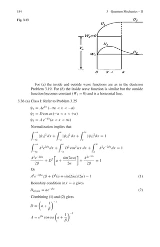
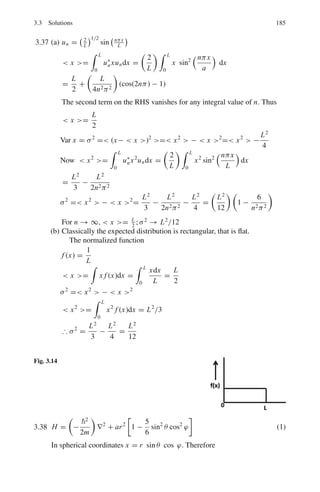
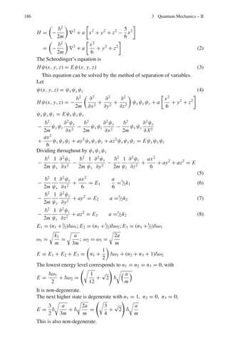
![15
32π
sin2
θ exp (±2iϕ)
[University College, London]
3.94 Given that the complete wave function of a hydrogen-like atom in a particular
state is ψ(r, θ, ϕ) = Nr2
exp
− Zr
3a0
sin2
θ e2iϕ
determine the eigen value of
Lz, the third component of the angular momentum operator.
3.95 Consider an electron in a state described by the wave function
ψ =
1
√
4π
(cosθ + sinθeiϕ
) f (r)
where
∞
0
| f (r)|2
r2
dr = 1
(a) Show that the possible values of Lz are + and zero
(b) Show that the probability for the occurrence of the Lz values in (a) is 2/3
and 1/3, respectively.
3.96 Show that (a) [Jz, J+] = J+ (b) J+|jm = Cjm + | j, m + 1 (c) [Jx , Jy]
= iJ z](https://image.slidesharecdn.com/1000-solved-problems-in-modern-physics-220626164600-18e7ea67/85/1000-solved-problems-in-modern-physics-pdf-205-320.jpg)
![152 3 Quantum Mechanics – II
3.2.7 Approximate Methods
3.97 Consider hydrogen atom with proton of finite size sphere with uniform
charge distribution and radius R. The potential is
V (r) = −
3e2
2R3
(R2
− r2
/3) for r R
= −e2
/r for r R
Calculate correction to first order for n = 1 and n = 2 with l = 0 states
[Adapted from University of Durham 1963]
3.98 A particle of mass m and charge q oscillating with frequency ω is subjected
to a uniform electric field E parallel to the direction of oscillation. Determine
the stationary energy levels.
3.99 Consider the Hermitian Hamiltonian H = H0 + H
, where H
is a small
perturbation. Assume that exact solutions H0|ψ = E0|ψ are known, two
of them, and that they are orthogonal and degenerate in energy. Work out to
first order in H
, the energies of the perturbed levels in terms of the matrix
elements of H
.
3.100 The helium atom has nuclear charge +2e surrounded by two electrons. The
Hamiltonian is
H =
−
2
2m
(∇2
1 + ∇2
2 ) − 2e2
1
r1
+
1
r2
+
e2
r12
where r1 and r2 are the position vectors of the two electrons with nucleus as
the origin, and r12 = |r1 − r2| is the distance between the two electrons. The
expectation value for the first two terms are evaluated in a straight forward
manner, the third term which is the interaction energy of the two electrons is
evaluated by taking the trial function as the product of two hydrogenic wave
functions for the ground state. The result is
H =
e2
Z2
a0
−
4e2
Z
a0
+
5e2
Z
8a0
=
e2
a0
Z2
−
27Z
8
Thus, the energy obtained by the trial function is
E(Z) =
−
e2
2a0
27Z
4
− 2Z2
Determine the ionization energy of the helium atom.
3.101 Consider the first-order change in the energy levels of a hydrogen atom due
to an external electric field of strength E directed along the z-axis. This phe-
nomenon is known as Stark effect.
(a) Show that the ground state (n = 1) of hydrogen atom has no first-order
effect.
(b) Show that two of the four degenerate levels for n = 2 are unaffected and
the other two are split up by an energy difference of 3eEa0.](https://image.slidesharecdn.com/1000-solved-problems-in-modern-physics-220626164600-18e7ea67/85/1000-solved-problems-in-modern-physics-pdf-206-320.jpg)
![3.2 Problems 153
3.102 A particle of mass m is trapped in a potential well which has the form,
V = 1/2 mω2
x2
. Use the variation method with the normalized trial function
1/
√
a
cos(πx/2a) in the limits −a x a, to find the best value of a.
3.103 In Problem 3.45, consider the perturbation W(x, y) = W0 for 0 x a/2
and 0 y a/2, and 0 elsewhere. Calculate the first order perturbation
energy.
3.2.8 Scattering (Phase-Shift Analysis)
3.104 A beam of particles of energy 2
k2
/2m, moving in the +z direction, is scat-
tered by a short-range central potential V (r). One looks for the stationary
solution of the Schrodinger equation which is of the asymptotic form,
ψ ≈ eikz
+ f (θ)eikr
/r
Derive the partial-wave decomposition
f (θ) = (2ik)−1
∞
l=0
(2l + 1) (exp(2iδl ) − 1)Pl(cos θ)
[Adapted from the University College, Dublin, Ireland, 1967]
3.105 In the case of α − He scattering the measured scattered intensity at 45◦
(laboratory coordinates) is twice the classical result. Indicate how the wave-
mechanical theory of collisions explains this experimental result.
[Adapted from the University of New Castle 1964]
3.106 In the analysis of scattering of particles of mass m and energy E from a fixed
centre with range a, the phase shift for the lth partial wave is given by
δl = sin−1
(iak)l
[(2l + 1)!(l!)]1/2
Show that the total cross-section at a given energy is approximately given by
σ =
2π2
mE
exp
−
2mEa2
2
[University of Cambridge, Tripos]
3.107 At what neutron lab energy will p-wave be important in n–p scattering?
3.108 1 MeV neutrons are scattered on a target. The angular distribution of the neu-
trons in the centre-of-mass is found to be isotropic and the total cross-section
is measured to be 0.1 b. Using the partial wave representation, calculate the
phase shifts of the partial waves involved.
3.109 Considering the scattering from a hard sphere of radius a such that only s-
and p-waves are involved, the potential being
V (r) = ∞ for r a
= 0 for r a.](https://image.slidesharecdn.com/1000-solved-problems-in-modern-physics-220626164600-18e7ea67/85/1000-solved-problems-in-modern-physics-pdf-207-320.jpg)
![154 3 Quantum Mechanics – II
show that σ(θ) = a2
*
1 − (ka)2
3
+ 2(ka)2
cosθ + · · ·
+
and σ = 4 π a2
[1 − (ka)2
/3]
3.110 Find the elastic and total cross-sections for a black sphere of radius R.
3.111 Ramsauer (1921) observed that monatomic gases such as argon is almost
completely transparent to electrons of 0.4 eV energy, although it strongly
scatters electrons which are slower as well as those which are faster. How is
this quantum mechanical peculiarity explained?
3.112 What conditions are necessary before the Schrodinger equation for the inter-
action of two nucleons can be reduced to the form
d2
U
dr2
+
2m
2
[E − V (r)]U = 0
where U(r) = rψ(r) and the other symbols have their usual meanings?
By solving this equation for a square-well potential V (r) for a neutron –
proton collision show that the neutron – proton scattering cross-section, as
calculated for high energies is about 3 barns compared with the experimental
value of 20 barns. What is the explanation of this discrepeancy and how has
this explanation been verified experimentally?
[Adapted from the University of Durham 1963]
3.2.9 Scattering (Born Approximation)
3.113 In the case of scattering from a spherically symmetric charge distribution,
the form factor is given by
F(q2
) =
∞
0
ρ(r)
sin
qr
qr/
4π r2
dr
where ρ(r) is the normalized charge distribution.
(a) If the charge distribution of proton is approximated by ρ(r)= A exp(−r/a),
where A is a constant and a is some characteristic “radius” of the proton.
Show that the form factor is proportional to
1 + q2
q2
0
−2
where q0 is /a.
(b) If q2
0 = 0.71
GeV
c
2
, determine the characteristic radius of the proton.
3.114 The first Born approximation for the elastic scattering amplitude is
f = −
2μ
q2
V (r)eiq.r
d3
r
Show that for V (r) spherically symmetric it reduces to
f = −
2μ/q2
r sin(qr) V (r)dr](https://image.slidesharecdn.com/1000-solved-problems-in-modern-physics-220626164600-18e7ea67/85/1000-solved-problems-in-modern-physics-pdf-208-320.jpg)
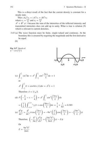
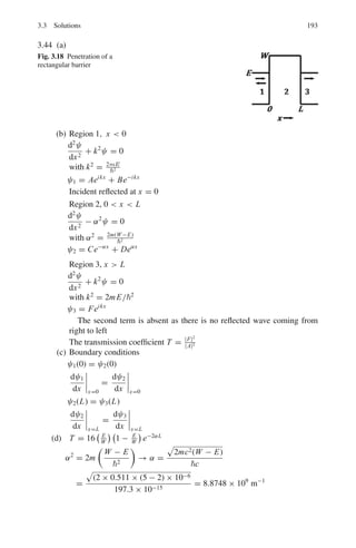
![158 3 Quantum Mechanics – II
This is the continuity equation where the probability current J = 1
2im
(ϕ∗
∇ϕ−
ϕ∇ϕ∗
)
And probability density
ρ =
i
2m
ϕ∗ ∂ϕ
∂t
− ϕ
∂ϕ∗
∂t
For a force free particle the solution of the Klein – Gordan equation is ϕ =
A ei(p.x−Et)
The probability density is
ρ =
i
2m
,
A∗
e−i(p.x−Et)
(i AE) e−i(p.x−Et)
−
Ae−i(p.x−Et)
i A∗
E
e−i(p.x−Et)
-
=
i
2m
,
A∗
A (−i E) − A A∗
(i E)
-
=
|A|2
2m
[E + E] = E
|A|2
m
As E can have positive and negative values, the probability density could
then be negative
3.6 (a) Class I: Refer to Problem 3.25
ψ1 = Aeβx
(−∞ x −a)
ψ2 = D cos αx (−a x +a)
ψ3 = Ae−βx
(a x ∞)
Normalization implies that
−a
−∞
|ψ1|2
dx +
a
−a
|ψ2|2
dx +
∞
a
|ψ3|2
dx = 1
−a
−∞
A2
e2βx
dx +
a
−a
D2
cos2
αxdx +
∞
a
A2
e−2βx
dx = 1
A2
e−2βa
/2β + D2
[a + sin(2αa)/2α] + A2
e−2βa
/2β = 1
Or
A2
e−2βa
/β + D2
(a + sin(2αa)/2α) = 1 (1)
Boundary condition at x = a gives
D cos α a = a e−βa
(2)
Combining (1) and (2) gives
D =
a +
1
β
−1
A = eβa
cosαa
a +
1
β
−1](https://image.slidesharecdn.com/1000-solved-problems-in-modern-physics-220626164600-18e7ea67/85/1000-solved-problems-in-modern-physics-pdf-212-320.jpg)
![3.3 Solutions 159
(b) The difference between the wave functions in the infinite and finite poten-
tial wells is that in the former the wave function within the well terminates
at the potential well, while in the latter it penetrates the well.
Fig. 3.4 Wave functions in potential wells of infinite and finite depths
3.7 Consider the expression
[x, [H, x]] =
2
μ
(1)
The expectation value in the initial state s is
s
%
%
%
%
2
μ
%
%
%
% s =
2
μ
s [x, Hx − x H] |s (2)
Using the wave function ψs and expanding the commutator
2
μ
= s
%
%2x Hx − x2
H − Hx2
%
% s (3)
Further s|x Hx|s =
k
s|x|k k|x|s Ek =
|xks|2
Ek (4)
where the summation is to be taken over all the excited states of the atom.
Also s|Hx2
|s = s|x2
H|s
=
k
s|x|k k|x|s Es =
|xks|2
Es (5)
Using (4) and (5) in (3) we get
2
/2μ =
k
|xks|2
(Ek − Es)
3.8 (a) The wave functions of the hydrogen atom, or for that matter of any atom,
with a central potential, are of the form
u(r) = λ(r)Pm
l (cos θ)eimϕ
Exchange of r → −r implies r → r, θ → π −θ and ϕ → π +ϕ (parity
operation)](https://image.slidesharecdn.com/1000-solved-problems-in-modern-physics-220626164600-18e7ea67/85/1000-solved-problems-in-modern-physics-pdf-213-320.jpg)
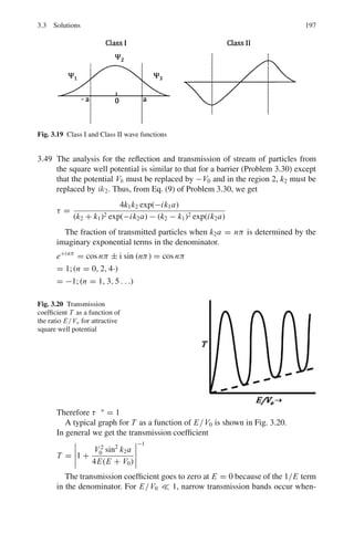
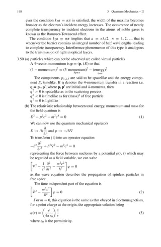
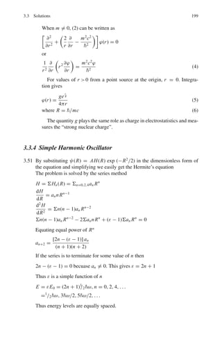
![3.3 Solutions 165
Integrating by parts twice
d
dt
Px = −
ψ∗
∂
∂x
(V ψ) − V
∂ψ
∂x
dτ
= −
ψ∗ ∂V
∂x
ψdτ =
−∂V
∂x
These two examples support the correspondence principle as they show
that the wave packet moves like a classical particle provided the expecta-
tion value gives a good representation of the classical variable.
3.15 (a) Using the Laplacian in the time-independent Schrodinger equation
−
2
2m
1
r2
∂
∂r
r2 ∂
∂r
+
1
r2 sin θ
∂
∂θ
sin θ
∂
∂θ
+
1
r2 sin2
θ
∂2
∂ϕ2
ψ(r, θ, ϕ) + V (r)ψ(r, θ, ϕ) = Eψ(r, θ, ϕ) (1)
We solve this equation by method of separation of variables
Let ψ (r, θ, ϕ) = ψr (r) Y(θ, ϕ) (2)
Use (2) in (1) and multiply by
−2m
2 .r2
/ψr (r)Y(θ, ϕ) and rearrange
1
ψr
(r)
d
dr
r2
dψr (r)/dr
+
2mr2
2
[E − V (r)]
= −
1
Y
(θ, ϕ)
1
sin θ
∂
∂θ
sin θ
∂
∂θ
(sin θ∂Y (θ, ϕ) /∂θ) +
1
sin2
θ
∂2
Y (θ, ϕ) /∂ϕ2
(3)
It is assumed that V (r) depends only on r.
L.H.S. is a function of r only and R.H.S is a function of θ and ϕ only.
Then each side must be equal to a constant, say λ.
1
sin θ
∂
∂θ
sin θ
∂Y
∂θ
θ, ϕ
+
1
sin2
θ
∂2
Y
∂ϕ2
θ, ϕ
+ λY (θ, ϕ) = 0 (4)
The radial equation is
d
dr
r2 dψr (r)
dr
+
2mr2
2
[E − V (r) − λ] ψr (r) = 0 (5)
(b) The angular equation (4) can be further separated by substituting
Y(θ, ϕ) = f (θ)g(θ) (6)](https://image.slidesharecdn.com/1000-solved-problems-in-modern-physics-220626164600-18e7ea67/85/1000-solved-problems-in-modern-physics-pdf-219-320.jpg)
![168 3 Quantum Mechanics – II
1
sin θ
∂
∂θ
sin θ
d f
dθ
+ λ f (θ) = 0 (2)
d
dθ
=
d
dμ
·
dμ
dθ
= − sin θ
d
dμ
Writing f (θ) = P(μ), Eq. (2) becomes
d
dμ
1 − μ2
dp
dμ
+ λP = 0
or
1 − μ2
d2
p
dμ2
− 2μ
dp
dμ
+ λp = 0 (3)
One can solve Eq. (3) by series method
Let P = Σ∞
k=1akμk
(4)
dp
dμ
=
k
akkμk−1
(5)
d2
P
dμ2
=
akk(k − 1)μk−2
(6)
Using (4), (5) and (6) in (3)
k(k − 1)akμk−2
−
k(k − 1)akμk
− 2
kakμk
+ λΣakμk
= 0
Equating equal powers of k
(k + 2)(k + 1)ak+2 − [k(k − 1) + 2k − λ] ak = 0
Or ak+2/ak = [k (k + 1) − λ] / (k + 1) (k + 2)
(b) If the infinite series is not terminated, it will diverge at μ = ±1, i.e. at
θ = 0 or θ = π. Because this should not happen the series needs to be
terminated which is possible only if λ = k(k + 1)
i.e. l(l + 1); l = 0, 1, 2 . . . Here l is known as the orbital angular momen-
tum quantum number. The resulting series P(μ) is then called Legendre
polynomial.
3.3.3 Potential Wells and Barriers
3.18 (a) The term − 2
d2
2mdx2 is the kinetic energy operator, U(x) is the potential
energy operator, ψ(x) is the eigen function and E is the eigen value.
(b) Put U(x) = 0 in the region 0 x a in the Schrodinger equation to
obtain
−
2
2m
d2
ψ(x)
dx2
= Eψ(x) (1)](https://image.slidesharecdn.com/1000-solved-problems-in-modern-physics-220626164600-18e7ea67/85/1000-solved-problems-in-modern-physics-pdf-222-320.jpg)
![170 3 Quantum Mechanics – II
a
0
ψ∗
n (x)ψn(x)dx = 1
A2
α
0
sin2
nπx
a
dx = 1
A2
2
x − cos
2nπx
a
%
%
%
a
0
= A2
a = 1
Therefore, A =
2
a
1/2
(9)
The normalized wave function is
ψn(x) =
2
a
1
2
sin
nπx
a
(10)
Using the value of α from (7) in (3), the energy is
En =
n2
h2
8ma2
(11)
(c) probability p =
a
0 |ψ3(x)|2
dx
=
2a
3
a
3
2
a
sin2
3πx
a
dx =
1
3
(d) ψ(n) and probability density P(x) distributions for n = 1, 2 and 3 are
sketched in Fig 3.6
Fig. 3.6
3.19 The Schrodinger equation for the n – p system in the CMS is
∇2
ψ(r, θ, ϕ) +
2μ
2
[E − V (r)]ψ(r, θ, ϕ) = 0 (1)](https://image.slidesharecdn.com/1000-solved-problems-in-modern-physics-220626164600-18e7ea67/85/1000-solved-problems-in-modern-physics-pdf-224-320.jpg)
![3.3 Solutions 171
Fig. 3.7 Deuteron wave
function and energy
where μ is the reduced mass = M/2, M, being neutron of proton mass. With
the assumption of spherical symmetry, the angular derivatives in the Laplacian
vanish and the radial equation is
1
r2
d
dr
r2 d
dr
ψ(r) + (M/2
)[E − V (r)]ψ(r) = 0 (2)
With the change of variable
ψ(r) =
u(r)
r
(3)
Equation (2) becomes
d2
u
dr2
+
M
2
[E − V (r)]u = 0 (4)
The total energy = −W, where W = binding energy, is positive as the poten-
tial is positive
V0 = −V , where V0 is positive
Equation (4) then becomes
d2
u
dr2
+
M
2
(V0 − W) u = 0; r R (5)
d2
u
dr2
−
MWu
2
= 0; r R (6)
where R is the range of nuclear forces, Fig. 3.7.
Calling
M(V0 − W)
2
= k2
(7)
and
MW
2
= γ 2
(8)
(5) and (6) become
d2
u
dr2
+ k2
u = 0 (9)
d2
u
dr2
− γ 2
u = 0 (10)](https://image.slidesharecdn.com/1000-solved-problems-in-modern-physics-220626164600-18e7ea67/85/1000-solved-problems-in-modern-physics-pdf-225-320.jpg)
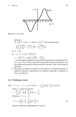
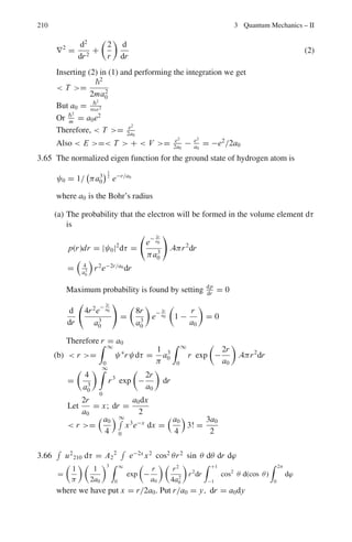
![174 3 Quantum Mechanics – II
The ground state corresponds to n = 1 and the first excited state to n =
2, m = 8me and L = 1 nm = 106
fm. Putting n = 1 in (3)
hv = E2 − E1 =
3h2
8mL2
= 3π2
2
c2
/16mec2
L2
= 3π2
(197.3)2
MeV2
− fm2
/(16 × 0.511 MeV)(106
)2
fm2
= 0.14 × 10⁻⁶
MeV = 0.14 eV
λ(nm) =
1,241
E(eV)
=
1,241
0.14
= 8864 nm
This corresponds to the microwave region of the electro-magnetic spectrum.
3.25 Consider a finite potential well. Take the origin at the centre of the well.
V (x) = V0; |x| a
= 0; |x| a
d2
ψ
dx2
+
2m
2
[E − V (r)] ψ = 0
Region 1 (E V0)
d2
ψ
dx2
−
2m
2
(V0 − E)ψ = 0 (1)
d2
ψ
dx2
− β2
ψ = 0 (2)
where β2
=
2m
2
(V0 − E) (3)
ψ1 = Aeβx
+ Be−βx
(4)
where A and B are constants of integration.
Since x is negative in region 1, and ψ1 has to remain finite we must set B = 0,
otherwise the wave function grows exponentially. The physically accepted
solution is
ψ1 = Aeβx
(5)
Region 2; (V = 0)
Fig. 3.8 Square potential
well of finite depth](https://image.slidesharecdn.com/1000-solved-problems-in-modern-physics-220626164600-18e7ea67/85/1000-solved-problems-in-modern-physics-pdf-228-320.jpg)
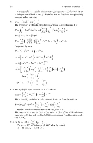
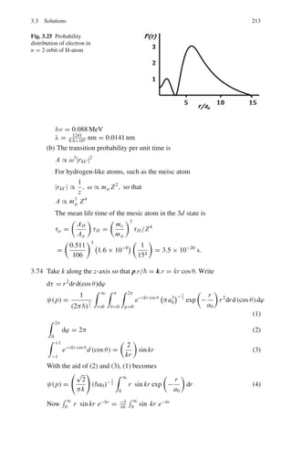
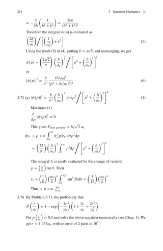
![178 3 Quantum Mechanics – II
R
0
|ψ1|2
dτ +
∞
R
|ψ2|2
dτ = 1
R
0
u2
1.4πr2
dr/r2
+
∞
R
u2
24πr2
dr/r2
= 1
A2
R
0
sin2
krdr + C2
∞
R
e−2γ r
dr = 1/4π
Integrating and using (2), we find
A2
=
γ
2π(γR + 1)
(4)
Using (4) in (3)
P =
1
γ R + 1
(5)
Now γ R =
MW
2
1/2
R =
Mc2
W
2c2
1/2
R
=
940 × 2.2
(197.3)2
1/2
× 2.1 = 0.48
where we have inserted Mc2
= 940 MeV /c2
,
W = 2.2MeV and R = 2.1 f m
Therefore p = 1
0.48+1
= 0.67
Thus neutron and proton stay outside the range of nuclear forces approxi-
mately 70% of time.
3.27 By Problem 3.25, for the finite well, for class I
α tan αa = β
with α =
(2mE)
1
2
; β =
[2m(V0 − E)]
1
2
As V0 → ∞, β → ∞ and αa = nπ/2 (n odd)
Therefore, α2
a2
= 2mEa2
2 = n2
π2
4
Or E = n2
π2
2
/8ma2
(n odd)
For class II
α cot αa = −β
As V0 → ∞, β → ∞ and αa = nπ/2 (n even)](https://image.slidesharecdn.com/1000-solved-problems-in-modern-physics-220626164600-18e7ea67/85/1000-solved-problems-in-modern-physics-pdf-232-320.jpg)
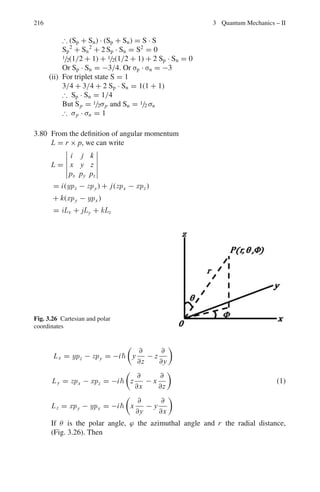
![3.3 Solutions 199
When m
= 0, (2) can be written as
∂2
∂r2
+
2
r
∂
∂r
−
m2
c2
2
ϕ(r) = 0
or
1
r2
∂
∂r
r2 ∂ϕ
∂r
=
m2
c2
ϕ
2
(4)
For values of r 0 from a point source at the origin, r = 0. Integra-
tion gives
ϕ(r) =
ge
r
R
4πr
(5)
where R = /mc (6)
The quantity g plays the same role as charge in electrostatistics and mea-
sures the “strong nuclear charge”.
3.3.4 Simple Harmonic Oscillator
3.51 By substituting ψ(R) = AH(R) exp (−R2
/2) in the dimensionless form of
the equation and simplifying we easily get the Hermite’s equation
The problem is solved by the series method
H = ΣHn(R) = Σn=0,2,4an Rn
dH
dR
= annRn−1
d2
H
dR2
= Σn(n − 1)an Rn−2
Σn(n − 1)an Rn−2
− 2ΣannRn
+ (ε − 1)Σan Rn
= 0
Equating equal power of Rn
an+2 =
[2n − (ε − 1)] an
(n + 1)(n + 2)
If the series is to terminate for some value of n then
2n − (ε − 1) = 0 becuase an
= 0. This gives ε = 2n + 1
Thus ε is a simple function of n
E = εE0 = (2n + 1)1
/2ω, n = 0, 2, 4, . . .
=1
/2ω, 3ω/2, 5ω/2, . . .
Thus energy levels are equally spaced.](https://image.slidesharecdn.com/1000-solved-problems-in-modern-physics-220626164600-18e7ea67/85/1000-solved-problems-in-modern-physics-pdf-264-320.jpg)
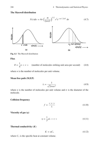
![m
k
n +
1
2
=
n +
1
2
Thus, Δx.ΔP ≥
2
is in agreement with uncertainty principle.
3.59 The vibrational levels are equally spaced and so with the rule Δn = 1, the lines
should coincide. The rotational levels are progressively further spaced such
that the difference in the wave number of consecutive lines must be constant.
This can be seen as follows:
EJ =
J(J + 1)2
2I0
c
λJ
= ΔE = EJ+1 − EJ =
[(J + 1) (J + 2) − J(J + 1)] 2
2I0
=
(J + 1)2
2I0
Therefore 1
λJ+1
− 1
λJ
= Δ
1
λJ
α[(J + 2) − (J + 1)] = constant
103.73 − 83.03 = 20.70 cm−1
; 124.30 − 103.73 = 20.57 cm−1
;
145.03 − 124.30 = 20.73 cm−1
; 165.51 − 145.03
= 20.48 cm−1
; 185.86 − 165.51 = 20.35 cm−1
The data are consistent with a constant difference, the mean value being,
20.556 cm−1
. Thus the transitions are rotational.
EJ+1 EJ
EJ+2 − EJ+1
=
2(J + 1)
2(J + 2)
=
83.03
103.73
= 0.8
Therefore J = 3
The levels are characterized by J = 3, 4, 5, 6, 7, 8, 9](https://image.slidesharecdn.com/1000-solved-problems-in-modern-physics-220626164600-18e7ea67/85/1000-solved-problems-in-modern-physics-pdf-274-320.jpg)
![3.3 Solutions 207
c
1
λj+1
−
1
λj
= c × (20.556 cm−1
) =
2
I0
Moment of inertia I0 =
4π2c × 20.556
=
6.63 × 10⁻²⁷
erg − s−1
4π2 × 3 × 1010 cm − s−1 × 20.556 cm−1
= 2.727 × 10−40
g − cm2
I0 = μr2
μ =
m(H)m(Cl)
[m(H) + m(Cl)]
=
1 × 35 × 1.67
1 + 35
× 10−24
g
= 1.62 × 10⁻²⁴
g
r =
I0
μ
1/2
=
2.727 × 10−40
1.62 × 10−24
= 1.3 × 10⁻⁸
cm = 1.3 Å
3.60 For the 3-D isotropic oscillator the energy levels are given by
EN = Ek + El + Em =
3
2
+ nk + nl + nm
ω
where ω is the angular frequency
N = nk + nl + nm = 0, 1, 2 . . .
For a given value of N, various possible combinations of nk, nl and nm are
given in Table 3.5, and the degeneracy indicated.
Table 3.5 Possible combinations of nk, nl and nm and degeneracy of energy levels
N nl nm nn Degeneracy (D)
0 0 0 0 Non-degenerate
1 1 0 0 Three fold (1 + 2)
0 1 0
0 0 1
2 1 1 0 Sixfold (1 + 2 + 3)
1 0 1
0 1 1
2 0 0
0 2 0
0 0 2
3 1 1 1 Tenfold (1 + 2 + 3 + 4)
1 2 0
1 0 2
2 1 0
2 0 1
0 2 1
0 1 2
3 0 0
0 3 0
0 0 3](https://image.slidesharecdn.com/1000-solved-problems-in-modern-physics-220626164600-18e7ea67/85/1000-solved-problems-in-modern-physics-pdf-275-320.jpg)
![208 3 Quantum Mechanics – II
It is seen from the last column of the table that the degeneracy D is given by
the sum of natural numbers, that is, = n(n + 1)/2, if we replace n by N + 1,
D = (N + 1)(N + 2)/2.
3.61 As the time evolves, the eigen function would be
ψ(x, t) =
n=0.1 Cnψn(x) exp(−i Ent/)
= C0ψ0(x) exp(−i E0t/) + C1ψ1(x) exp(−i E1t/)
The probability density
|ψ(x, t)|2
= C2
0 + C2
1 + C0C1ψ0(x)ψ1(x)[exp(i(E1 − E0)t/)
− exp(−i(E1 − E0)t/)]
= C2
0 + C2
1 + 2C0C1ψ0(x)ψ1(x) cos ω t
where we have used the energy difference E1 − E0 = ω. Thus the probability
density varies with the angular frequency.
3.62 E =
n=1,2,3
|Cn|2
En = C2
0 E0 + C2
1 E1 + C2
2 E2
=
1
2
·
ω
2
+
1
3
·
3ω
2
+
1
6
·
5ω
2
=
7ω
6
.
3.63 (a) ψ0(x) = A exp(−x2
/2a2
)
Differentiate twice and multiply by −2
/2m
−
2
2m
d2
ψ0
dx2
=
A2
2ma2
1 −
x2
a2
exp
−
x2
2a2
=
2
2ma2
ψ0 −
2
x2
2ma4
ψ0
or −
2
2m
d2
ψ0
dx2
+
2
x2
2ma4
ψ0 =
2
2ma2
ψ0
Compare the equation with the Schrodinger equation
E =
2
2ma2
=
ω
2
ω =
ma2
(1)
or a =
mω
1/2
Same relation is obtained by setting
V =
2
x2
2ma4
=
mω2
x2
2
(b) ψ1 = Bx exp
− x2
2a2
Differentiate twice and multiply by − 2
2m
−
2
2m
d2
ψ1
dx2
=
B2
x3
exp
x2
a
2ma4
+
3B2
exp
− x2
2a2
2ma2](https://image.slidesharecdn.com/1000-solved-problems-in-modern-physics-220626164600-18e7ea67/85/1000-solved-problems-in-modern-physics-pdf-276-320.jpg)
![212 3 Quantum Mechanics – II
Writing sin2
θ = 1−cos2
θ and simplifying we get u∗
u = 2
9
A2
3e−2x
x4
which
is independent of both θ and ϕ. Therefore the 3d functions are spherically
symmetrical or isotropic.
3.71 ψ100 =
πa3
0
− 1
2
exp
− r
a0
The probability p of finding the electron within a sphere of radius R is
P =
R
0
|ψ100|2
.4πr2
dr =
4π
πa3
0
R
0
r2
exp
−
2r
a0
dr
Set 2r
a0
= x; dr =
a0
2
dx
P =
4
a3
0
·
a2
0
4
·
a0
2
x2
e−x
dx = 1
/2
x2
e−x
dx
Integrating by parts
P = 1
/2[−x2
e−x
+ 2
xe−x
dx]
= 1
/2
−x2
e−x
+ 2
−x e−x
+
e−x
dx
= 1
/2
,
−x2
e−x
− 2xe−x
− 2e−x
-2R/a0
0
= 1
/2
−
2R
a0
2
exp
−
2R
a0
− 2
2R
a0
exp
−
2R
a0
−2 exp
−
2R
a0
+ 2
P = 1 − e
− 2R
a0
1 +
2R
a0
+
2R2
a2
0
3.72 The hydrogen wave function for n = 2 orbit is
ψ200 =
1
4
2πa3
0
− 1
2
2 −
r
a0
e−r/2a0
The probability of finding the electron at a distance r from the nucleus
P = |ψ200|2
· 4πr2
=
1
8
r2
a3
0
2 −
r
a0
2
exp
−
r
a0
Maxima are obtained from the condition dp/dr = 0.
The maxima occur at r = (3 −
√
3)a0 and r = (3 +
√
3)a0 while minimum
occur at r = 0, 2a0 and ∞ (Fig. 3.25) (the minima are found from the condi-
tion p = 0).
3.73 (a) hν = 13.6 Z2
mμ
me
1
22 − 1
32
Put mμ = 106 MeV (instead of 106.7 MeV for muon)
Z = 15 and me = 0.511 MeV](https://image.slidesharecdn.com/1000-solved-problems-in-modern-physics-220626164600-18e7ea67/85/1000-solved-problems-in-modern-physics-pdf-280-320.jpg)
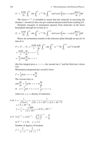
![214 3 Quantum Mechanics – II
= −
∂
∂b
k
b2 + k2
=
2kb
(b2 + k2)2
Therefore the integral in (4) is evaluated as
2k
a0
3
1
a2
0
+ k2
(5)
Using the result (5) in (4), putting k = p/, and rearranging, we get
ψ(p) =
2
√
2
π
#
a0
5
2
4
p2
+
a0
2
'2
or
|ψ(p)|2
=
8
π2
(/a0)5
[p2 + (/a0)2
]4
(6)
3.75 (a) |ψ(p)|2
=
8
π2
a0
5
.4 πp2
4
p2
+
a0
2
'4
(1)
Maximize (1)
d
dp
|ψ(p)|2
= 0
This gives Pmost probable = /
√
3 a0
(b) p =
∞
0
ψ∗
p pψp.4πp2
dp
=
32
π
a0
5 ∞
0
p3
dp
4
p2
+
a0
2
'4
The integral I1 is easily evaluated by the change of variable
p =
a0
tan θ. Then
I1 =
1
8
a0
4
π/2
0
sin3
2θdθ =
1
12
a0
4
Thus p = 8
3πa0
3.76 By Problem 3.71, the probability that
P
r
a0
= 1 − exp
−
2r
a0
1 +
2r
a0
+
2r2
a2
0
Put p
r
a0
= 0.5 and solve the above equation numerically (see Chap. 1). We
get r = 1.337a0, with an error of 2 parts in 105
.](https://image.slidesharecdn.com/1000-solved-problems-in-modern-physics-220626164600-18e7ea67/85/1000-solved-problems-in-modern-physics-pdf-282-320.jpg)
![3.3 Solutions 215
3.3.6 Angular Momentum
3.77 L =
%
%
%
%
%
%
i j k
x y z
px py pz
%
%
%
%
%
%
= i(ypz − zpy) − j(xpz − zpx ) + k(xpy − ypx )
= i Lx + j Ly + kLz
Thus, Lx = ypz − zpy, Ly = zpx − xpz, Lz = xpy − ypx (1)
[Lx , Ly] = Lx Ly − Ly Lx
= (ypz − zpy)(zpx − xpz) − (zpx − xpz)(ypz − zpy)
= ypz zpx − ypz xpz − zpyzpx + zpy xpz − zpx ypz + zpx zpy
+ xpz ypz − xpzzpy (2)
But [px , py] = [x, py] = 0, etc (3)
(2) becomes
[Lx , Ly] = ypx pzz − yxp2
z − z2
py px + xpyzpy − ypx zpz + z2
px py
+ yxp2
z − xpy pz z = [z, pz](xpy − ypz) (4)
But [z, pz] = [z, −i
∂
∂z
] = −i
z,
∂
∂z
(5)
Further,
z,
∂
∂z
= −1 (6)
So
[z, pz ] = i (7)
Combining (1), (4) and (7) we get
[Lx , Ly] = iLz (8)
3.78 Given spin state is a singlet state, that is S = 0
S1 + S2 = S
Form scalar product by itself
S1 · S1 + S1 · S2 + S2 · S1 + S2 · S2 = S · S
S1
2
+ 2 S1 · S2 + S2
2
= S2
= 0
Now, S1
2
= S2
2
= (1/2)(1/2 + 1) = 3/4
Therefore S1 · S2 = −(3/4) 2
3.79 For the n – p system
Sp + Sn = S
and Sp
2
= Sn
2
= s(s + 1) with s = 1/2
(i) For singlet state, S = 0](https://image.slidesharecdn.com/1000-solved-problems-in-modern-physics-220626164600-18e7ea67/85/1000-solved-problems-in-modern-physics-pdf-283-320.jpg)
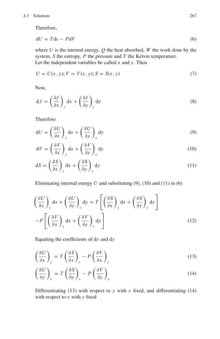
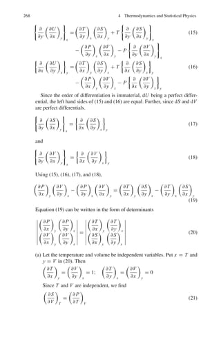
![218 3 Quantum Mechanics – II
Now Lz g(ϕ) = −i∂g
∂ϕ
= mg(ϕ)
Thus the z-component of angular momentum is quantized with eigen
value .
3.81 One can do similar calculations for Lx and Ly as in Problem 3.80 and obtain
Lx
i
= sin ϕ
∂
∂θ
+ cot θ cos ϕ
∂
∂ϕ
Ly
i
= − cos ϕ
∂
∂θ
+ cot θ sin ϕ
∂
∂ϕ
3.82 Using L2
= L2
x + L2
y + L2
z , the commutator with total angular momentum
squared can be evaluated
[L2
, Lz] =
,
L2
x + L2
y + L2
z , Lz
-
=
,
L2
x + L2
y, Lz
-
= Lx [Lx , Lz] + [Lx , Lz] Lx + Ly
,
Ly, Lz
-
+
,
Ly, Lz
-
Ly (1)
= −iLx Ly − iLy Lx + iLy Lx + iLx Ly = 0
Similarly
,
L2
, Lx
-
= [L2
, Ly] = [L2
, L] = 0
3.83 L2
= L2
x + L2
y + L2
z
Using the expressions for Lx , Ly and Lz from problem (3.81)
L2
(i)2
=
sin ϕ
∂
∂θ
+ cot θ cos ϕ
∂
∂ϕ
sin ϕ
∂
∂θ
+ cot θ cos ϕ
∂
∂ϕ
+
− cos ϕ
∂
∂θ
+ cot θ sin ϕ
∂
∂ϕ
− cos ϕ
∂
∂θ
+ cot θ sin ϕ
∂
∂ϕ
+
−
∂
∂ϕ
−
∂
∂ϕ
= sin2
ϕ
∂2
∂θ2
+ cot2
θ cos2
ϕ
∂2
∂ϕ2
− sin ϕ cos ϕ cosec2
θ
∂
∂ϕ
+ cos2
ϕ cot θ
∂
∂θ
+ cos2
ϕ
∂2
∂θ2
+ cot2
θ sin2
ϕ
∂2
∂ϕ2
+ sin ϕ cos ϕcosec2
θ
∂
∂ϕ
+ sin2
ϕ cot θ
∂
∂θ
+
∂2
∂ϕ2
The cross terms get cancelled and the expression is reduced to
∂2
∂θ2
+
1
sin2
θ
∂2
∂ϕ2
+ cot θ
∂
∂θ
∇2
ψ =
1
r2
∂
∂r
r2 ∂ψ
∂r
+
1
r2 sin θ
∂
∂θ
sin θ
∂ψ
∂θ
+
1
r2 sin2
θ
∂2
ψ
∂ϕ2](https://image.slidesharecdn.com/1000-solved-problems-in-modern-physics-220626164600-18e7ea67/85/1000-solved-problems-in-modern-physics-pdf-286-320.jpg)
![3.3 Solutions 219
Apart from the factor 1/r2
, the angular part is seen to be
∂2
ψ
∂θ2
+ cot θ
∂ψ
∂θ
+
1
sin2
∂2
ψ
∂ϕ2
3.84 (a) The (i, j)th matrix element of an operator O is defined by
Oij = i|o| j (1)
For j = 1/2, m = 1/2 and −1/2. The two states are
|1 = |
1
2
,
1
2
and |2 = |
1
2
, −
1
2
(2)
With the notation | j, m
Now
j
m
|Jz|jm = mδjj δmm (3)
Thus
(Jz)11 = 1|Jz|1 =
1
2
(4)
(Jz)22 = 2|Jz|2 = −
1
2
(5)
(Jz)12 = 1|Jz|2 =
5
1
2
,
1
2
|Jz|
1
2
,
1
2
6
= 0 (6)
because of (3).
Similarly
(Jz)21 = 0 (7)
Therefore
Jz =
2
1 0
0 −1
(8)
For Jx and Jy, we use the relations
Jx = 1
/2(J+ + J−) and Jy = −
1
2i
(J+ − J−)
j, m|Jx | j, m = j, m|
1
2
(J+ + J−)| j, m
= 1
/2[( j + m + 1)( j − m)]1/2
j, m
| j, m + 1
+ 1
/2[( j − m + 1)( j + m)]1/2
j, m
| j, m − 1
= 1
/2[( j + m + 1)( j − m)]1/2
δm ,m+1
+ 1
/2[( j − m + 1)( j + m)]
1
/2
δm ,m−1
That is the matrix element is zero unless m
= m + 1 or m
= m − 1.
The first delta factor survives](https://image.slidesharecdn.com/1000-solved-problems-in-modern-physics-220626164600-18e7ea67/85/1000-solved-problems-in-modern-physics-pdf-287-320.jpg)
![220 3 Quantum Mechanics – II
(Jx )12 = 1|Jx |2 =
5
1
2
,
1
2
|Jx |
1
2
, −
1
2
6
=
1
2
1
2
−
1
2
+ 1
1
2
+
1
2
1/2
= 1
/2
(Jx )21 =
5
1
2
, −
1
2
|J|
1
2
,
1
2
6
= 1
/2
because the second delta factor survives
(Jx )11 = 1|Jx |1 =
71
2
, 1
2
|Jx |1
2
, 1
2
8
= 0 because of delta factors.
Similarly, (Jx )22 = 0
Thus Jx =
2
0 1
1 0
; Jy =
2
0 −i
i 0
Jz =
2
1 0
0 −1
(9)
These three matrices are known as Pauli matrices.
(b) J2
= J2
x + J2
y + J2
z
Using the matrices given in (6), squaring them and adding we get
J2
= 3
/42
1 0
0 1
3.85 (a) For j = 1, m = 1, 0 and −1, the three base states are denoted by
|1 , |2 and |3 . In the | j, m notation |1 = |1, 1 , |2 =
|1, 0 , |3 = |1, −1
Jz|1 = m|1 = |1
Jz|2 = 0.|2 = 0
Jz|3 = −|3
(Jz)11 = 1|Jz|1 = 1, 1|Jz|1, 1 =
(Jz)22 = 2|Jz|2 = 1, 0|Jz|1, 0 = 0
(Jz)33 = 3|Jz|3 = 1, −1|Jz|1, −1 = −
(Jz)12 = (Jz)21 = (Jz)13 = (Jz)31 = (Jz)23 = (Jz)32 = 0
because of δ – factor δmm
Jz =
⎛
⎝
1 0 0
0 0 0
0 0 −1
⎞
⎠
For the calculation of Jx and Jy, we need to work out J+ and J−.
J+|1 = 0
J+|2 = [( j − m)( j + m + 1)]1/2
|1](https://image.slidesharecdn.com/1000-solved-problems-in-modern-physics-220626164600-18e7ea67/85/1000-solved-problems-in-modern-physics-pdf-288-320.jpg)
![3.3 Solutions 221
= [(1 − 0)(1 + 0 + 1)]1/2
|1 =
√
2|1
J+
%
%
%3 = [[1 − (−1)](1 − 1 + 1)]
1
2
%
%
% 2 =
√
2 |2
J−|1 = [( j + m)( j − m + 1)]1/2
|2
= [(1 + 1)(1 − 1 + 1)]1/2
|2 =
√
2 |2
J−|2 =
√
2 |3
J−|3 = 0
Matrices for Jx and Jy:
(Jx )11 = 1|Jx |1 = 1
/2 1|J+ + J−|1
= 1
/2 1|J+|1 +
1
2
1|J−|1
= 1
/2[( j − m)( j + m + 1)]1/2
δm m+1
+ 1
/2[( j + m)( j − m + 1)]1/2
δm ,m−1=0
Similarly; (Jx )22 = (Jx )33 = 0
(Jx )12 = 1|Jx |2 = 1/2 1|J+ + J−|2 = 1/2 1, 1|J+ + J−|1, 0
= 1
/2[( j − m)( j + m + 1)]1/2
δm m+1 + 1/2[( j + m)( j − m + 1)]1/2
δm m−1
The second delta is zero
∴ (Jx )12 =
1
2
[(1 + 0)(1 + 0 + 1)]1/2
=
√
2
Similarly, (Jx )21 = (Jx )23 = (Jx )32 =
√
2
By a similar procedure the matrix elements of Jy can be found out. Thus
Jx =
√
2
⎛
⎝
0 1 0
1 0 1
0 1 0
⎞
⎠ ; Jy =
√
2
⎛
⎝
0 −i 0
i 0 −i
0 i 0
⎞
⎠ ; Jz =
⎛
⎝
1 0 0
0 0 0
0 0 −1
⎞
⎠
(b) For the matrix elements of J we can use the relation
j
m
|J2
|jm = j( j + 1)2
δj j δm m
Thus (J2
)11 = (J2
)22 = (J2
)33 = 1(1 + 1)2
= 22
(J2
)12 = (J2
)21 = (J2
)13 = (J2
)31 = (J2
)23 = (J2
)32 = 0
J2
= 22
⎛
⎝
1 0 0
0 1 0
0 0 1
⎞
⎠
Alternatively, J2
= J2
x + J2
y + J2
z
Using the matrices which have been derived the same result is obtained.
3.86 With the addition of j1 = 1 and j2 = 1/2, one can get J = 3/2 or 1/2. In the
(J, M) notation in all one gets 6 states
ψ
3
2
,
3
2
, ψ
3
2
,
1
2
, ψ
3
2
, −
1
2
, ψ
3
2
, −
3
2
and ψ
1
2
,
1
2
, ψ
1
2
, −
1
2](https://image.slidesharecdn.com/1000-solved-problems-in-modern-physics-220626164600-18e7ea67/85/1000-solved-problems-in-modern-physics-pdf-289-320.jpg)
![222 3 Quantum Mechanics – II
Clearly the states ψ
3
2
, 3
2
and ψ
3
2
, −3
2
can be formed in only one way
ψ
3
2
,
3
2
= ϕ(1, 1)ϕ
1
2
,
1
2
(1)
ψ
3
2
, −
3
2
= ϕ(1, −1)ϕ
1
2
, −
1
2
(2)
We now use the ladder operators J+ and J− to generate the second and the
third states.
J+ϕ( j, m) = [( j − m)( j + m + 1)]
1
2 ϕ( j, m + 1) (3)
J−ϕ( j, m) = [( j + m)( j − m + 1)]
1
2 ϕ( j, m − 1) (4)
Applying (4) to (1) on both sides
J−ψ
3
2
,
3
2
=
3
2
+
3
2
3
2
−
3
2
+ 1
1/2
=
√
3ψ
3
2
,
1
2
= J−ϕ(1, 1)ϕ
1
2
,
1
2
= ϕ(1, 1)J−
1
2
,
1
2
+ ϕ
1
2
,
1
2
J−ϕ(1, 1)
= ϕ(1, 1)ϕ
1
2
, −
1
2
+ ϕ
1
2
,
1
2
√
2ϕ(1, 0)
Thus ψ
3
2
,
1
2
=](https://image.slidesharecdn.com/1000-solved-problems-in-modern-physics-220626164600-18e7ea67/85/1000-solved-problems-in-modern-physics-pdf-290-320.jpg)
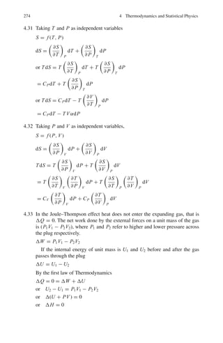
![2
3
ϕ(1, −1)ϕ
1
2
,
1
2
(12)
The coefficients appearing in (1), (2), (5), (6), (11) and (12) are known as
Clebsch – Gordon coefficients. These are displayed in Table 3.3.
3.87 In spherical coordinates
x = r sin θ cos ϕ ; y = r sin θ sin ϕ ; z = r cos θ (1)
So that xy + yz + zx = r2
sin2
θ sin ϕ cos ϕ + r2
sin θ cos θ sin ϕ
+ r2
sin θ cos θ cos ϕ (2)
The spherical harmonics are
Y00 =
1
4π
1/2
; Y10 =
3
4π
1/2
cos θ ; Y1±1 = ∓
3
8π
1/2
sin θ e±ϕ
Y20 =
5
16π
1
2
(3 cos2
θ − 1); Y2±1 = ∓
15
8π
1
2
sin θ cos θ e±iϕ
;
Y2±2 =
15
32π
1/2
sin2
θ e±2iϕ
(3)
Expressing (2) in terms of (3),
sin2
θ sin ϕ cos ϕ = 1
/2 sin2
θ sin 2ϕ =
Y22 − Y2−2
4i
32π
15
1/2
Similarly sin θ cos θ sin ϕ =
8π
15
1/2 (Y21−Y2−1)
2i
sin θ cos θ cos ϕ =
8π
15
1
2
(Y21 − Y2−1)/2
Hence, xy + yz + zx = r2
8π
15
1
2
[(Y22 − Y2−1)/i + (Y21 + Y2−1)/2i
+(Y21 − Y2−1)/2]
The above expression does not contain Y00 corresponding to l = 0, nor
Y10 and Y1±1 corresponding to l = 1. All the terms belong to l = 2, and the
probability for finding l = 2 and therefore L2
= l(l + 1) = 62
is unity.
3.88 Lz = −i
∂
∂ϕ
x = r sin θ cos ϕ ; y = r sin θ sin ϕ ; z = r cos θ
ψ1 = (x + iy) f (r) = r sin θ(cos ϕ + i sin ϕ) f (r)
= (cos ϕ + i sin ϕ) sin θ F(r)](https://image.slidesharecdn.com/1000-solved-problems-in-modern-physics-220626164600-18e7ea67/85/1000-solved-problems-in-modern-physics-pdf-303-320.jpg)
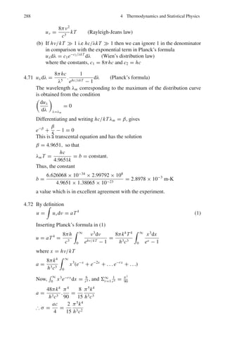
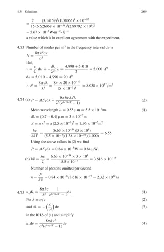
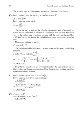
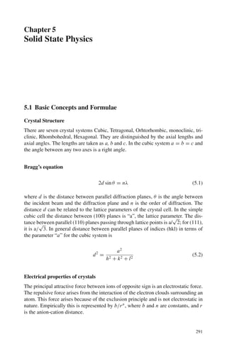
![15
32π
sin2
θ(e2iϕ
+ e−2iϕ
) (4)
Dividing (1) by (4) and simplifying we get
u(θ, ϕ) =
1
√
2
(Y2+2(θ, ϕ) + Y2−2(θ, ϕ))
We know that
L2
Ylm = 2
l(l + 1)Ylm
So L2
u(θ, ϕ) = L2
[Y22(θ,ϕ)+Y2−2(θ,ϕ)]
√
2
= 2(2 + 1)2 [Y22(θ,ϕ)+Y2−2(θ,ϕ)]
√
2
= 62
u(θ, ϕ)
Thus the eigen value of L2
is 62
3.94 The wave function is identified as ψ322
LZ ψ = −i
∂ψ
∂ϕ
= 2ψ
Thus the eigen value of LZ is 2.
3.95 (a) Using the values, Y10 =
$
3
4π
cos θ and Y1,±1 = ∓
$
3
8π
sin θ exp(±iϕ), we
can write
ψ =](https://image.slidesharecdn.com/1000-solved-problems-in-modern-physics-220626164600-18e7ea67/85/1000-solved-problems-in-modern-physics-pdf-312-320.jpg)
![1
3
Y10
'2
dΩ =
+1
−1
3
4π
.2π cos2
θd cos θ = 1/3
3.96 (a) [Jz, J+] = Jz J+ − J+ Jz = Jz(Jx + iJ y) − (Jx + iJ y)Jz
= Jz Jx − Jx Jz + i(Jz Jy − Jy Jz)
= [Jz, Jx ] + i[Jz, Jy] = iJy − iiJx
= iJy + Jx = (Jx + iJ y) = J+
= J+, in units of .
(b) From (a), Jz J+ = J+ Jz + J+
Jz J+|j m = J+ Jz|jm +J+|jm
= J+m|jm +J+|jm
= (m + 1)J+|jm
J+|jm is nothing but | j, m + 1 apart from a possible normalization
constant. Thus
J+|jm = Cjm+ | j, m + 1
Given a state |jm , the state | j, m + 1 must exist unless Cjm+ van-
ishes for that particular m. Since j is the maximum value of m by definition.
There can not be a state | j, j + 1 , i.e. Cjj+ must vanish. J+ is known as
the ladder operator. Similarly, J− lowers m by one unit.
(c) J+ = Jx + iJ y
J− = Jx − iJ y
Therefore, Jx =
1
2
(J+ + J−) =
⎛
⎝
0 1/
√
2 0
1/
√
2 0 1/
√
2
0 1/
√
2 0
⎞
⎠
Jy =
1
2i
(J+ − J−) =
⎛
⎝
0 −i/
√
2 0
i/
√
2 0 −i/
√
2
0 i/
√
2 0
⎞
⎠
[Jx , Jy] = Jx Jy − Jy Jx = i
⎛
⎝
1 0 0
0 0 0
0 0 −1
⎞
⎠ = iJ z](https://image.slidesharecdn.com/1000-solved-problems-in-modern-physics-220626164600-18e7ea67/85/1000-solved-problems-in-modern-physics-pdf-316-320.jpg)
![230 3 Quantum Mechanics – II
= 1
/2 m ω2
[(x + qE/mω2
)2
− q2
E2
/m2
ω4
]
= 1
/2 mω2
x +
qE
mω2
2
−
q2
E2
2mω2
(2)
Put X = x + qE
mω2 ; then we can write
d
dx
=
d
dX
and
d2
dx2
=
d2
dX2
Equation (1) becomes
−
2
2m
d2
dX2
+
1
2
mω2
X2
ψn(X) =
En +
q2
E2
2mω2
ψn(X) (3)
Left hand side of (3) is the familiar Hamiltonian for the Simple harmonic
oscillator. The modified eigen values are then given by the right hand side
En +
q2
E2
2mω2
=
n +
1
2
ω
or
En =
n +
1
2
ω − q2
E2
/2mω2
(4)
3.99 The matrix of H
is
(H
) =
H
11 H
12
H
21 H
22
, with H
12 = H ∗
21
The matrix of H is
H =
E0 + H
11 H
12
H
21 E0 + H
22
%
%
%
%
E0 + H
11 − E H
12
H
21 E0 + H
22 − E
%
%
%
% = 0
E1 = 1
/2
2E0 + H
11 + H
22
+ 1
/2
*
H
11 − H
22
2
+ 4
%
%H
12
%
%2
+1/2
E2 = 1
/2
2E0 + H
11 + H
22
− 1
/2
*
H
11 − H
22
2
+ 4
%
%H
12
%
%2
+1/2
These are the energy levels of a two state system with Hamiltonian H =
H0 + H
. The perturbation theory requires finding the eigen values of H
and
adding them to E0, which gives an exact result.
3.100 The nuclear charge seen by the electron is Z and not 2. This is because of
screening the effective charge is reduced.
The smallest value of E(Z) = − e2
2a0
27
4
Z − 2Z2
must be determined
which is done by setting](https://image.slidesharecdn.com/1000-solved-problems-in-modern-physics-220626164600-18e7ea67/85/1000-solved-problems-in-modern-physics-pdf-318-320.jpg)
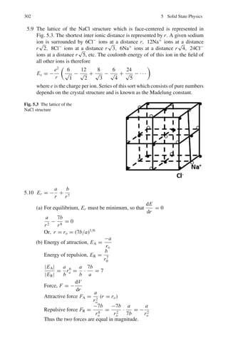
![3.3 Solutions 235
or eikr
f (θ) =
Bl pl(cos θ)
*
ei(kr− πl
2
+δl ) − e−i(kr− πl
2
+δl )
+
2ik
−
il
(2l + 1)pl(cos θ)
*
ei(kr− πl
2 ) − e−i(kr− πl
2 )
+
2ik
Equating coefficients of e−ikr
0 = −
1
2ik
Bl pl (cos θ)
e−i(−πl/2+δl )
+
il
(2l + 1)Pl(cos θ)
2ik
eiπl/2
Therefore
Bl = il
(2l + 1)eiδl
(12)
Equating coefficients of eikr
, and using the value of Bl
f (θ) =
1
2ik
*
il
(2l + 1)eiδl
pl(cos θ)ei(− πl
2
+δl )
−
il
(2l + 1)pl (cos θ)e− πl
2
+
=
1
2ik
il
(2l + 1)Pl(cos θ)e−iπl/2
,
e2iδl
− 1
-
(13)
Using (10), formula (12) becomes
f (θ) =
1
2ik
(2l + 1)(e2iδl
− 1)Pl(cos θ)
The above method is called the method of partial wave analysis. The sum-
mation over various integral values of l means physically summing over var-
ious values of angular momenta associated with various partial waves. The
quantity δl is understood to be the phase shift when the potential is present. At
low energies only a few l values would be adequate to describe the scattering.
3.105 The differential cross-section for the scattering of identical particles of spin
s is given by
σ(θ)∗
= | f (θ∗
)|2
+ | f (π − θ∗
)|2
+
(−1)2s
2s + 1
2Re[ f (θ∗
) f ∗
(π − θ∗
)] (1)
where f is assumed to be independent of the azimuth angle ϕ. The angles refer
to the CM-system. The first two terms on RHS are given by the Rutherford
scattering, one for the scattered particle and the other for the target particle.
In the CMS the identical particles are oppositely directed and the detector
cannot tell one from the other. The third term on the RHS is due to quantum
mechanical interference and does not occur in the classical formula. Now for
alpha-alpha scattering s = 0 and (1) reduces to
σ(θ∗
) = | f (θ∗
)|2
+ | f (π − θ∗
)|2
+ 2Re[ f (θ∗
) f ∗
(π − θ∗
)].
Furthermore if the scattering at θ∗
= 90◦
is considered then obviously f (π −
θ∗
) = f (θ∗
) and the lab angle θ = 45◦
. In that case classically σL(45◦
) =
2| f (90◦
)|2
CM while quantum mechanically](https://image.slidesharecdn.com/1000-solved-problems-in-modern-physics-220626164600-18e7ea67/85/1000-solved-problems-in-modern-physics-pdf-323-320.jpg)
![240 3 Quantum Mechanics – II
binding energy W of the deuteron, which is much smaller than the well depth
(∼25 MeV). In the deuteron problem the outside function Ce−γr
, where
γ =
MW /2, is matched with the inside function A sin kr. Here we
match the functions sin(kr + δ0) and Ce−γr
at r = R, both in magnitude
and first derivative.
This gives us k cot(kR+δ0) = −γ . Further, R ≈ 0. This is also reasonable
since for the square well the main features of the deuteron problem remain
unaltered by narrowing the well width and deepening the well. It follows that
sin2
δ0 = k2
/k2
+ γ 2
)
But the s-wave cross-section is given by
σ = 4π sin2
δ0/k2
= 4π/(k2
+ γ 2
)
Substituting k2
= ME/2
and γ 2
= MW /2
σ =
4π2
M
1
W + E
(1)
where M is proton or neutron mass, W is the deuteron binding energy
(2.225 MeV), and E is the lab kinetic energy.
Formula (1) agrees well with experiment at relatively higher energies (say
5–10 MeV) but fails badly at very low energies. For E W, for example,
(1) predicts σ = 2 barns which is far from the experimental value of 20
barns. Wigner pointed out that in n−p scattering the spins of the colliding
nucleons could be either parallel or antiparallel. Formula (1) holds for the
parallel case because the analogy is made with the deuteron problem which
has parallel spins. Now for random orientations of spins:
σ =
3
4
σt +
1
4
σs (2)
where σt and σs are the cross-sections for the triplet and singlet scattering,
the factors 3
4
and 1
4
being the statistical weights. In (1), W is the binding
energy of the n−p system for the triplet state. Corresponding to the singlet
state the quality Ws is introduced, although it is a virtual state.
Combining (1) and (2)
σ =
3π2
M(E + W)
+
π2
M(E + Ws)
(3)
Ws takes a value of 70 keV if agreement is to reach with the experiments.
Agreement at higher energies is preserved because for E W or Ws, (3)
reduces to (1).
3.3.9 Scattering (Born Approximation)
3.113 (a) F(q) ≈
∞
0
ρ(r) sin(qr/)4πr2
qr/
dr
ρ(r) = A exp(−r/a)
F(q) ≈ 4π A
∞
0
r exp(−r/a)[sin(qr/)/(q/)]dr](https://image.slidesharecdn.com/1000-solved-problems-in-modern-physics-220626164600-18e7ea67/85/1000-solved-problems-in-modern-physics-pdf-328-320.jpg)
![3.3 Solutions 245
σ(θ) =
1
4
z1z2e2
μv2
2
1
sin4
θ
2
(Rutherford scattering formula)
3.119 By Problem 3.116
F(q2
) =
3
q2 R2
sin qR
qR
− cos qR
(1)
R = ro A1/3
= 1.3 × (64)1/3
= 5.2 fm
q = 2po sin(θ/2)
qR = 2cpo R sin(θ/2)/c = 2 × 300 ×
5.2 × sin 6◦
197.3
= 1.653 radians (2)
sin qR = 0.9966, cos qR = −0.0819 (3)
Inserting (2) and (3) in (1), we find F(q) = 0.75, F2
≈ 0.57. Thus Mott’s
scattering is reduced by 57%.
3.120 F(q2
) = 1 − q2
62 r2
+ · · ·
q = 2po sin(θ/2) = 2 × 200 × (sin 7◦
) MeV/c = 48.75 MeV/c
r2
=
62
q2
[1 − F(q2
)]
= 6 ×
(197.3)2
(48.75)2
(1 − 0.6) fm2
= 39.3
∴ Root mean square radius = 6.27 fm
3.121 F(q) = (4π/q)
∞
0
ρ(r) sin(qr)r dr
= (4π/π3/2
b3
q)
∞
0
e−r2
/b2
sin(qr)r dr
= (−4/π1/2
b3
q)
∂
∂q
∞
0
e−r2
/b2
cos(qr) dr
= (−4/π1/2
b3
q)
∂
∂q
1
2
(πb2
)1/2
e−b2
q2
/4
F(q) = exp(−b2
q2
/4)
r2
=
∞
0 r2
ρ(r)4πr2
dr
ρ(r)4πr2dr
=
∞
0 r4
er2
/b2
dr
∞
0 r2e−r2/b2
dr
where we have put ρ(r) = (1/π3/2
b3
)e−r2
/b2
dr
With the change of variable r2
/b2
= x, we get
r2
=
b2
∞
0 x3/2
e−x
dx
∞
0 x1/2e−x dx
=
Γ
5
2
b2
Γ
3
2
=
3b2
2](https://image.slidesharecdn.com/1000-solved-problems-in-modern-physics-220626164600-18e7ea67/85/1000-solved-problems-in-modern-physics-pdf-333-320.jpg)
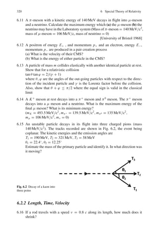
![4.2 Problems 251
where W is the number of accessible states.
Probability for finding a particle in the nth state at temperature T
P(n, T ) =
e−En/kT
Σ∞
n=0e−En /kT
(4.35)
Stirling’s approximation
n! =
√
2πn nn
e−n
(4.36)
4.2 Problems
4.2.1 Kinetic Theory of Gases
4.1 Derive the formula for the velocity distribution of gas molecules of mass m at
Kelvin temperature T .
4.2 Assuming that low energy neutrons are in thermal equilibrium with the sur-
roundings without absorption and that the Maxwellian distribution for veloci-
ties is valid, deduce their energy distribution.
4.3 In Problem 4.1 show that the average speed of gas molecule ν =
√
8kT/πm.
4.4 Show that for Maxwellian distribution of velocities of gas molecules, the root
mean square of speed ν2
1/2
= (3kT/m)1/2
4.5 (a) Show that in Problem 4.1 the most probable speed of the gas molecules
νp = (2kT/m)1/2
(b) Show that the ratio νp : ν : ν2
1/2
::
√
2 :
√
8/π :
√
3
4.6 Estimate the rms velocity of hydrogen molecules at NT P and at 127◦
C
[Sri Venkateswara University 2001]
4.7 Find the rms speed for molecules of a gas with density of 0.3 g/l of a pressure
of 300 mm of mercury.
[Nagarjuna University 2004]
4.8 The Maxwell’s distribution for velocities of molecules is given by N(ν)dν =
2π N(m/2πkT )3/2
ν2
exp(−mν2
/2kT )dν
Calculate the value of 1/ν
4.9 The Maxwell’s distribution of velocities is given in Problem 4.8. Show that the
probability distribution of molecular velocities in terms of the most probable
velocity between α and α + dα is given by](https://image.slidesharecdn.com/1000-solved-problems-in-modern-physics-220626164600-18e7ea67/85/1000-solved-problems-in-modern-physics-pdf-343-320.jpg)
![252 4 Thermodynamics and Statistical Physics
N(α)dα =
4N
√
π
α2
e−α2
dα
where, α = ν/νp and νp = (2kT/m)1/2
.
4.10 Calculate the fraction of the oxygen molecule with velocities between 199 m/s
and 201 m/s at 27◦
C
4.11 Assuming that the hydrogen molecules have a root-mean-square speed of
1,270 m/s at 300 K, calculate the rms at 600 K.
4.12 Clausius had assumed that all molecules move with velocity v with respect
to the container. Under this assumption show that the mean relative velocity
νrel of one molecule with another is given by νrel = 4ν/3.
4.13 Estimate the temperature at which the root-mean-square of nitrogen molecule
in earth’s atmosphere equals the escape velocity from earth’s gravitational
field. Take the mass of nitrogen molecule = 23.24 amu, and radius of
earth = 6,400 km.
4.14 Calculate the fraction of gas molecules which have the mean-free-path in the
range λ to 2λ.
4.15 If ρ is the density, ν the mean speed and λ the mean free path of the
gas molecules, then show that the coefficient of viscosity is given by η = 1
3
ρ
ν λ.
4.16 At STP, the rms velocity of the molecules of a gas is 105
cm/s. The molecular
density is 3 × 1025
m−3
and the diameter (σ) of the molecule 2.5 × 10⁻¹⁰
m.
Find the mean-free-path and the collision frequency.
[Nagarjuna University 2000]
4.17 When a gas expands adiabatically its volume is doubled while its Kelvin tem-
perature is decreased by a factor of 1.32. Calculate the number of degrees of
freedom for the gas molecules.
4.18 What is the temperature at which an ideal gas whose molecules have an aver-
age kinetic energy of 1 eV?
4.19 (a) If γ is the ratio of the specific heats and n is the degrees of freedom then
show that for a perfect gas
γ = 1 + 2/n
(b) Calculate γ for monatomic and diatomic molecules without vibration.
4.20 If K is the thermal conductivity, η the coefficient of viscosity, Cν the specific
heat at constant volume and γ the ratio of specific heats then show that for the
general case of any molecule
K
ηCν
=
1
4
(9γ − 5)](https://image.slidesharecdn.com/1000-solved-problems-in-modern-physics-220626164600-18e7ea67/85/1000-solved-problems-in-modern-physics-pdf-344-320.jpg)
![254 4 Thermodynamics and Statistical Physics
4.30 Obtain the following T ds equation
T ds = CV dT + T αET dV
where ET = −V
∂ P
∂V
T
is the isothermal elasticity and α = 1
V
∂V
∂T
P
is the volume coefficient of expansion, S is the entropy and T the Kelvin
temperature.
4.31 Obtain the equation
T ds = CpdT − T V αdp
4.32 Obtain the equation
T ds = CV
∂T
∂ P
V
dP + CP
∂T
∂V
P
dV
4.33 Obtain the formula for the Joule–Thompson effect
ΔT =
[T (∂V/∂T )P − V ]ΔP
CP
4.34 (a) Show that for a perfect gas governed by the equation of state PV = RT
the Joule-Thompson effect does not take place.
(b) Show that for an imperfect gas governed by the equation of state
P +
a
V 2
(V − b) = RT , the Joule-Thompson effect is given by
ΔT =
1
CP
2a
RT
− b
ΔP.
4.35 Explain graphically the condition for realizing cooling in the Joule-Thompson
effect using the concept of the inversion temperature.
4.36 Prove that for any substance the ratio of the adiabatic and isothermal elastici-
ties is equal to the ratio of the two specific heats.
4.37 Prove that the ratio of the adiabatic to the isobaric pressure coefficient of
expansion is 1/(1 − γ ).
4.38 Show that the ratio of the adiabatic to the isochoric pressure coefficient is
γ/(γ − 1).
4.39 If U is the internal energy then show that for an ideal gas (∂U/∂V )T = 0.
[Nagarjuna University 2004]
4.40 Find the change in boiling point when the pressure on water at 100◦
C is
increased by 2 atmospheres. (L = 540 Calg−1
, volume of 1 g of steam =
1,677 cc)
[Nagarjuna University 2000]
4.41 If 1 g of water freezes into ice, the change in its specific volume is 0.091 cc
Calculate the pressure required to be applied to freeze 10 g of water at −1◦
C.
[Sri Venkateswara University 1999]](https://image.slidesharecdn.com/1000-solved-problems-in-modern-physics-220626164600-18e7ea67/85/1000-solved-problems-in-modern-physics-pdf-346-320.jpg)
![4.2 Problems 255
4.42 Calculate the change of melting point of naphthalene per atmospheric change
of pressure, given melting point = 80◦
C, latent heat = 35.5 cal/g, density of
solid = 1.145 g/cc and density of liquid = 0.981 g/cc
[University of Calcutta]
4.43 The total energy of blackbody radiation in a cavity of volume V at temperature
T is given by u = aV T 4
, where a = 4σ/c is a constant.
(a) Obtain an expression for the entropy S in terms of T, V and a.
(b) Using the expression for the free energy F, show that the pressure P = 1
3
u.
4.44 Given that the specific heat of Copper is 387 J/kg K−1
, calculate the atomic
mass of Copper in amu using Dulong Petit law.
4.2.3 Statistical Distributions
4.45 Calculate the ratio of the number of molecules in the lowest two rotational
states in a gas of H2 at 50 K (take inter atomic distance = 1.05 A◦
)
[University of Cambridge, Tripos 2004]
4.46 Consider a photon gas in equilibrium contained in a cubical box of volume
V = a3
. Calculate the number of allowed normal modes of frequency ω in the
interval dω.
4.47 Show that for very large numbers, the Stirling’s approximation gives
n! ∼
=
√
2πn nn
e−n
4.48 Show that the rotational level with the highest population is given by
J max(pop) =
√
I0kT
−
1
2
4.49 Assuming that the moment of inertia of the H2 molecule is 4.64×10−48
kg-m2
,
find the relative population of the J = 0, 1, 2 and 3 rotational states at 400 K.
4.50 In Problem 4.49, at what temperature would the population for the rotational
states J = 2 and J = 3 be equal.
4.51 Calculate the relative numbers of hydrogen atoms in the chromosphere with
the principal quantum numbers n = 1, 2, 3 and 4 at temperature 6,000 K.
4.52 Calculate the probability that an allowed state is occupied if it lies above the
Fermi level by kT , by 5kT , by 10 kT .
4.53 If n is the number of conduction electrons per unit volume and m the electron
mass then show that the Fermi energy is given by the expression
EF =
h2
8m
3n
π
2/3](https://image.slidesharecdn.com/1000-solved-problems-in-modern-physics-220626164600-18e7ea67/85/1000-solved-problems-in-modern-physics-pdf-347-320.jpg)
![256 4 Thermodynamics and Statistical Physics
4.54 The probability for occupying the Fermi level PF = 1/2. If the probability for
occupying a level ΔE above EF is P+ and that for a level ΔE below EF is P−,
then show that for ΔE
kT
1, PF is the mean of P+ and P−
4.55 Find the number of ways in which two particles can be distributed in six states
if
(a) the particles are distinguishable
(b) the particles are indistinguishable and obey Bose-Einstein statistics
(c) the particles are indistinguishable and only one particle can occupy any
one state.
4.56 From observations on the intensities of lines in the optical spectrum of nitro-
gen in a flame the population of various vibrationally excited molecules rela-
tive to the ground state is found as follows:
v 0 1 2 3
Nv/N0 1.000 0.210 0.043 0.009
Show that the gas is in thermodynamic equilibrium in the flame and calcu-
late the temperature of the gas (θv = 3,350 K)
4.57 How much heat (in eV) must be added to a system at 27◦
C for the number of
accessible states to increase by a factor of 108
?
4.58 The counting rate of Alpha particles from a certain radioactive source shows
a normal distribution with a mean value of 104
per second and a standard
deviation of 100 per second. What percentage of counts will have values
(a) between 9,900 and 10,100
(b) between 9,800 and 10,200
(c) between 9,700 and 10,300
4.59 A system has non-degenerate energy levels with energy E =
n + 1
2
ω,
where ω = 8.625×10⁻⁵
eV, and n = 0, 1, 2, 3 . . . Calculate the probability
that the system is in the n = 10 state if it is in contact with a heat bath at room
temperature (T = 300 K). What will be the probability for the limiting cases
of very low temperature and very high temperature?
4.60 Derive Boltzmann’s formula for the probability of atoms in thermal equilib-
rium occupying a state E at absolute temperature T .
4.2.4 Blackbody Radiation
4.61 A wire of length 1 m and radius 1 mm is heated via an electric current to pro-
duce 1 kW of radiant power. Treating the wire as a perfect blackbody and
ignoring any end effects, calculate the temperature of the wire.
[University of London]](https://image.slidesharecdn.com/1000-solved-problems-in-modern-physics-220626164600-18e7ea67/85/1000-solved-problems-in-modern-physics-pdf-348-320.jpg)
![4.2 Problems 257
4.62 When the sun is directly overhead, the thermal energy incident on the earth is
1.4 kWm−2
. Assuming that the sun behaves like a perfect blackbody of radius
7 × 10⁵
km, which is 1.5 × 10⁸
km from the earth show that the total intensity
of radiation emitted from the sun is 6.4 × 10⁷
Wm−2
and hence estimate the
sun’s temperature.
[University of London]
4.63 If u is the energy density of radiation then show that the radiation pressure is
given by Prad = u/3.
4.64 If the temperature difference between the source and surroundings is small
then show that the Stefan’s law reduces to Newton’s law of cooling.
4.65 The pressure inside the sun is estimated to be of the order of 400 million atmo-
spheres. Estimate the temperature corresponding to such a pressure assuming
it to result from the radiation.
4.66 The mass of the sun is 2 × 1030
Kg, its radius 7 × 10⁸
m and its effective
surface temperature 5,700 K.
(a) Calculate the mass of the sun lost per second by radiation.
(b) Calculate the time necessary for the mass of the sun to diminish by 1%.
4.67 Compare the rate of fall of temperature of two solid spheres of the same
material and similar surfaces, where the radius of one surface is four times
of the other and when the Kelvin temperature of the large sphere is twice that
of the small one (Assume that the temperature of the spheres is so high that
absorption from the surroundings may be ignored).
[University of London]
4.68 A cavity radiator has its maximum spectral radiance at a wavelength of 1.0 μm
in the infrared region of the spectrum. The temperature of the body is now
increased so that the radiant intensity of the body is doubled.
(a) What is the new temperature?
(b) At what wavelength will the spectral radiance have its maximum value?
(Wien’s constant b = 2.897 × 10⁻³
m-K)
4.69 In the quantum theory of blackbody radiation Planck assumed that the oscil-
lators are allowed to have energy, 0, ε, 2ε . . . Show that the mean energy of
the oscillator is ε̄ = ε/[exp(ε/kT ) − 1] where ε = hν
4.70 Planck’s formula for the blackbody radiation is
uλdλ =
8πhc
λ5
1
ehc/λkT − 1
dλ
(a) Show that for long wavelengths and high temperatures it reduces to
Rayleigh-Jeans law.
(b) Show that for short wavelengths it reduces to Wien’s distribution law
4.71 Starting from Planck’s formula for blackbody radiation deduce Wien’s dis-
placement law and calculate Wien’s constant b, assuming the values of h, c
and k.](https://image.slidesharecdn.com/1000-solved-problems-in-modern-physics-220626164600-18e7ea67/85/1000-solved-problems-in-modern-physics-pdf-349-320.jpg)
![258 4 Thermodynamics and Statistical Physics
4.72 Using Planck’s formula for blackbody radiation show that Stefan’s constant
σ =
2
15
π5
k4
h3c2
= 5.67 × 10⁻⁸
W.m−2
.K−4
4.73 A blackbody has its cavity of cubical shape. Determine the number of modes
of vibration per unit volume in the wavelength region 4,990–5,010 A◦
.
[Osmania University 2004]
4.74 A cavity kept at 4,000 K has a circular aperture 5.0 mm diameter. Calculate (a)
the power radiated in the visible region (0.4–0.7 μm) from the aperture (b) the
number of photons emitted per second in the visible region
4.75 Planck’s formula for the black body radiation is
uλdλ =
8πhc
λ5
1
ehc/λkT − 1
dλ
Express this formula in terms of frequency.
4.76 Estimate the temperature TE of the earth, assuming that it is in radiation
equilibrium with the sun (assume the radius of sun Rs = 7 × 10⁸
m, the
earth-sun distance r = 1.5 × 10¹¹
m, the temperature of solar surface Ts =
5,800 K)
4.77 Calculate the solar constant, that is the radiation power received by 1 m2
of earth’s surface. (Assume the sun’s radius Rs = 7 × 10⁸
m, the earth-
sun distance r = 1.5 × 10¹¹
m, the earth’s radius RE = 6.4 × 10⁶
m,
sun’s surface temperature, Ts = 5,800 K and Stefan-Boltzmann constant
σ = 5.7 × 10⁻⁸ W
m2 − K4
).
4.78 A nuclear bomb at the instant of explosion may be approximated to a black-
body of radius 0.3 m with a surface temperature of 107
K. Show that the bomb
emits a power of 6.4 × 10²⁰
W.
4.3 Solutions
4.3.1 Kinetic Theory of Gases
4.1 Consider a two-body collision between two similar gas molecules of initial
velocity ν1 and ν2. After the collision, let the final velocities be ν3 and ν4.
The probability for the occurrence of such a collision will be proportional to
the number of molecules per unit volume having these velocities, that is to
the product f (ν1) f (ν2). Thus the number of each collisions per unit volume
per unit time is c f (ν1) f (ν2) where c is a constant. Similarly, the number of
inverse collisions per unit volume per unit time is c
f (ν3) f (ν4) where c
is
also a constant. Since the gas is in equilibrium and the velocity distribution is
unchanged by collisions, these two rates must be equal. Further in the centre](https://image.slidesharecdn.com/1000-solved-problems-in-modern-physics-220626164600-18e7ea67/85/1000-solved-problems-in-modern-physics-pdf-350-320.jpg)
![4.3 Solutions 261
4.5 (a) νp is found by maximizing the Maxwellian distribution.
d
dν
[ν2
exp(−mν2
/2kT )] = 0
exp(−mν2
/kT )[2ν − mν3
/kT ] = 0
whence ν = νp = (2kT/m)1/2
(b) νp : ν : ν2
1/2
:: (2kT/m)1/2
: (8kT/πm)1/2
: (3kT/m)1/2
=
√
2 :
8/π :
√
3
4.6 ν2
1/2
=
3kT
m
1/2
=
3 × 1.38 × 10−23
× 273
1.67 × 10⁻²⁷
1/2
= 2,601 m/s at N.T.P
ν2
1/2
=
3 × 1.38 × 10−23
× 400
1.67 × 10⁻²⁷
1/2
= 3,149 m/s at 127◦
C.
4.7 ν2
1/2
=
3p
ρ
1/2
=
3 × (300/760) × 1.013 × 105
0.3
1/2
= 632 m/s
4.8
1
ν
=
1
N
∞
0
1
ν
N(ν) dν
=
1
N
∞
0
1
ν
.4π N
m
2πkT
3/2
v2
exp(−mν2
/2kT ) dν
Set mν2
/2kT = x; vdν = kT dx/m
1
ν
= (2m/πkT )1/2
∞
0
exp(−x) dx = (2m/πkT )1/2
4.9 N(ν)dν = 4π N(m/2πkT )3/2
ν2
exp(−mv2
/2kT )dν (1)
νp = (2kT/m)1/2
(2)
Let ν/νp = α; dν = νpdα (3)
Use (2) and (3) in (1)
N(α)dα =
4N
√
π
α2
exp(−α2
)dα
4.10 Fraction
f =
N(ν)dv
N
= 4π
* m
2πkT
+3/2
ν2
exp(−mν2
/2kT )dν
ν =
199 + 201
2
= 200 m/s
dν = 201 − 199 = 2 m/s](https://image.slidesharecdn.com/1000-solved-problems-in-modern-physics-220626164600-18e7ea67/85/1000-solved-problems-in-modern-physics-pdf-354-320.jpg)
1/2
= 1270 ×
√
2 = 1,796 m/s
4.12 Relative velocity νrel of one molecule and another making an angle θ is
νrel = (ν2
+ ν2
− 2(ν)(ν) cos θ)1/2
= 2ν sin(θ/2)
Now, all the direction of velocities v are equally probable. The probability
f (θ) that v lies within an element of solid angle between θ and θ +dθ is given
by
f (θ) = 2πsin θdθ/4π =
1
2
sin θdθ
νrel is obtained by integrating over f (θ) in the angular interval 0 to π.
νrel =
π
0
νrel f (θ) =
π
0
2ν sin
θ
2
1
2
sin θdθ
= 2ν
π
0
sin2
θ
2
cos
θ
2
dθ = 4ν
π
0
sin2 θ
2
d
sin
θ
2
= 4ν/3
4.13 νe = (2gR)1/2
; νrms = (3kT/m)1/2
νrms = νe
T =
2mgR
3k
=
2 × (2 × 23.24 × 10−27
)(9.8)(6.37 × 10⁶
)
3 × 1.38 × 10−23
= 1.4 × 10⁵
K
4.14 Fraction of gas molecules that do not undergo collisions after path length x
is exp(−x/λ). Therefore the fraction of molecules that has free path values
between λ to 2λ is
f = exp(−λ/λ) − exp(−2λ/λ)
= exp(−1) − exp(−2)
= 0.37 − 0.14 = 0.23
4.15 Consider a volume element dV = 2πr2
sin θdθdr located on a layer at a
height z = r cos θ. If mu is the momentum of a molecule at the XY-plane
at z = 0, then its value at dV will be mu +
d
dz
mu
r cos θ (Fig. 4.2). At an
identical layer below the reference plane dA, the momentum would be](https://image.slidesharecdn.com/1000-solved-problems-in-modern-physics-220626164600-18e7ea67/85/1000-solved-problems-in-modern-physics-pdf-355-320.jpg)
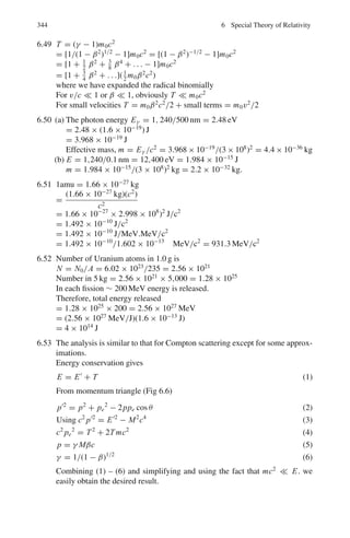
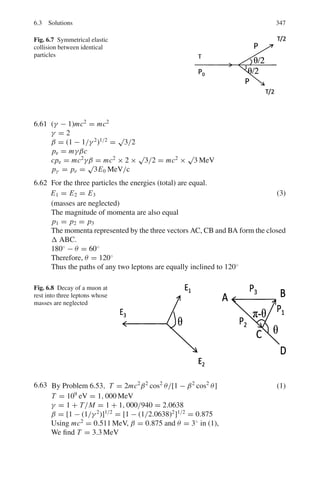
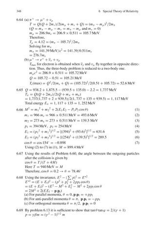
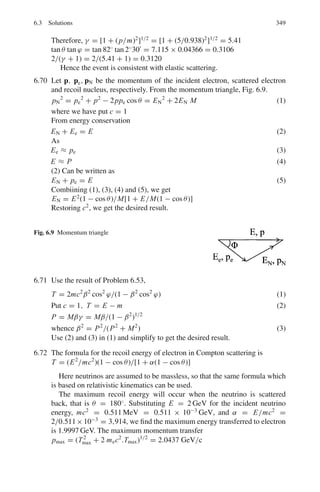
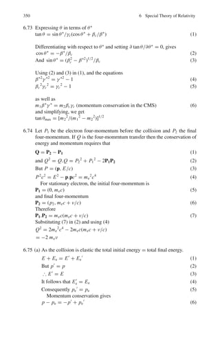
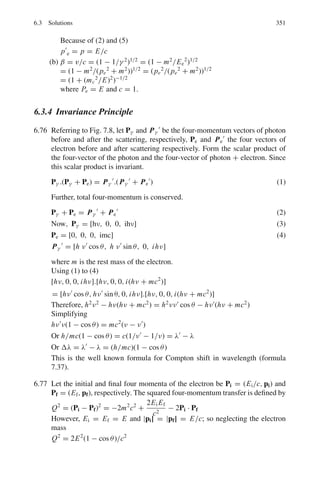
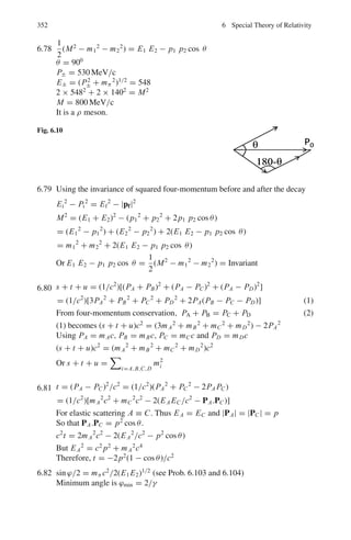
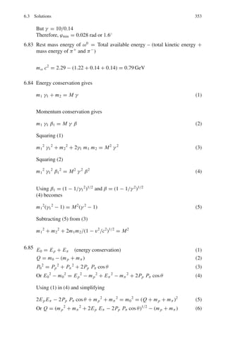
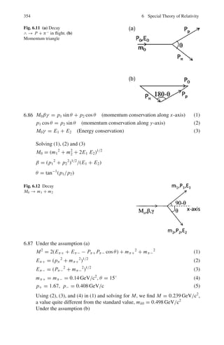
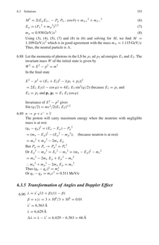
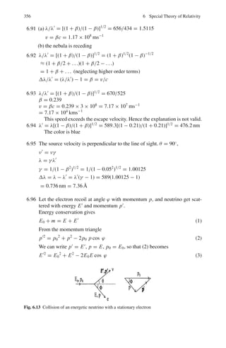
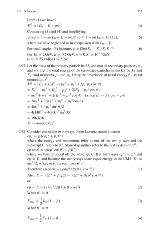
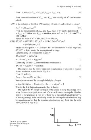
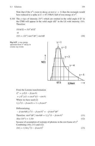
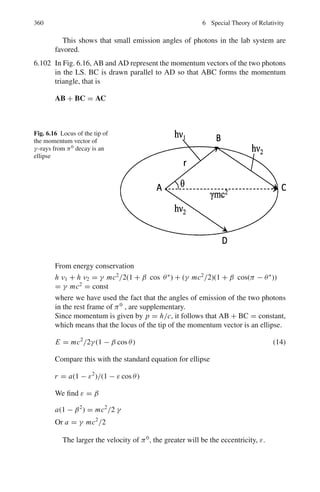
![4.3 Solutions 287
4.67 Power radiated, P = σ AT 4
= 4π R2
σ T 4
P2
P1
=
R2
2
R2
1
.
T 4
2
T4
1
=
(4R1)2
R2
1
.
(2T1)4
T4
1
= 256
Furthermore,
P2
P1
=
dQ2/dt
dQ1/dt
=
m2s(dT/dt)2
m1s(dT/dt)1
where s is the specific heat
But m2 ∝ R3
2 and m1 ∝ R3
1
∴
(dT/dt)2
(dT/dt)1
=
P2
P1
.
R3
1
R3
2
=
256
43
= 4
4.68 (a) λm.T = b
T =
b
λm
=
2.897 × 10⁻³
1 × 10−6
= 2,897 K
P2
P1
=
T 4
2
T 4
1
= 2
New temperature, T2 = T1 × 21/4
= 2,897 × 1.189 = 3,445K
(b) The wavelength at which the radiation has maximum intensity
λm =
2.897 × 10⁻³
3445
= 0.84 × 10⁻⁶
m = 0.84 μm
4.69 The mean value ∈ is determined from;
∈ =
Σ∞
n=0n ∈ e−βn∈
Σ∞
n=0e−βn∈
= −
d
dβ
ln
∞
n=0
e−βn∈
= −
d
dβ
ln
1 + e−β∈
+ e−2β∈
+ · · ·
= −
d
dβ
ln
1
1 − e−β∈
where we have used the formula for the sum of terms of an infinite geometric
series.
∈ =
∈ e−β∈
1 − e−β∈
=
∈
eβ∈ − 1
(β = 1/kT )
4.70 (a)
uλdλ =
8πhc
λ5
.
1
ehc/λkT − 1
dλ (Planck’s formula) (1)
For long wavelengths (low frequencies) and high temperatures the ratio
hc
λkT
1 so that we can expand the exponential in (1) and retain only the
first two terms
uλdλ =
8πhc
λ5[(1 + hc/λkT + . . .) − 1]
=
8πkT
λ4
dλ
writing λ = c
υ
; dλ = − c
υ2 dν](https://image.slidesharecdn.com/1000-solved-problems-in-modern-physics-220626164600-18e7ea67/85/1000-solved-problems-in-modern-physics-pdf-380-320.jpg)

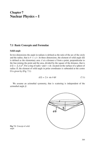
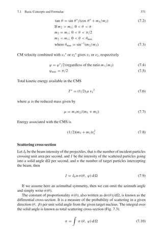
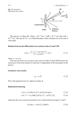
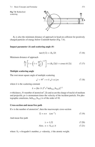
![298 5 Solid State Physics
nenh = 2.33 × 1031
T 3
e−Eg/kT
where Eg is the gap width
5.38 The effective mass m∗
of an electron or hole in a band is defined by
1
m∗
=
1
2
·
d2
E
dk2
where k is the wave number (k = 2π/λ). For a free electron show that
m∗
= m.
5.39 After adding an impurity atom that donates an extra electron to the conduction
band of silicon (μn = 0.13 m2
/Vs), the conductivity of the doped silicon is
measured as 1.08 (Ωm−1
). Determine the doped ratio (density of silicon is
2,420 kg/m3
).
5.40 Estimate the ratio of the electron densities in the conduction bands of silicon
(Eg = 1.14 eV) and germanium (Eg = 0.7 eV) at 400 K.
5.41 Show that at the room temperature (300 K) the electron densities in the con-
duction bands of the insulator carbon (Eg = 5.33 eV) and the semiconductor
like germanium (Eg = 0.7 eV) is extremely small.
5.42 A current of 8×10⁻¹¹
A flows through a silicon p −n junction at temperature
27 ◦
C. Calculate the current for a forward bias of 0.5 V.
5.43 Calculate the depletion layer width for a pn junction with zero bias in ger-
manium, given that the impurity concentrations are Na = 1 × 10²³
m−3
and
Nd = 2 × 10²²
m−3
, respectively at T = 300 K, ∈r = 16 and contact potential
difference V0 = 0.8 V.
5.44 Consider the Shockley equation for the diode
I = I0 exp[(eV /kT) − 1]
Show that the slope resistance re of the I − V curve at a particular d.c bias
is given to a good approximation, at room temperature (T = 300 K) by the
expression re = 26
I
Ω (forward bias) where I is in milliampere, and that for
the reverse bias re tends to infinity.
5.45 Given that a piece of n-type silicon contains 8 × 10²¹
m−3
phosphorus impu-
rity atoms, calculate the carrier concentrations at room temperature. It may be
assumed that the intrinsic electron concentration in silicon at room tempera-
ture is 1.6 × 10¹⁶
m−3
.
5.2.5 Superconductor
5.46 It is required to break up a Cooper pair in lead which has the energy gap of
2.73 eV. What is the maximum wavelength of photon which will accomplish
the job?](https://image.slidesharecdn.com/1000-solved-problems-in-modern-physics-220626164600-18e7ea67/85/1000-solved-problems-in-modern-physics-pdf-391-320.jpg)
![300 5 Solid State Physics
5.2 Volume of the unit cell = a3
. Since there are two atoms per unit cell, 8 × 1/8
for the corner atoms and 1 × 1 for the centre atom,
Volume = 2 ×
4
3
πr3
Since the body diagonal atoms touch one another,
4r = a
√
3
Volume of atoms in terms of a is
2 ×
4
3
πr3
= 2 ×
4
3
π[a
√
3/4]3
=
√
3πa3
/8
Or the fraction of the volume occupied by the body-centred cubic structure is
√
3π/8.
5.3
2d sin θ = nλ
d1 =
1.λ
2 sin θ
=
0.1
2 sin 4◦
= 0.717 nm
d2 =
0.1
2 sin 8◦
= 0.359 nm
5.4 nλ =
2a
(h2 + k2 + l2)1/2
sin θ =
2 × 0.4
(12 + 12 + 12)1/2
sin θ
sin θ =
0.3
√
3
0.8
= 0.6495
θ = 40.5◦
5.5 2d sin θ = nλ
d =
1.λ
2 sin θ
=
0.16
2 sin 30◦
= 0.136 nm
For n = 2,
sin θ =
2 × 0.16
2 × 0.136
= 1.176
a value which is not possible. Thus higher order reflections are not possible.
5.6 The de Broglie wavelength for electrons is calculated from
λ =](https://image.slidesharecdn.com/1000-solved-problems-in-modern-physics-220626164600-18e7ea67/85/1000-solved-problems-in-modern-physics-pdf-393-320.jpg)
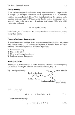
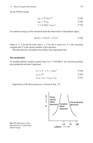


![310 5 Solid State Physics
5.39 The number of silicon atoms/m3
n =
N0d
A
=
6.02 × 1026
× 2,420
28
= 0.52 × 1029
Let x be the fraction of impurity atom (donor). The general expression for the
conductivity is
σ = nneμn + npeμp
where nn and np are the densities of the negative and positive charge carriers.
Because nn np,
σ ∼
= nneμn = xnpeμn
x =
σ
npeμn
=
1.08
0.52 × 1029 × 1.6 × 10−19 × 0.13
=
9.985
1010
or 1 part in 109
.
Note that in normal silicon the conductivity is of the order of 10−4
(Ω− m)−1
.
A small fraction of doping (10−9
) has dramatically increased the value by four
orders of magnitude.
5.40 ne = (4.83 × 10²¹
)T 3/2
e−Eg/2kT
e/m3
nGe
nSi
= e(ESi−EGe)/2kT
kT =
1.38 × 10−23
× 400
1.6 × 10−19
= 0.0345 eV
nGe
nSi
= e(1.14−0.7)/(2×0.0345)
= 588
5.41 kT =
1.38 × 10−23
× 300
1.6 × 10−19
= 0.0259 eV
nC
nGe
= e−(EGe−EC )/2K T
= e−(5.33−07)/0.052
= e−89
≈ 2.2 × 10−39
5.42 I = I0[exp(eV/kT ) − 1]
where I0 is the forward bias saturation current.
I = 8×10⁻¹¹
exp
0.5 × 1.6 × 10−19
1.38 × 10−23 × 300
− 1
= 19.7×10⁻³
A = 19.7 mA
5.43 W =
20r
e
(V0 − Vb)
1
Na
+
1
Nd
1/2
where r is the relative permittivity, Vb is the bias voltage applied to the junc-
tion (here Vb = 0), Na and Nd are carrier concentrations in n-type and p-type
respectively.
W =
2 × 8.85 × 10−12
× 16 × 0.8
1.6 × 10⁻¹⁹
1
1 × 10²³
+
1
2 × 10²²
1/2
= 0.29 μm](https://image.slidesharecdn.com/1000-solved-problems-in-modern-physics-220626164600-18e7ea67/85/1000-solved-problems-in-modern-physics-pdf-410-320.jpg)
![5.3 Solutions 311
5.44 I = I0[exp(eV/kT ) − 1] (1)
1
re
=
dI
dV
=
eI0
kT
exp(eV/kT ) (2)
But exp (eV/kT) 1. Therefore
1
re
=
eI
kT
or re =
kT
eI
=
1.38 × 10−23
× 300
1.6 × 10⁻¹⁹ I
=
25.875 × 10⁻³
I
If I is in milliamp.
re ≈
26
I
(forward bias) (3)
For the reversed bias we note from (2)
1
re
=
dI
dV
=
e
kT
I0 exp (eV/kT ) = 0
For V ≤ −4kT/e,re → ∞. (reverse bias) (4)
5.45 For a semiconductor in equilibrium the product of n(= Nd) and p(= Na) is
equal to n2
i , the square of the intrinsic concentration.
n × p = n2
i
p =
n2
i
n
=
(1.6 × 10¹⁶
)2
8 × 1021
= 3.2 × 10¹⁰
m−3
5.3.5 Superconductor
5.46 λ =
1241
E(eV)
nm =
1, 241
2.73 × 10−3
= 4.546 × 10⁵
nm
5.47 Eg =
1241
λ(nm)
=
1, 241
1.08 × 106
= 1.15 × 10⁻³
eV
5.48 f =
2eV
h
=
2(1.602 × 10⁻¹⁹
)(1.5 × 10⁻⁶
)
6.626 × 10−34
= 7.253×10⁸
Hz = 0.7253 GHz
5.49 Eg = 3.53kTc = (3.53)
(1.38 × 10⁻²³
)
1.6 × 10⁻¹⁹
(3.4) = 1.035 × 10⁻³
eV
5.50 Tc(B) = Tc
1 −
B
Bc
1/2
2.0 = 7.19
1 −
0.074
Bc
1/2
Solving for Bc, we get Bc = 0.079 T .](https://image.slidesharecdn.com/1000-solved-problems-in-modern-physics-220626164600-18e7ea67/85/1000-solved-problems-in-modern-physics-pdf-411-320.jpg)
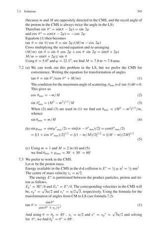
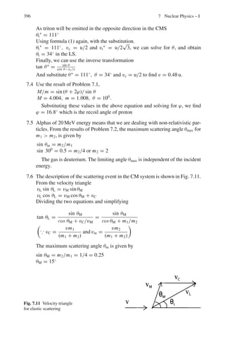
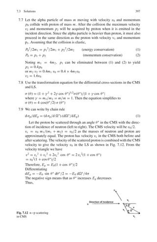
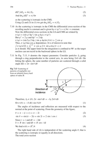
![318 6 Special Theory of Relativity
Inverse transformations
cpx = γ (cp
x + βE
) (6.41)
cpy = cp
y (6.42)
cpz = cp
z (6.43)
E = γ (E
− βcp
x∗ ) (6.44)
E 2
− c2
p 2
= E2
− c2
p2
= m2
0 = Invariant (6.45)
γ
= γ γ0(1 − ββ0 cos θ0) (6.46)
γ0 = γ γ
(1 + ββ∗
cos θ∗
) (6.47)
where zeros refer to the particle’s velocity, Lorentz factor and the angle in the
S-system while primes refer to the corresponding quantities in the S
system.
Transformation of angles
tan θ
=
sin θ
γ
cos θ − β
β0
(6.48)
tan θ =
sin θ
γc(cos θ − β/β )
(6.49)
Optical Doppler effect
ν
= γ ν(1 − β cos θ) (6.50)
ν = γ ν
(1 + β cos θ∗
) (6.51)
where ν is the frequency in the S-system and ν
is the frequency in the S
-system,
θ and θ
are the corresponding angles, β is the source velocity and γ is the corre-
sponding Lorentz factor.
Threshold for particle production
Consider the reaction
m1 + m2 → m3 + m4 + M (6.52)
T (threshold) =
1
2m2
[(m3 + m4 + M)2
− (m1 + m2)2
]
T (threshold) =
(Sum of final masses)2
− (sum of initial masses)2
2 × mass of target particle
(6.53)](https://image.slidesharecdn.com/1000-solved-problems-in-modern-physics-220626164600-18e7ea67/85/1000-solved-problems-in-modern-physics-pdf-418-320.jpg)
![6.2 Problems 319
6.2 Problems
6.2.1 Lorentz Transformations
6.1 In the inertial system S, an event is observed to take place at point A on the
x-axis and 10−6
S later another event takes place at point B, 900 m further
down. Find the magnitude and direction of the velocity of S
with respect to S
in which these two events appear simultaneous.
6.2 Show that the Lorentz-transformations connecting the S
and S systems may
be expressed as
x1
= x1 cosh α−ct sinh α
x2
= x2
x3
= x3
t
= t cosh α − (x1t sinh α)/c
where tanh α = ν/c. Also show that the Lorentz transformations correspond
to a rotation through an angle iα in four-dimensional space.
6.3 A pion moving along x-axis with β = 0.8 in the lab system decays by emitting
a muon with β
= 0.268 along the incident direction (x
-axis) in the rest
system of pion. Find the velocity of the muon (magnitude and direction) in the
lab system.
6.4 In Problem 6.3, the muon is emitted along the y
-axis. Find the velocity of
muon in the lab frame
6.5 In Problem 6.3, the muon is emitted along the positive y-axis (i.e. perpendic-
ular to the incidental direction of pion in the lab frame). Find the speed of
muon in the lab frame and the direction of emission in the rest frame of pion.
Assume βc = 0.2
6.6 Show that Maxwell’s equations for the propagation of electromagnetic waves
are Lorentz invariant.
6.7 A neutral K meson decays in flight via K0
→ π+
π−
. If the negative pion is
produced at rest, calculate the kinetic energy of the positive pion.
[Mass of K0
is 498 MeV/c2
; that of π±
is 140 MeV/c2
]
6.8 A pion travelling with speed ν = |ν| in the laboratory decays via π → μ + ν.
If the neutrino emerges at right angles to ν, find an expression for the angle θ
at which the muon emerges.
6.9 Determine the speed of the Lorentz transformation in the x-direction for which
the velocity in the frame S of a particle is u = (c/
√
2, c/
√
2) and the velocity
in frame S
is seen as
u
= (−c/
√
2, c/
√
2).
6.10 A particle decays into two particles of mass m1 and m2 with a release of energy
Q. Calculate relativistically the energy carried by the decay products in the
rest frame of the decaying particle.](https://image.slidesharecdn.com/1000-solved-problems-in-modern-physics-220626164600-18e7ea67/85/1000-solved-problems-in-modern-physics-pdf-419-320.jpg)
![320 6 Special Theory of Relativity
6.11 A π-meson with a kinetic energy of 140 MeV decays in flight into μ-meson
and a neutrino. Calculate the maximum energy which (a) the μ-meson (b) the
neutrino may have in the Laboratory system (Mass of π-meson = 140 MeV/c2
,
mass of μ-meson = 106 MeV/c, mass of neutrino = 0)
[University of Bristol 1968]
6.12 A positron of energy E+ , and momentum p+ and an electron, energy E−,
momentum p− are produced in a pair creation process
(a) What is the velocity of their CMS?
(b) What is the energy of either particle in the CMS?
6.13 A particle of mass m collides elastically with another identical particle at rest.
Show that for a relativistic collision
tan θ tan ϕ = 2/(γ + 1)
where θ, ϕ are the angles of the out-going particles with respect to the direc-
tion of the incident particle and γ is the Lorentz factor before the collision.
Also, show that θ + ϕ ≤ π/2 where the equal sign is valid in the classical
limit
6.14 A K+
meson at rest decays into a π+
meson and π0
meson. The π+
meson
decays into a μ meson and a neutrino. What is the maximum energy of the
final μ meson? What is its minimum energy?
(mK = 493.5 MeV/c2
, mπ+ = 139.5 MeV/c2
, mπ0 = 135 MeV/c2
,
mμ = 106 MeV/c2
, mν = 0)
6.15 An unstable particle decays in its flight into three charged pions (mass
140 MeV/c2
). The tracks recorded are shown in Fig. 6.2, the event being
coplanar. The kinetic energies and the emission angles are
T1 = 190 MeV, T2 = 321 MeV, T3 = 58 MeV
θ1 = 22.4◦
, θ2 = 12.25◦
Estimate the mass of the primary particle and identify it. In what direction was
it moving?
Fig. 6.2 Decay of a kaon into
three poins
6.2.2 Length, Time, Velocity
6.16 If a rod travels with a speed ν = 0.8 c along its length, how much does it
shrink?](https://image.slidesharecdn.com/1000-solved-problems-in-modern-physics-220626164600-18e7ea67/85/1000-solved-problems-in-modern-physics-pdf-420-320.jpg)
![322 6 Special Theory of Relativity
6.29 A spaceship is moving away from earth with speed ν = 0.6 c. When the ship
is at a distance d = 5 × 10⁸
km from earth. A radio signal is sent to the ship
by the observers on earth.
How long does the signal take to reach the ship as measured by the scientist
on earth?
6.30 In Problem 6.29, how long does the signal take to reach the ship as measured
by the crew of the spaceship?
6.31 If the mean track length of 100 MeV π mesons is 4.88 m up to the point of
decay, calculate their mean lifetime.
[University of Durham 1962]
6.32 A beam of π+
mesons of energy 1 GeV has an intensity of 106
particles per sec
at the beginning of a 10 m flight path. Calculate the intensity of the neutrino
flux at the end of the flight path (mass of π meson = 139 MeV/c2
, lifetime =
2.56 × 10⁻⁸
s)
[University of Durham 1961]
6.33 A π+
meson at rest decays into a μ+
meson and a neutrino in 2.5 × 10⁻⁸
s.
Assuming that the π+
meson has kinetic energy equal to its rest energy. What
distance would the meson travel before decaying as seen by an observer at rest?
6.34 Beams of high-energy muon neutrinos can be obtained by generating intense
beams of π+
mesons and allowing them to decay while in flight. What frac-
tion of the π+
mesons in a beam of momentum 200 GeV/c will decay while
travelling a distance of 300 m?
At the end of the decay path (an evacuated tunnel) the beam is a mixture of
π+
-mesons, muons and neutrinos. What distinguishes these particles in their
interactions with matter, and how is a neutrino beam free of contamination by
π-mesons and muons obtained? [π+
-meson mean-life: 2.6 × 10⁻⁸
s]
[Osmania University]
6.35 A beam of 140 MeV kinetic energy π+
mesons through three counters A, B,
C spaced 10 m apart. If 1,000 pions pass through counter A and 470 in B. (a)
how many pions are expected to be recorded in C? (b) Find the mean life time
of pions (Take mass of pion as 140 MeV/c2
)
6.36 A moving object heads toward a stationary one with a velocity αc. At what
velocity βc would an observer have to move so that in his frame of reference
the objects would have equal and opposite velocities?
6.37 A beam of identical unstable particles flying at a speed βc is sent through
two counters separated by a distance L. It is observed that N1 particles are
recorded at the first counter and N2 at the second counter, the reduction being
solely due to the decay of the particles in flight.
(i) Show that the lifetime of the particles at rest is given by
τ =
L
ln
N1
N2
(
γ 2 − 1 c](https://image.slidesharecdn.com/1000-solved-problems-in-modern-physics-220626164600-18e7ea67/85/1000-solved-problems-in-modern-physics-pdf-422-320.jpg)
![6.2 Problems 323
where the Lorentz factor γ is defined as usual
(ii) Hence determine the lifetime of muons at rest, knowing that when trav-
elling at a speed c
√
8/3 through the apparatus described above (with L =
200 m) N1 and N2 were measured to be 10,000 and 8,983, respectively.
[adapted from University of London, Royal Holloway and Bedford New
College]
6.38 A particle X at rest is a sphere of rest-mass m and radius r and has a proper
lifetime τ. If the particle is moving with speed
√
3
2
c with respect to the lab
frame (c is the speed of light):
(a) Determine the total energy of the particle in the lab frame
(b) The average distance the particle travels in the lab before decaying
(c) Sketch the shape and dimensions of the particle when viewed perpendicular
to its motion in the lab frame, include an arrow to indicate its direction of
motion on your sketch.
[adapted from the University of London Royal Holloway and Bedford New
College 2006]
6.39 The Lorentz velocity transformation is ν
= ν−u
1−uν/c2 , where ν
and ν are the
velocities of an object parallel to u as measured in two inertial frames with
relative velocity u. Show that a photon moving at c, the speed of light will
have the same speed in all frames of reference.
6.2.3 Mass, Momentum, Energy
6.40 The mean life-time of muons at rest is 2.2 × 10⁻⁶
s. The observed mean life-
time of muons as measured in the laboratory is 6.6 × 10⁻⁶
s. Find
(a) The effective mass of a muon at this speed when its rest mass is 207 me
(b) its kinetic energy (c) its momentum
6.41 Calculate the energy that can be obtained from complete annihilation of 1 g of
mass.
6.42 What is the speed of a proton whose kinetic energy equals its rest energy?
Does the result depend on the mass of proton?
6.43 What is the speed of a particle when accelerated to 1.0 GeV when the
particle is (a) proton (b) electron
6.44 (a) Calculate the energy needed to break up the 12
C nucleus into its con-
stituents. The rest masses in amu are:
12
C 12.000000; p 1.007825; n 1.008665; α 4.002603
(b) If 12
C nucleus is to break up into 3 alphas. Calculate the energy that is
released.](https://image.slidesharecdn.com/1000-solved-problems-in-modern-physics-220626164600-18e7ea67/85/1000-solved-problems-in-modern-physics-pdf-423-320.jpg)
![324 6 Special Theory of Relativity
(c) If the alphas are to further break into neutrons and protons, then show that
the overall energy needed is identical with the results in (a)
6.45 The kinetic energy and the momentum of a particle deduced from mea-
surements on its track in nuclear photographic emulsions are 250 MeV and
368 MeV/c, respectively. Determine the mass of the particle in terms of elec-
tron mass and identify it.
[University of Durham]
6.46 What is the rest mass energy of an electron (me = 9.1 × 10⁻³¹
kg)?
6.47 What potential difference is required to accelerate an electron from rest to
velocity 0.6 c?
6.48 At what velocity does the relativistic kinetic energy differ from the classical
energy by
(a) 1% (b) 10%?
6.49 Prove that if ν/c 1, the kinetic energy of a particle will be much less
than its rest energy. Further show that the relativistic expression reduces to the
classical one for small velocities.
6.50 Find the effective mass of a photon for
(a) λ = 5,000Å (visible region) (b) λ = 1Å (X-ray region)
6.51 Show that 1 amu = 931.5 MeV/c2
6.52 Estimate the energy that is released in the explosion of a fission bomb con-
taining 5.0 kg of fissionable material
6.53 A proton moving with a velocity βc collides with a stationary electron of mass
m and knocks it off at an angle θ with the incident direction. Show that the
energy imparted to the electron is approximately
T = 2mc2
β2
cos2
θ/(1 − β2
cos2
θ)
6.54 A positive pion (mπ = 273 me) decays into a muon (mμ = 207 me) and
a neutrino (mν = 0) at rest. Calculate the energy carried by the muon and
neutrino, given that mec2
= 0.511 MeV
6.55 A body of rest mass m travelling initially at a speed of β = 0.6 makes a com-
pletely inelastic collision with an identical body initially at rest. Find (a) the
speed of the resulting body (b) its rest mass in terms of m.
6.56 A neutral particle is observed to decay into a kaon and a pion. They are pro-
duced in the opposite direction, each of them with momentum 861 MeV/c.
Calculate the mass of the neutral particle and identify it. (Mass of kaon is
494 MeV/c2
, Mass of pion is 140 MeV/c2
).
6.57 A pion at rest decays via π → μ + ν. Find the speed of the muon in terms of
the masses involved.](https://image.slidesharecdn.com/1000-solved-problems-in-modern-physics-220626164600-18e7ea67/85/1000-solved-problems-in-modern-physics-pdf-424-320.jpg)
![6.2 Problems 325
6.58 A particle A decays at rest via A → B + C. Find the total energy of B in
terms of the masses of A, B and C.
6.59 Calculate the maximum energy of the positron emitted in kaon decay at rest
K+
→ e+
+ π0
+ γe.
6.60 Consider a symmetric elastic collision between a particle of mass m and
kinetic energy T and a particle of the same mass at rest. Relativistically, show
that the cosine of the angle between the two particles after the collision is
T/(T + 4 mc2
)
6.61 An electron has kinetic energy equal to its rest energy. Show that the energy
of a photon which has the same momentum as this electron is given by
Eγ =
√
3E0, where E0 = mec2
6.62 Consider the decay of muon at rest. If the energy released is divided equally
among the final leptons, then show that the angle between paths of any two
leptons is approximately 120◦
(neglect the mass of leptons compared to the
mass of muon mass).
6.63 If a proton of 109
eV collides with a stationary electron and knock it off at
3◦
with respect to the incident direction, what is the energy acquired by the
electron?
[Osmania University 1963]
6.64 Calculate (a) the mass of the pion in terms of the mass of the electron, given
that the kinetic energy of the muon from the pion decay at rest is 4.12 MeV
and (b) the maximum energy of electron (in MeV) from the decay of muon
at rest (mass of muon is 206.9 me). The mass of the electron is equivalent to
0.511 MeV)
[University of Durham 1961]
6.65 Antiprotons are captured at rest in deuterium giving rise to the reaction.
p−
+ d → n + π0
Find the total energy of the π0
. The rest energies for p−
, d, n, π0
are 938.2,
1875.5, 939.5 and 135.0 MeV respectively.
6.66 As a result of a nuclear interaction a K∗+
particle is created which decays to a
K meson and a π−
meson with rest masses equal to 966 me and 273 me respec-
tively. From the curvature of the resulting tracks in a magnetic field, it is con-
cluded that the momentum of the secondary K and π mesons are 394 MeV/c
and 254 MeV/c respectively, their initial directions of motion being inclined
to one another at 154◦
. Calculate the rest mass of the K∗
particle
[Bristol 1964, 1966]
6.67 A proton of kinetic energy 940 MeV makes an elastic collision with a station-
ary proton in such a way that after collision, the protons are travelling at equal
angles on either side of the incident proton. Calculate the angle between the
directions of motion of the protons.
[Liverpool 1963]](https://image.slidesharecdn.com/1000-solved-problems-in-modern-physics-220626164600-18e7ea67/85/1000-solved-problems-in-modern-physics-pdf-425-320.jpg)
![326 6 Special Theory of Relativity
6.68 A proton of momentum p large compared with its rest mass M, collides with
a proton inside a target nucleus with Fermi momentum pf. Find the available
kinetic energy in the collision, as compared with that for a free-nucleon target,
when p and pf are (a) parallel (b) anti parallel (c) orthogonal.
6.69 An antiproton of momentum 5 GeV/c suffers a scattering. The angles of the
recoil proton and scattered antiproton are found to be 82◦
and 2◦
30
with
respect to the incident direction. Show that the event is consistent with an
elastic scattering of an antiproton with a free proton.
6.70 Show that if E is the ultra-relativistic laboratory energy of electrons incident
on a nucleus of mass M, the nucleus will acquire kinetic energy
EN = (E2
/Mc2
)(1 − cos θ)/(1 + E(1 − cos θ)/Mc2
)
where θ is the scattering angle.
6.71 A particle of mass M me scatters elastically from an electron. If the inci-
dent particle’s momentum is p and the scattered electron’s relativistic energy
is E and φ is the angle the electron makes with the incident particle, show that
M = P[{[E + me]/[E − me]} cos2
φ − 1]]1/2
6.72 A neutrino of energy 2 GeV collides with an electron. Calculate the maximum
momentum transfer to the electron.
6.73 A particle of mass m1 collides elastically target particle of mass m2 at rela-
tivistic energy. Show that the maximum angle at which m1 is scattered in the
lab system is dependent only on the masses of particles provided m1 m2
6.74 Show that if energy ν( mec2
) and momentum q are transferred to a free sta-
tionary electron the four-momentum transfer squared is given by q2
= −2meν
6.75 A photon of energy E travelling in the +x direction collides elastically with
an electron of mass m moving in the opposite direction. After the collision,
the photon travels back along the –x direction with the same energy E.
(a) Use the conservation of energy and momentum to demonstrate that the
initial and final electron momenta are equal and opposite and of magni-
tude E/c.
(b) Hence show that the electron speed is given by
v/c = (1 + (mc
2
/E)2
)−1/2
[adapted from the University of Manchester 2008]
6.2.4 Invariance Principle
6.76 Use the invariance of scalar product of two four-vectors under Lorentz trans-
formation to obtain the expression for Compton scattering wavelength shift.
6.77 Show that for a high energy electron scattering at an angle θ, the value of
the squared four-momentum transfer is given approximately by Q2
= 2E2](https://image.slidesharecdn.com/1000-solved-problems-in-modern-physics-220626164600-18e7ea67/85/1000-solved-problems-in-modern-physics-pdf-426-320.jpg)
![6.2 Problems 327
(1 − cos θ)/c2
, where E is the total initial electron’s energy in the lab system.
State when this approximation is justified.
6.78 A neutral unstable particle decays into π+
and π−
, each of which has a
momentum 530 MeV/c. The angle between the two pions is 90◦
. Calculate
the mass of the unstable particle.
6.79 If a particle of mass M decays in flight into m1 and another m2; m1 has
momentum p1 and total energy E1, where as m2 has momentum p2 and total
energy E2. p1 and p2 make an angle θ. Show that
E1 E2 − p1 p2 cos θ = invariant = 1
2
[M2
− m1
2
− m2
2
]
6.80 The Mandelstam variables s, t, and u are defined for the reaction A + B →
C + D, by
s = (PA + PB)2
/c2
, t = (PA − PC)2
/c2
, u = (PA − PD)2
/c2
where PA, PB, PC, PD are the relevant energy-momentum four vectors. Show
that
s + t + u =
mj
2
( j = A, B, C, D)
6.81 In Problem 6.80 show for the elastic scattering t = −2p2
(1−cos θ)/c2
where
p = |p|.p is the center of mass momentum of particle and θ is its scattering
angle in the CMS.
6.82 A neutral pion undergoes radioactive decay into two γ -rays. Obtain the
expression for the laboratory angle between the direction of the γ -rays,
and find the minimum value for the angle when the pion energy is 10 GeV
(mπ = 0.14 GeV)
[University of Bristol 1965]
6.83 A bubble chamber event was identified in the reaction
p−
+ p → π+
+ π−
+ ω0
The total energy available was 2.29 GeV while the kinetic energy of the resid-
ual particles was 1.22 GeV. What is the rest energy of ω0
in MeV?
6.84 A particle of rest mass m1 and velocity v1 collides with a particle of mass
m2 at rest after which the two particles coalesce. Show that the mass M
and velocity v of the composite particle are related by M2
= m1
2
+ m2
2
+
2m1m2/
1 − v2/c2
6.85 Show that for the decay in flight of a Λ-hyperon into a proton and a pion with
Laboratory momenta Pp and Pπ respectively, the Q value can be calculated
from
Q = (mp
2
+ mπ
2
+ 2Ep Eπ − 2Pp Pπ cos θ)1/2
− (mp + mπ )
where θ is the angle between Pp and Pπ in the Laboratory system and E is
the total relativistic energy
[University of Dublin 1967]
6.86 Two particles are moving with relativistic velocities in directions at right
angles, they have momenta p1 and p2 and total energies E1 and E2. If they](https://image.slidesharecdn.com/1000-solved-problems-in-modern-physics-220626164600-18e7ea67/85/1000-solved-problems-in-modern-physics-pdf-427-320.jpg)
![328 6 Special Theory of Relativity
are the sole products of disintegration of a heavier object, what was the rest
mass, velocity and direction of motion?
[University of Bristol 1965]
6.87 A V-type of event is observed in a bubble chamber. The curvature measure-
ments on the two tracks show that their momenta are p+ = 1.670 GeV/c and
p− = 0.408 GeV/c. The angle contained between the two tracks is θ = 15◦
. It
is obviously due to the decay of a neutral unstable particle. It is suspected that
it is due to the decay (a) K0
→ π+
+ π−
or (b) Λ → p + π−
. Identify the
neutral particle.
6.88 Derive the formula in Problem 6.103 using the invariance of (ΣE)2
− |Σp|2
6.89 Calculate the maximum four momentum transfer to proton in the decay of
neutron at rest.
6.2.5 Transformation of Angles and Doppler Effect
6.90 Find the Doppler shift in wavelength of H line at 6,563 Å emitted by a star
receding with a relative velocity of 3 × 10⁶
ms−1
.
6.91 Certain radiation of a distant nebula appears to have a wavelength 656 nm
instead of 434 nm as observed in the laboratory. (a) if the nebula is mov-
ing in the line of sight of the observer, what is its speed? (b) Is the nebula
approaching or receding?
6.92 Show that for slow speeds, the Doppler shift can be approximated as
Δλ/λ = v/c
where Δλ is the change in wavelength.
6.93 A physicist was arrested for going over the railway level crossing on a motor-
cycle when the lights were red. When he was produced before the magistrate
the physicist declared that he was not guilty as red lights (λ = 670 nm)
appeared green (λ = 525 nm) due to Doppler Effect. At what speed he was
travelling for the explanation to be valid? Do you think such a speed is
feasible?
6.94 A spaceship is receding from earth at a speed of 0.21 c. A light from the
spaceship appears as yellow (λ = 589.3 nm) to an observer on earth. What
would be its color as seen by the passenger of the spaceship?
6.95 Find the wavelength shift in the Doppler effect for the sodium line 589 nm
emitted by a source moving in a circle with a constant speed 0.05 c observed
by a person fixed at the center of the circle.
6.96 A neutrino of energy E0 and negligible mass collides with a stationary elec-
tron. Find an expression for the laboratory angle of emission of the electron
in terms of its recoil energy E and calculate its value when E0 = 2 GeV and
E = 0.5 GeV](https://image.slidesharecdn.com/1000-solved-problems-in-modern-physics-220626164600-18e7ea67/85/1000-solved-problems-in-modern-physics-pdf-428-320.jpg)
![6.2 Problems 329
6.97 Assume the decay K0
→ π+
+π−
. Calculate the mass of the primary particle
if the momentum of each of the secondary particles is 3 × 10⁸
eV and the
angle between the tracks is 70◦
[University of Durham 1960]
6.98 Neutral pions of fixed energy decay in flight into two γ -rays. Show that the
velocity of pion is given by
β = (Emax − Emin)/(Emax + Emin)
where E is the γ -ray energy in the laboratory
6.99 In Problem 6.98 show that the rest mass energy of π0
is given by mc2
=
2(Emax Emin)1/2
6.100 In Problem 6.98 show that the energy distribution of γ -rays in the laboratory
is uniform under the assumption that γ -rays are emitted isotropically in the
rest system of π0
6.101 In Problem 6.98 show that the angular distribution of γ -rays in the laboratory
is given by
I(θ) = 1/4πγ 2
(1 − β cos θ)2
6.102 In Problem 6.98 show that the locus of the tip of the momentum vector is an
ellipse
6.103 In Problem 6.98 show that in a given decay the angle φ between two γ -rays
is given by
sin(φ/2) = mc2
/2(E1 E2)1/2
6.104 In Problem 6.98 show that the minimum angle between the two γ -rays is
given by
φmin = 2mc2
/Eπ
6.105 In Problem 6.98 find an expression for the disparity D (the ratio of energies)
of the γ -rays and show that D 3 in half the decays and D 7 in one
quarter of them
6.106 In the interaction π−
+ p → K∗
(890) + Y0
∗
(1, 800) at pion momentum
10 GeV/c , K∗
is produced at an angle θ in the lab system. Calculate the
maximum value θm, given mπ = 0.140 GeV/c2
and mp = 0.940 GeV/c2
6.107 A particle of mass m1 travelling with a velocity v = βc collides elastically
with the particle m2 at rest. The scattering angles of m1 in the LS and CMS
are θ and θ∗
. Show that
(a) γc = (γ + ν)/(1 + 2γ ν + ν2
)1/2
(b) γ ∗
= (γ + 1/γ )/
√
(1 + 2γ/ν + 1/ν2
)
(c) tan θ = sin θ∗
/γc(cos θ∗
+ βc/β∗
)
(d) tan θ∗
= sin θ/γc(cos θ − βc/β∗
)
where βc is the CMS velocity, β∗
c is the velocity of m1 in CMS,
γc = (1 − βc
2
)−1/2
, γ ∗
= (1 − β∗2
)−1/2
, ν = m2/m1](https://image.slidesharecdn.com/1000-solved-problems-in-modern-physics-220626164600-18e7ea67/85/1000-solved-problems-in-modern-physics-pdf-429-320.jpg)
![330 6 Special Theory of Relativity
6.108 A linear accelerator produces a beam of excited carbon atoms of kinetic
energy 120 MeV. Light emitted on de-excitation is viewed at right angles
to the beam and has a wavelength λ
. If λ is the wavelength emitted by a
stationary atom, what is the value of (λ
− λ)/λ? (Take the rest energies of
both protons and neutrons to be 109
eV)
[University of Manchester 1970]
6.109 A certain spectral line of a star has natural frequency of 5 × 10¹⁷
c/s. If the
star is approaching the earth at 300 km/s, what would be the fractional change
of frequency?
6.110 A neutral pion (mass 135 MeV/c2
) travelling with speed β = v/c = 0.8
decays into two photons at right angle to the line of flight. Find the angle
between the two photons as observed in the lab system.
6.111 An observer O sights light coming to him by an object X at 45◦
to its path as
in the diagram. If the corresponding angle of emission of light in the frame
of reference of the object is 60◦
, calculate the velocity of the object.
Fig. 6.3 Aberration of light
6.112 In an inertial frame S a rod of proper length L is at rest and at an angle θ
with respect to the x-axis with relativistic speed relative to S
(a) Show that the product tan θ. Lx is independent of which frame it is evalu-
ated in:
tan θ.Lx = tan θ
.Lx
where Lx and Lx
are the projections of the rod length onto the x-axis in
frames S and S
, respectively.
(b) In frame S the rod is at an angle θ = 30◦
knowing that an observer in
frame S
measures the rod to be at an angle θ
= 45◦
with respect to the
x-axis, determine the speed at which the rod is moving with respect to the
observer.
[adapted from University of London 2004 Royal Holloway]
6.2.6 Threshold of Particle Production
6.113 Show that the threshold energy for the production of a proton–antiproton pair
in the collision of a proton with hydrogen target (P + P → P + P + P + P−
)
is 6 Mc2
, where M is the mass of a proton or antiproton.](https://image.slidesharecdn.com/1000-solved-problems-in-modern-physics-220626164600-18e7ea67/85/1000-solved-problems-in-modern-physics-pdf-430-320.jpg)
![6.2 Problems 331
6.114 A positron–electron pair production can occur in the interaction of a gamma
ray with electron, via γ + e−
→ e−
+ e+
+ e−
. Determine the threshold.
6.115 Find the threshold energy for the pion production in the reaction N + N →
N + N + π, given
MN c2
= 940 MeV and mπ c2
= 140 MeV
6.116 Show that a Fermi energy of 25 MeV lowers the threshold incident kinetic
energy for antiproton production by proton incident on nucleus to 4.3 GeV.
6.117 Find the threshold energy of the reaction
γ + p → K+∗
+ Λ
The laboratory proton is at rest. The following rest energies may be assumed,
for proton 940 MeV for K∗
890 MeV, for Λ 1,110 MeV
6.118 Find the threshold energy for the production of two pions by a pion incident
on a hydrogen target. Assume the rest masses of the pion and proton are 273
me and 1,837 me, where the rest energy of the electron mec2
= 0.51 MeV
[University of Manchester 1959]
6.119 Calculate the threshold energy of the following reaction π−
+ p → K0
+ Λ
The masses for π−
and p, K0
and Λ are, 140, 938, 498, 1,115 MeV respec-
tively
6.120 Show that the threshold kinetic energy in the Laboratory for the production
of n pions in the collision of protons with a hydrogen target is given by
T = 2nmπ (1 + nmπ /4mp)
where mπ and mp are respectively the pion and proton masses.
6.121 A gamma ray interacts with a stationary proton and produces a neutral pion
according to the scheme
γ + p → p + π0
Calculate the threshold energy given Mp = 940 MeV and Mπ = 135 MeV
6.122 Calculate the threshold energy of the reaction
π−
+ p → Ξ−
+ K+
+ K0
The masses for π−
, p, Ξ−
, K+
, K0
are respectively 140, 938, 1,321, 494,
498, MeV
[University of Durham 1970]
6.123 Attempts have been made to produce a hypothetical new particle, the W+
,
using the reaction ν + p → p + μ−
+ W+
where stationary protons are
bombarded with neutrinos. If a neutrino energy of 5 GeV is not high enough
for this reaction to proceed, estimate a lower limit for the mass of the W+
(mass of proton 938 MeV/c2
, mass of muon 106 MeV/c2
, neutrino has zero
rest mass)
[University of Manchester 1972]](https://image.slidesharecdn.com/1000-solved-problems-in-modern-physics-220626164600-18e7ea67/85/1000-solved-problems-in-modern-physics-pdf-431-320.jpg)
![332 6 Special Theory of Relativity
6.124 For the reaction p + p → p + Λ + K+
calculate the threshold energy and
the invariant mass of the system at threshold energy. The rest energies of the
p, Λ and K+
are respectively 938, 1,115 and 494 MeV
[University of London 1969]
6.125 The Ω−
has been produced in the reaction
K−
+ p → K0
+ K+
+ Ω−
What is the minimum momentum of the K−
in the Laboratory for this reac-
tion to proceed assuming that the target proton is at rest in the laboratory?
Assume that a Ω−
is produced in the above reaction with this momentum
of K−
. What is the probability that Ω−
will travel 3 cm in the Lab before
decaying? You may ignore any likelihood of the Ω−
interacting. The rest
energies of K+
, K−
, K0
, P, Ω−
are 494, 494, 498, 938, 1,675 MeV, respec-
tively. Lifetime of Ω−
= 1.3 × 10⁻¹⁰
s.
[University of Bristol 1967]
6.126 Assuming that the nucleons in the nucleus behave as particles moving inde-
pendently and contained within a hard-walled box of volume (4/3)π R3
where
R is the nuclear radius, calculate the maximum Fermi momentum for a pro-
ton in 29Cu63
the nuclear radius being 5.17 fm.
A proton beam of kinetic energy 100 MeV (momentum 570.4 MeV/c) is
incident on a target 29Cu63
. Would you expect any pions to be produced by
the reaction p + p → d + π from protons within the nucleus (neglect the
binding energy of nucleons in the copper, i.e assume a head-on collision with
a freely moving proton having maximum Fermi momentum and calculate the
total energy in the CMS of the p + p collision). The binding energy of the
deuteron is 2.2 MeV
[University of Bristol 1969]
6.3 Solutions
6.3.1 Lorentz Transformations
6.1 t1 = γ (t1
+ vx1
/c2
)
t2 = γ (t2
+ vx2
/c2
)
t2 − t1 = γ (t2
− t1
) + γ v(x2
− x1
)/c2
= 0 + γ ν(x2
− x1
)/c2
10−6
= γβ × 900/c
γβ = 10−6
× 3 × 108
/900 = 1/3
β = 0.316. The velocity of S
is 0.316 c with respect to S along the positive
direction.](https://image.slidesharecdn.com/1000-solved-problems-in-modern-physics-220626164600-18e7ea67/85/1000-solved-problems-in-modern-physics-pdf-432-320.jpg)
![334 6 Special Theory of Relativity
6.4 θ∗
= 90◦
γ = γcγ ∗
= 1.667 × 1.038 = 1.73
β = (1.732
− 1)1/2
/1.73 = 0.816
tan θ = sin θ∗
/(γcβc/β∗
) = 1/(1.667×0.8/0.268) = 0.2
θ = 11.3◦
6.5 θ = 90◦
γ ∗
= γcγ (1 − βcβ cos θ) = γcγ
γ = γ ∗
/γc
γc = 1/[1 − (0.2)2
]1/2
= 1.02
γ ∗
= 1/[1 − (0.268)2
]1/2
= 1.038
γ = 1.038/1.02 = 1.0176
β = (γ 2
− 1)1/2
/γ = (1.01762
− 1)1/2
/1.0176 = 0.185
tan θ∗
= sin θ/γc(cos θ − βc/β∗
)
= −β∗
/βcγc (Because θ = 90◦
)
βc = βπ = 0.2
tan θ∗
= −0.268/1.02 × 0.2 = 1.3137
θ∗
= 127◦
6.6 The scalar wave equation for the propagation of electromagnetic waves deriv-
able from Maxwell’s equations is:
(∂2
/∂x2
+ ∂2
/∂y2
+ ∂2
/∂z2
− (1/c2
)∂2
/∂t2
)ϕ(x, y, z, t) = 0 (1)
for the S system. We are required to show that in S
system, the equation has
the form:
∂2
∂x 2
+
∂2
∂y 2
+
∂2
∂z 2
−
1
c2
∂2
∂t 2
ϕ(x
, y
, z
, t
) = 0
The Lorentz transformations are:
x
= γ (x − βct) (2)
y
= y (3)
z
= z (4)
t
= γ (t − βx
c) (5)
Assume that we have propagation along x-axis so that the wave func-
tion will depend only on x and t. Now the function ϕ(x
, y
, z
, t
) = 0
is obtained from ϕ(x, y, z, t) = 0 by a substitution of variables. We have
ϕ(x, t) = ϕ(x
, t
). Then,
dϕ = (∂ϕ/∂x) dx + (∂ϕ/∂t) dt = (∂ϕ/∂x
) dx
+ (∂ϕ/∂t
)dt
(6)
Differentiating (2) and (5),
dx
= γ (dx − βcdt) (7)
dt
= γ (dt − βc dt) (8)
Substituting (7) and (8) in (6) and equating the coefficients of dx and dt:
(∂ϕ/∂x) dx + (∂ϕ/∂t) dt = (γ ∂ϕ/∂x
− γβc∂ϕ/∂t
) dx +
(γ ∂ϕ/∂t
− γβc∂ϕ/∂x
) dt](https://image.slidesharecdn.com/1000-solved-problems-in-modern-physics-220626164600-18e7ea67/85/1000-solved-problems-in-modern-physics-pdf-434-320.jpg)
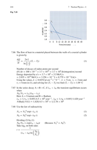
![336 6 Special Theory of Relativity
or
tan θμ
∗
= 1/βcγc (3)
tan θμ = sin θμ
∗
/γc(cos θμ
∗
+ βc/βμ
∗
) = 1/γc
2
βc(1 + 1/β∗
μ) (4)
(Since θμ
∗
= π − θν
∗
) and we have used (2)
But β∗
μ = (mπ
2
− mμ
2
)/(mπ
2
+ mμ
2
) (5)
Substituting (5) in (4) and simplifying
tan θμ = (mπ
2
− m2
μ)/2γ 2
cβcm2
π
6.9 The z-component of velocity is zero; hence the particle must be moving in the
xy =plane. Further, the y-component of velocity is unchanged. This implies
that the Lorentz transformation is to be made along x-axis
cPx = γ (cP
x + βE
) (1)
c2
mβx γ0 = γ (c2
mβ
x γ
+ mβγ
c2
) (2)
βx = 1/21/2
, γ0 = 21/2
, β
x = −1/21/2
, γ
= 21/2
, γ = 1/(1 − β2
)1/2
(3)
Using (4) in (1) and simplifying we get β = 2 × 21/2
/3
6.10 Energy conservation gives
T1 + T2 = Q (1)
Momentum conservation gives
P1 + P2 = 0
or p1
2
= p2
2
T1
2
+ 2T1 m1 = T2
2
+ 2T2 m2 (2)
Solving (1) and (2)
T1 = Q(Q + 2m2)/2(m1 + m2 + Q); T2 = Q(Q + 2m1)/2(m1 + m2 + Q)
6.11 γπ = 1 + Tπ /mπ = 1 + 140/140 = 2
βπ = (γπ
2
− 1)1/2
/γπ = (22
− 1)1/2
/2 = 0.866
By Problem 6.54 , Tμ
∗
= 4.0 MeV therefore
γμ
∗
= 1 + Tμ
∗
/mμ = 1 + (4/106) = 1.038
βμ
∗
= (1.037772
− 1)1/2
/1.0377 = 0.267
γμ = γ γμ
∗
(1 + βπ βμ
∗
cos θ∗
)
γμ(max) = γπ γμ
∗
(1 + βπ βμ
∗
) = 2 × 1.038(1 + 0.866 × 0.267) = 2.556
(Because θ∗
= 0)
Tμ(max) = (γμ(max) − 1)mμ = 165 MeV
Using the formula for optical Doppler effect
Tν(max) = γπ Tν
∗
(1 + βπ ) = 2 × 29.5(1 + 0.866) = 110 MeV
6.12 βc = |p+ + p−|/(E+ + E−)
Using the invariance principle
(total energy)2
− (total momentum)2
= invariant
(E+ + E−)2
− |p+ + p−|2
= (E1
∗
+ E2
∗
)2
− |p1
∗
+ p2
∗
|2
But E1
∗
= E2
∗
since the particles have equal masses. Also by definition of
center of mass, |p1
∗
+ p2
∗
| = 0
Therefore, E1
∗2
= E2
∗2
= 1
4
[E+ + E−)2
− (p+
2
+ p−
2
+ 2 p+ p− cos θ)]
where θ is the angle between e+
− e−
pair](https://image.slidesharecdn.com/1000-solved-problems-in-modern-physics-220626164600-18e7ea67/85/1000-solved-problems-in-modern-physics-pdf-436-320.jpg)
![6.3 Solutions 337
E1
∗
= E2
∗
= (1/4)[(E+
2
− p+
2
+ E−
2
− p−
2
+ 2(E+ E− − p+ p− cos θ)]
E1
∗
= E2
∗
= (1/4)[m2
+ m2
+ 2(E+ E− − p+ p− cos θ)]
= (1/2)(m2
+ E+ E− − p+ p− cos θ)
or E1
∗
= E2
∗
= [1/2(m2
+ E+ E− − p+ p− cos θ)]1/2
6.13 tan θ = sin θ∗
/γc(cos θ∗
+ βc/β1
∗
) = (1/γc) tan θ∗
/2 (1)
(Because βc = β1
∗
)
Also
tan ϕ = (1/γc) tan θ∗
/2 (2)
Where θ∗
and ϕ∗
are the corresponding angles in the CM system
Multiply (1) and (2)
tan θ tan ϕ = (1/γc
2
). tan θ∗
/2. tan ϕ∗
/2
But ϕ∗
= π − θ∗
and for m1 = m2, γc = ((γ + 1)/2)1/2
tan θ tan ϕ = 2/(γ + 1)
In the classical limit, γ → 1 and tan θ tan ϕ = 1
But since tan(θ + ϕ) = (tan θ + tan ϕ)/(1 − tan θ tan ϕ)
tan(ϕ + θ) → ∞
i.e. θ + ϕ = π/2
For γ 1, tan θ tan ϕ 1. For tan(θ + ϕ) to be finite (θ + ϕ) π/2
Hence, for γ 1; θ + ϕ π/2
6.14 The total energy carried by π+
in the rest frame of K+
can be calculated from
Eπ+ = (mK
2
+ mπ
2
− mν
2
)/2mk = 265 MeV (1)
γc = γ ∗
π+ = 265/139.5 = 1.9
and βc = βπ
∗
= (γ ∗2
π+ − 1)1/2
/γ ∗
π+
In the rest frame of pion, the total energy of muon is obtained again by (1)
Eμ+
2
= (mμ+
2
+ mπ+
2
− 0)/2mπ+ = 110 MeV
γμ
∗
= 110/106 = 1.0377
βμ
∗
= (γ ∗2
μ − 1)1/2
/γμ
∗
= 0.267
The Lorentz factor γμ for the muon in the LS is obtained from γμ = γcγ ∗
μ(1 +
β∗
μβc cos θ∗
μ) where θ∗
μ is the emission angle of the muon in the rest frame of
pion. Put θ∗
μ = 0 to obtain γμ(max) and θ∗
μ = 180◦
to obtain γμ(min). The
maximum and minimum kinetic energies are 150 and 55.5 MeV.
6.15 First we find the momenta of three pions by using the formula
P1 = (E2
1 −m2
)1/2
etc, where the total energy, E1 = T1 +m, m = 140 MeV is
the pion mass. We need to find the total momentum of the three particles. Take
the direction of the middle particle as x-axis. Calculate these components as
below:
T1(MeV) = 190, E1 = 330(MeV), P1 = 299 MeV/c,
p1(x) = 276.4 MeV/c, p1(y) = −114 MeV/c
T2 = 321, E2 = 461, P2 = 439, p2(x) = 439, p2(y) = 0
T3 = 58, E3 = 198, P3 = 140, p3(x) = 137, p3(y) = 227
E = 989 MeV,
p(x) = 852.4 MeV/c
P(y) = −84 MeV/c](https://image.slidesharecdn.com/1000-solved-problems-in-modern-physics-220626164600-18e7ea67/85/1000-solved-problems-in-modern-physics-pdf-437-320.jpg)
![338 6 Special Theory of Relativity
Fig. 6.4 Decay of a charged
unstable particle into three
pions
Therefore, P = [
p(x)2
+ (
p(y)2
]1/2
= 856.4 MeV/c
The mass of the particle is given by
M =
*
E
2
−
%
%
p
%
%2
+1/2
= [(989)2
− (856.4)2
]1/2
= 494.7 MeV
It is a K meson
We can find the direction of K meson by calculating the resultant momenta
of the three pions and its orientation with respect to one of the pions.
By the vector addition of p2 and p3 we find the resultant P23 = 576.6 MeV/c
inclined at angle α = 2.84◦
above p2 as in the Fig. 6.4. The angle inclined
between P23 and p1 is ϕ = 2.84 + 22.4 = 25.24◦
.
When p23 is combined with vector p we find that the resultant is inclined at
an angle of 16.7◦
above p1.
6.3.2 Length, Time, Velocity
6.16 L = γ L0 = (1 − β2
)1/2
L0 = (1 − 0.82
)1/2
L0
= 0.6L0
ΔL = L0 − L = 0.4L0
6.17 L = L0/γ = L0/2
γ = 2 → β = (γ 2
− 1)1/2
/γ = (22
− 1)1/2
/2 = 0.866
v = βc = 0.866 × 3 × 108
= 2.448 × 10⁸
ms−1
6.18 β = v/c = 30 km s−1
/3 × 105
km s−1
= 10−4
1/γ = (1 − β2
)1/2
= (1 − 1/2 × β2
)
ΔL = L0 − L = L0 − L0/γ = L0 − L0(1−β2
)1/2
= 1
2
L0β2
= 1/2×6,400×
10−8
km = 3.2 cm
Thus the earth appears to be shrunk by 3.2 cm.
6.19 τ = γ τ0
1.5 × 10−5
= 2.2 × 10⁻⁶
γ
γ = 6.818
β = (γ2
− 1)1/2
/γ = 0.9892
v = 0.9890c](https://image.slidesharecdn.com/1000-solved-problems-in-modern-physics-220626164600-18e7ea67/85/1000-solved-problems-in-modern-physics-pdf-438-320.jpg)
![6.3 Solutions 341
and at the counter C
Ic = IA exp (−2d/γβcτ) (2)
∴ Ic =
I2
B
IA
=
(470)2
1000
= 221
(b) Take logarithm on both sides of (1) and simplify.
τ =
d
γβcln(IA/IB)
(3)
γ = 1 + T/mc2
= 1 + 140/140 = 2.0
β = (γ 2
− 1)1/2
/γ = 0.866
d = 10 m; c = 3 × 10⁸
m/s
ln(IA/IB) = ln(1000/470) = 0.755
Substituting the above values in (3),
τ = 2.55 × 10⁻⁸
s
The accepted value is 2.6 × 10⁻⁸
s
6.36 The stationary object will appear to move with velocity −βc toward the
observer. The object moving with velocity αc toward the stationary object
would appear to have velocity
(αc − βc)/(1 − αβ), as seen by the observer. If these two velocities are to be
equal then (αc − βc)/(1 − αβ) = βc
Cross multiplying and simplifying we get the quadratic equation whose
solution is β = [1 − (1 − α2
)1/2
]/α
6.37
(i) t =
L
βc
(1)
N2 = N1 exp[−t/γ τ] = N1 exp
−
L
γβcτ
(2)
Therefore (2) becomes
exp
*
L
γβcτ
+
= N1/N2
Take logarithm on both sides
L
γβcτ
= ln
N1
N2
But γβ =
γ 2 − 1
Therefore τ = L
ln
N1
N2
√
γ 2−1c
(ii) γ = 1/(1 − β2
)1/2
= 1/(1 − 8/9)1/2
= 3
τ =
200
ln
10,000
8,983
√
32 − 1 × 3 × 108
= 2.2 × 10⁻⁶
s.](https://image.slidesharecdn.com/1000-solved-problems-in-modern-physics-220626164600-18e7ea67/85/1000-solved-problems-in-modern-physics-pdf-441-320.jpg)
![6.3 Solutions 343
6.43 (a) γ = 1 + T/m = 1 + 1, 000/940 = 2.064
β = (γ 2
− 1)1/2
/γ = [(2.064)2
− 1]1/2
/2.064 = 0.87
(b) γ = 1 + 1, 000/0.511 = 1, 958
β = [1, 9582
− 1]1/2
/1, 958 = 0.999973
6.44 (a) There are 6 protons and 6 neutrons in 12
C nucleus.
Δmc2
= [(1.007825 × 6 + 1.008665 × 6 − 12.000] × 931.5
= 92.16 MeV
(b) Δmc2
= [3 × 4.002603 − 12.000] × 931.5
= 7.27 MeV
(c) Δmc2
= [2 × (mn + mp) − mα] × 931.5
= [2 × (1.008665 + 1.007825) − 4.002603] × 931.5
= 28.296 MeV
Total energy required = 3 × 28.296 + 7.27 = 92.16 MeV
which is identical with that in (a)
6.45 c2
p2
= T 2
+ 2T mc2
m = (c2
p2
− T 2
)/2T = (3682
− 2502
)/2 × 250 = 145.85 MeV
Or m = 145.85/0.511 = 285.4 me
The particle is identified as the pion whose actual mass is 273 me
6.46 E0 = m0c2
= (9.1 × 10⁻³¹
kg)(3 × 10⁸
ms−1
)2
= 8.19 × 10⁻¹⁴
J
= (8.19 × 10⁻¹⁴
J)(1 MeV/1.6 × 10−13
J)
= 0.51 MeV
6.47 γ = 1/(1 − β2
)1/2
= 1/(1 − 0.62
)1/2
= 1.25
Energy acquired by electron
T = (γ − 1)mec2
= (1.25 − 1) × 0.51 = 0.1275 MeV
1 eV energy is acquired when an electron (or any singly charged particle) is
accelerated from rest through a P.D of 1 V. Hence the required P.D is 0.1275
Mega volt or 127.5 kV.
6.48 (a) K(relativistic) = (γ − 1)m0c2
(1)
K(classical) = (1/2)m0v2
= (1/2)m0c2
β2
= (1/2)m0c2
(γ 2
− 1)/γ 2
(2)
ΔK
K
=
K(relativistic) − K(Classical)
K(relativistic)
=
γ − 1
2γ
(3)
where we have used (1) and (2)
Putting ΔK/K = 1/100, we find γ = 50/49. Using
β = (γ2
− 1)/γ (4)
we obtain β = 0.199
Or v = 0.199 c
(b) Putting ΔK/K = 10/100 = 1/10 in (3), we find γ = 5/4, Using (4) we
obtain β = 0.6
Or v = 0.6 c](https://image.slidesharecdn.com/1000-solved-problems-in-modern-physics-220626164600-18e7ea67/85/1000-solved-problems-in-modern-physics-pdf-443-320.jpg)
![344 6 Special Theory of Relativity
6.49 T = (γ − 1)m0c2
= [1/(1 − β2
)1/2
− 1]m0c2
= [(1 − β2
)−1/2
− 1]m0c2
= [1 + 1
2
β2
+ 3
8
β4
+ . . . − 1]m0c2
= [1 + 3
4
β2
+ . . .](1
2
m0β2
c2
)
where we have expanded the radical binomially
For v/c 1 or β 1, obviously T m0c2
For small velocities T = m0β2
c2
/2 + small terms = m0v2
/2
6.50 (a) The photon energy Eγ = 1, 240/500 nm = 2.48 eV
= 2.48 × (1.6 × 10−19
) J
= 3.968 × 10⁻¹⁹
J
Effective mass, m = Eγ /c2
= 3.968 × 10⁻¹⁹
/(3 × 108
)2
= 4.4 × 10−36
kg
(b) E = 1,240/0.1 nm = 12,400 eV = 1.984 × 10⁻¹⁵
J
m = 1.984 × 10⁻¹⁵
/(3 × 108
)2
kg = 2.2 × 10⁻³²
kg.
6.51 1amu = 1.66 × 10⁻²⁷
kg
=
(1.66 × 10⁻²⁷
kg)(c2
)
c2
= 1.66 × 10−27
× 2.998 × 108
)2
J/c2
= 1.492 × 10⁻¹⁰
J/c2
= 1.492 × 10⁻¹⁰
J/MeV.MeV/c2
= 1.492 × 10⁻¹⁰
/1.602 × 10−13
MeV/c2
= 931.3 MeV/c2
6.52 Number of Uranium atoms in 1.0 g is
N = N0/A = 6.02 × 10²³
/235 = 2.56 × 10²¹
Number in 5 kg = 2.56 × 1021
× 5,000 = 1.28 × 1025
In each fission ∼ 200 MeV energy is released.
Therefore, total energy released
= 1.28 × 1025
× 200 = 2.56 × 1027
MeV
= (2.56 × 1027
MeV/J)(1.6 × 10−13
J)
= 4 × 10¹⁴
J
6.53 The analysis is similar to that for Compton scattering except for some approx-
imations.
Energy conservation gives
E = E
+ T (1)
From momentum triangle (Fig 6.6)
p 2
= p2
+ pe
2
− 2ppe cos θ (2)
Using c2
p 2
= E 2
− M2
c4
(3)
c2
pe
2
= T 2
+ 2T mc2
(4)
p = γ Mβc (5)
γ = 1/(1 − β)1/2
(6)
Combining (1) – (6) and simplifying and using the fact that mc2
E. we
easily obtain the desired result.](https://image.slidesharecdn.com/1000-solved-problems-in-modern-physics-220626164600-18e7ea67/85/1000-solved-problems-in-modern-physics-pdf-444-320.jpg)
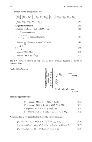
![346 6 Special Theory of Relativity
6.56 TK = [(MD − MK )2
− M2
π ]/2MD = [(1865 − 494)2
− 1402
]/2 × 1865
= 498.67 MeV
PK = (TK
2
+ 2MK TK )1/2
= 861 MeV/c
EK
2
= pK
2
+ mK
2
= (0.861)2
+ (0.494)2
= 0.9853 GeV2
EK = 0.9926 GeV/c
Eπ
2
= pπ
2
+ mπ
2
= (0.861)2
+ (0.140)2
= 0.7609 GeV2
Eπ = 0.8736 GeV
Mx = EK + Eπ = 1.8662 GeV/c2
It is a D0
meson.
6.57 The mass of neutrino is zero. Applying conservation laws of energy and
momentum
Eμ + Eν = mπ c2
(1)
pμ = pν (2)
Multiplying (2) by c and squaring
c2
pμ
2
= c2
pν
2
Or Eμ
2
− mμ
2
c4
= Eν
2
Or Eμ
2
− Eν
2
= mμ
2
c4
(3)
Solve (1) and (3)
γμ = (m2
π + m2
μ)/2mπ mμ
βμ = (1 − 1/γ 2
μ)1/2
= (mπ
2
− mμ
2
)/(mμ
2
+ mμ
2
)
6.58 EB + EC = mAc2
(energy conservation) (1)
PB = PC (momentum conservation) (2)
Or c2
PB
2
= c2
PC
2
(3)
Using the relativistic equations E2
= c2
p2
+ m2
c4
, (3) becomes
EB
2
− mB
2
c4
= EC
2
− mC
2
c4
(4)
Eliminating EC between (1) and (4), and simplifying
EB = (mA
2
+ mB
2
− mC
2
)c2
/2mA (5)
6.59 K+
→ e+
+ π◦
+ νe
The maximum energy of positron will correspond to a situation in which the
neutrino is at rest. In that case the total energy carried by electron will be
Ee(max) = (m2
K +m2
e −m2
π0 )/2mK = (4942
+0.52
+1352
)/2×494 = 228.5MeV
∴ Te(max) = 228 MeV
6.60 Let the incident particle carry momentum p0. As the scattering is symmetrical,
each particle carries kinetic energy T/2 and momentum P after scattering, and
makes an angle θ/2 with the incident direction.
Momentum conservation along the incident direction gives
p0 = p cos θ/2 + p cos θ/2 = 2p cos θ/2 (1)
Or (T 2
+ 2T mc2
)1/2
= 2(T2
/4 + 2T/2mc2
)1/2
cos θ/2 (2)
Squaring (2), and using the identity, cos2
θ/2 = (1 + cos θ)/2
We get the result cos θ = T/(T + 4mc2
)](https://image.slidesharecdn.com/1000-solved-problems-in-modern-physics-220626164600-18e7ea67/85/1000-solved-problems-in-modern-physics-pdf-446-320.jpg)
![6.3 Solutions 347
Fig. 6.7 Symmetrical elastic
collision between identical
particles
6.61 (γ − 1)mc2
= mc2
γ = 2
β = (1 − 1/γ 2
)1/2
=
√
3/2
pe = mγβc
cpe = mc2
γβ = mc2
× 2 ×
√
3/2 = mc2
×
√
3 MeV
pγ = pe =
√
3E0 MeV/c
6.62 For the three particles the energies (total) are equal.
E1 = E2 = E3 (3)
(masses are neglected)
The magnitude of momenta are also equal
p1 = p2 = p3
The momenta represented by the three vectors AC, CB and BA form the closed
Δ ABC.
180◦
− θ = 60◦
Therefore, θ = 120◦
Thus the paths of any two leptons are equally inclined to 120◦
Fig. 6.8 Decay of a muon at
rest into three leptons whose
masses are neglected
6.63 By Problem 6.53, T = 2mc2
β2
cos2
θ/[1 − β2
cos2
θ] (1)
T = 109
eV = 1, 000 MeV
γ = 1 + T/M = 1 + 1, 000/940 = 2.0638
β = [1 − (1/γ 2
)]1/2
= [1 − (1/2.0638)2
]1/2
= 0.875
Using mc2
= 0.511 MeV, β = 0.875 and θ = 3◦
in (1),
We find T = 3.3 MeV](https://image.slidesharecdn.com/1000-solved-problems-in-modern-physics-220626164600-18e7ea67/85/1000-solved-problems-in-modern-physics-pdf-447-320.jpg)
![348 6 Special Theory of Relativity
6.64 (a) π+
→ μ+
+ νμ
T = Q(Q + 2mν)/2(mμ + mν + Q) = (mπ − mμ)2
/2mπ
(Q = mπ − mμ − mν = mπ − mμ and mν = 0)
mμ = 206.9me = 206.9 × 0.511 = 105.7 MeV
Therefore,
Tμ = 4.12 = (mπ − 105.7)2
/2mπ
Solving for mπ
mπ = 141.39 MeV/c2
= 141.39/0.511me
= 276.7me
(b) μ+
→ e+
+ νe + νμ
Tmax for electron is obtained when νe and νμ fly together in opposite direc-
tion. Thus, the three-body problem is reduced to a two-body one.
mμc2
= 206.9 × 0.511 = 105.72 MeV
Q = 105.72 − 0.51 = 105.21 MeV
Te(max) = Q2
/2(me + Q) = (105.72)2
/2(0.51 + 105.72) = 52.6 MeV
6.65 Q = 938.2 + 1,875.5 − (939.5 + 135.0) − 2.2 = 1,737 MeV
Tπ = Q(Q + 2mn)/2(Q + mπ + mn)
= 1,737(1,737 + 2 × 939.5)/2(1, 737 + 135 + 939.5) = 1, 117 MeV
Total energy Eπ = 1, 117 + 135 = 1, 252 MeV
6.66 M2
= m1
2
+ m2
2
+ 2(E1 E2 − P1 P2 cos θ) (1)
m1 = 966 me = 966 × 0.511 MeV = 493.6 MeV (2)
m2 = 273 me = 273 × 0.511 MeV = 139.5 MeV (3)
p1 = 394 MeV, p2 = 254 MeV (4)
E1 = (p1
2
+ m1
2
)1/2
= [(394)2
+ (93.6)2
]1/2
= 631.6 (5)
E2 = (p2
2
+ m2
2
)1/2
= [(254)2
+ (139.5)2
]1/2
= 289.5 (6)
cos θ = cos 154◦
= −0.898 (7)
Using (2) to (7) in (1), M = 899.4 MeV
6.67 Using the results of Problem 6.60, the angle between the outgoing particles
after the collision is given by
cos θ = T/(T + 4M)
Here T = 940 MeV = M
Therefore, cos θ = 0.2 → θ = 78.46◦
6.68 Using the invariance, E2
− |
p|2
= E∗2
E∗2
= (E + Ef)2
− (p2
+ p2
f + 2ppf cos θ)
= (E + Ef)2
− (E2
− M2
+ E2
f − M2
+ 2ppf cos θ
= 2M2
+ 2(E Ef − p.pf)
(a) For parallel momenta, θ = 0, p.pf = +ppf
(b) For anti-parallel momenta θ = π, p.pf = −ppf
(c) For orthogonal momenta θ = π/2, p.pf = 0
6.69 By problem 6.13 it is sufficient to show that tan θ tan ϕ = 2/(γ + 1)
p = γβm = (γ 2
− 1)1/2
m](https://image.slidesharecdn.com/1000-solved-problems-in-modern-physics-220626164600-18e7ea67/85/1000-solved-problems-in-modern-physics-pdf-448-320.jpg)
![6.3 Solutions 349
Therefore, γ = [1 + (p/m)2
]1/2
= [1 + (5/0.938)2
]1/2
= 5.41
tan θ tan ϕ = tan 82◦
tan 2◦
30
= 7.115 × 0.04366 = 0.3106
2/(γ + 1) = 2/(5.41 + 1) = 0.3120
Hence the event is consistent with elastic scattering.
6.70 Let p, pe, pN be the momentum of the incident electron, scattered electron
and recoil nucleus, respectively. From the momentum triangle, Fig. 6.9.
pN
2
= pe
2
+ p2
− 2ppe cos θ = EN
2
+ 2EN M (1)
where we have put c = 1
From energy conservation
EN + Ee = E (2)
As
Ee ≈ pe (3)
E ≈ P (4)
(2) Can be written as
EN + pe = E (5)
Combiining (1), (3), (4) and (5), we get
EN = E2
(1 − cos θ)/M[1 + E/M(1 − cos θ)]
Restoring c2
, we get the desired result.
Fig. 6.9 Momentum triangle
6.71 Use the result of Problem 6.53,
T = 2mc2
β2
cos2
ϕ/(1 − β2
cos2
ϕ) (1)
Put c = 1, T = E − m (2)
P = Mβγ = Mβ/(1 − β2
)1/2
whence β2
= P2
/(P2
+ M2
) (3)
Use (2) and (3) in (1) and simplify to get the desired result.
6.72 The formula for the recoil energy of electron in Compton scattering is
T = (E2
/mc2
)(1 − cos θ)/[1 + α(1 − cos θ)]
Here neutrinos are assumed to be massless, so that the same formula which
is based on relativistic kinematics can be used.
The maximum recoil energy will occur when the neutrino is scattered
back, that is θ = 180◦
. Substituting E = 2 GeV for the incident neutrino
energy, mc2
= 0.511 MeV = 0.511 × 10⁻³
GeV, and α = E/mc2
=
2/0.511×10−3
= 3,914, we find the maximum energy transferred to electron
is 1.9997 GeV. The maximum momentum transfer
pmax = (T2
max + 2 mec2
.Tmax)1/2
= 2.0437 GeV/c](https://image.slidesharecdn.com/1000-solved-problems-in-modern-physics-220626164600-18e7ea67/85/1000-solved-problems-in-modern-physics-pdf-449-320.jpg)
![350 6 Special Theory of Relativity
6.73 Expressing θ in terms of θ∗
tan θ = sin θ∗
/γc(cos θ∗
+ βc/β∗
) (1)
Differentiating with respect to θ∗
and setting ∂ tan θ/∂θ∗
= 0, gives
cos θ∗
= −β∗
/βc (2)
And sin θ∗
= (β2
c − β∗2
)1/2
/βc (3)
Using (2) and (3) in (1), and the equations
β∗2
γ ∗2
= γ ∗2
− 1 (4)
βc
2
γc
2
= γc
2
− 1 (5)
as well as
m1β∗
γ ∗
= m2βcγc (momentum conservation in the CMS) (6)
and simplifying, we get
tan θmax = [m2
2
/(m1
2
− m2
2
)]1/2
6.74 Let P1 be the electron four-momentum before the collision and P2 the final
four-momentum. If Q is the four-momrntum transfer then the conservation of
energy and momentum requires that
Q = P2 − P1 (1)
and Q2
= Q.Q = P2
2
+ P1
2
− 2P1P2 (2)
But P = (p, E/c) (3)
P2
c2
= E2
− p.pc2
= me
2
c4
(4)
For stationary electron, the initial four-momrntum is
P1 = (0, mec) (5)
and final four-momentum
P2 = (p2, mec + ν/c) (6)
Therefore
P1.P2 = mec(mec + ν/c) (7)
Substituting (7) in (2) and using (4)
Q2
= 2me
2
c4
− 2mec(mec + ν/c)
= −2 meν
6.75 (a) As the collision is elastic the total initial energy = total final energy.
E + Ee = E
+ Ee
(1)
But p
= p (2)
∴ E
= E (3)
It follows that E
e = Ee (4)
Consequently pe
= pe (5)
Momentum conservation gives
p − pe = −p
+ pe
(6)](https://image.slidesharecdn.com/1000-solved-problems-in-modern-physics-220626164600-18e7ea67/85/1000-solved-problems-in-modern-physics-pdf-450-320.jpg)
![6.3 Solutions 351
Because of (2) and (5)
p
e = p = E/c
(b) β = v/c = (1 − 1/γ 2
)1/2
= (1 − m2
/Ee
2
)1/2
= (1 − m2
/(pe
2
+ m2
))1/2
= (pe
2
/(pe
2
+ m2
))1/2
= (1 + (mc
2
/E)2
)−1/2
where Pe = E and c = 1.
6.3.4 Invariance Principle
6.76 Referring to Fig. 7.8, let Pγ and Pγ
be the four-momentum vectors of photon
before and after the scattering, respectively, Pe and Pe
the four vectors of
electron before and after scattering respectively. Form the scalar product of
the four-vector of the photon and the four-vector of photon + electron. Since
this scalar product is invariant.
Pγ .(Pγ + Pe) = Pγ
.(Pγ
+ Pe
) (1)
Further, total four-momentum is conserved.
Pγ + Pe = Pγ
+ Pe
(2)
Now, Pγ = [hν, 0, 0, ihν] (3)
Pe = [0, 0, 0, imc] (4)
Pγ
= [h ν
cos θ, h ν
sin θ, 0, ihν]
where m is the rest mass of the electron.
Using (1) to (4)
[hν, 0, 0, ihν].[hν, 0, 0, i(hν + mc2
)]
= [hν
cos θ, hν
sin θ, 0, ihν].[hν, 0, 0, i(hν + mc2
)]
Therefore, h2
ν2
− hν(hν + mc2
) = h2
νν
cos θ − hν
(hν + mc2
)
Simplifying
hν
ν(1 − cos θ) = mc2
(ν − ν
)
Or h/mc(1 − cos θ) = c(1/ν
− 1/ν) = λ
− λ
Or Δλ = λ
− λ = (h/mc)(1 − cos θ)
This is the well known formula for Compton shift in wavelength (formula
7.37).
6.77 Let the initial and final four momenta of the electron be Pi = (Ei/c, pi) and
Pf = (Ef, pf), respectively. The squared four-momentum transfer is defined by
Q2
= (Pi − Pf)2
= −2m2
c2
+
2Ei Ef
c2
− 2Pi · Pf
However, Ei = Ef = E and |pi| = |pf| = E/c; so neglecting the electron
mass
Q2
= 2E2
(1 − cos θ)/c2](https://image.slidesharecdn.com/1000-solved-problems-in-modern-physics-220626164600-18e7ea67/85/1000-solved-problems-in-modern-physics-pdf-451-320.jpg)
![352 6 Special Theory of Relativity
6.78
1
2
(M2
− m1
2
− m2
2
) = E1 E2 − p1 p2 cos θ
θ = 900
P± = 530 MeV/c
E± = (P2
± + mπ
2
)1/2
= 548
2 × 5482
+ 2 × 1402
= M2
M = 800 MeV/c
It is a ρ meson.
Fig. 6.10
6.79 Using the invariance of squared four-momentum before and after the decay
Ei
2
− Pi
2
= Ef
2
− |pf|2
M2
= (E1 + E2)2
− (p1
2
+ p2
2
+ 2p1 p2 cos θ)
= (E1
2
− p1
2
) + (E2
2
− p2
2
) + 2(E1 E2 − p1 p2 cos θ)
= m1
2
+ m2
2
+ 2(E1 E2 − p1 p2 cos θ)
Or E1 E2 − p1 p2 cos θ =
1
2
(M2
− m1
2
− m2
2
) = Invariant
6.80 s + t + u = (1/c2
)[(PA + PB)2
+ (PA − PC )2
+ (PA − PD)2
]
= (1/c2
)[3PA
2
+ PB
2
+ PC
2
+ PD
2
+ 2PA(PB − PC − PD)] (1)
From four-momentum conservation, PA + PB = PC + PD (2)
(1) becomes (s + t + u)c2
= (3mA
2
+ mB
2
+ mC
2
+ mD
2
) − 2PA
2
Using PA = mAc, PB = mBc, PC = mC c and PD = mDc
(s + t + u)c2
= (mA
2
+ mB
2
+ mC
2
+ mD
2
)c2
Or s + t + u =
i=A,B,C,D
m2
i
6.81 t = (PA − PC )2
/c2
= (1/c2
)(PA
2
+ PC
2
− 2PA PC )
= (1/c2
)[mA
2
c2
+ mC
2
c2
− 2(EA EC /c2
− PA.PC )]
For elastic scattering A ≡ C. Thus EA = EC and |PA| = |PC | = p
So that PA.PC = p2
cos θ.
c2
t = 2mA
2
c2
− 2(EA
2
/c2
− p2
cos θ)
But EA
2
= c2
p2
+ mA
2
c4
Therefore, t = −2p2
(1 − cos θ)/c2
6.82 sin ϕ/2 = mπ c2
/2(E1 E2)1/2
(see Prob. 6.103 and 6.104)
Minimum angle is ϕmin = 2/γ](https://image.slidesharecdn.com/1000-solved-problems-in-modern-physics-220626164600-18e7ea67/85/1000-solved-problems-in-modern-physics-pdf-452-320.jpg)
![356 6 Special Theory of Relativity
6.91 (a) λ/λ
= [(1 + β)/(1 − β)]1/2
= 656/434 = 1.5115
v = βc = 1.17 × 10⁸
ms−1
(b) the nebula is receding
6.92 λ/λ
= [(1 + β)/(1 − β)]1/2
= (1 + β)1/2
(1 − β)−1/2
≈ (1 + β/2 + . . .)(1 + β/2 − . . .)
= 1 + β + . . . (neglecting higher order terms)
Δλ/λ
= (λ/λ
) − 1 = β = v/c
6.93 λ/λ
= [(1 + β)/(1 − β)]1/2
= 670/525
β = 0.239
v = βc = 0.239 × 3 × 108
= 7.17 × 10⁷
ms−1
= 7.17 × 10⁴
kms−1
This speed exceeds the escape velocity. Hence the explanation is not valid.
6.94 λ
= λ[(1 − β)/(1 + β)]1/2
= 589.3[(1 − 0.21)/(1 + 0.21)]1/2
= 476.2 nm
The color is blue
6.95 The source velocity is perpendicular to the line of sight. θ = 90◦
,
ν
= νγ
λ = γ λ
γ = 1/(1 − β2
)1/2
= 1/(1 − 0.052
)1/2
= 1.00125
Δλ = λ − λ
= λ
(γ − 1) = 589(1.00125 − 1)
= 0.736 nm = 7.36 Å
6.96 Let the electron recoil at angle ϕ with momentum p, and neutrino get scat-
tered with energy E
and momentum p
.
Energy conservation gives
E0 + m = E + E
(1)
From the momentum triangle
p 2
= p0
2
+ p2
− 2p0 p cos ϕ (2)
We can write p
= E
, p = E, p0 = E0, so that (2) becomes
E 2
= E0
2
+ E2
− 2E0 E cos ϕ (3)
Fig. 6.13 Collision of an energetic neutrino with a stationary electron](https://image.slidesharecdn.com/1000-solved-problems-in-modern-physics-220626164600-18e7ea67/85/1000-solved-problems-in-modern-physics-pdf-456-320.jpg)
![6.3 Solutions 357
From (1) we have
E 2
= (E0 − E + m)2
(4)
Comparing (3) and (4) and simplifying
cos ϕ = 1 − m(E0 − E − m)/E0 E ≈ 1 − m(E0 − E)/E0 E (5)
where we have neglected m in comparison with E0 − E.
For small angle, (5) becomes ϕ = [2m(E0 − E)/E0 E]1/2
(6)
For E0 = 2 GeV, E = 0.5 GeV, m = 0.51 × 10⁻³
GeV
ϕ = 0.039 radians = 2.24◦
6.97 Let the mass of the primary particle be M, and that of secondary particles m1
and m2. Let the total energy of the secondary particles in the LS be E1 and
E2, and momenta p1 and p2. Using the invariance of (total energy)2
− (total
momentum)2
M2
= (E1 + E2)2
− (p1
2
+ p2
2
+ 2p1 p2 cos θ)
= E1
2
− p1
2
+ E2
2
− p2
2
+ 2(E2
1 − p1
2
cos θ)
= m1
2
+ m2
2
+ 2(E1
2
− p1
2
cos θ) (Since E1 = E2, p1 = p2)
= 2m1
2
+ 2(m1
2
+ p1
2
− p1
2
cos θ)
= 4m1
2
+ 4p1
2
sin2
θ/2
= 4(140)2
+ 4(300)2
sin2
35◦
= 196,836
M = 444 MeV/c2
6.98 Consider one of the two γ -rays. From Lorentz transformation
cpx = γc(cpx
∗
+ βc E∗
)
where the energy and momentum refer to one of the two γ -rays and the
subscript C refers to π0
. Starred quantities refer to the rest system of π0
.
cp cos θ = γ (cp∗
cos θ∗
+ βE∗
)
where we have dropped off the subscript C. But for γ -rays cp∗
= E∗
and
cp = E, and because the two γ -rays share equal energy in the CMS, E∗
=
mc2
/2, where m is the rest mass of π◦
.
Therefore cp cos θ = (γ mc2
/2)(β + cos θ∗
) (1)
Also, E = γ (E∗
+ βcp∗
x ) = γ (E∗
+ βcp∗
cos θ∗
)
or
cp = E = (γ mc2
/2)(1 + β cos θ∗
) (2)
When θ∗
= 0
Emax =
1
2
Eπ◦ (1 + β) (3)
When θ∗
= π
Emin =
1
2
Eπ◦ (1 − β) (4)](https://image.slidesharecdn.com/1000-solved-problems-in-modern-physics-220626164600-18e7ea67/85/1000-solved-problems-in-modern-physics-pdf-457-320.jpg)
![6.3 Solutions 361
6.103 The angle between the two γ -rays in the LS can be found fom the formula
m2
c4
= m1
2
c4
+ m2
2
c4
+ 2(E1 E2 − c2
p1 p2 cos ϕ)
Putting m1 = m2 = 0, cp1 = E1, cp2 = E2
m2
c4
= 2E1 E2(1 − cos ϕ) = 4E1 E2 sin2
(ϕ/2)
sin (ϕ/2) = mc2
/2(E1 E2)1/2
(15)
6.104 For small angle ϕ,
ϕ = mc2
/(E1 E2)1/2
(16)
Set E2 = γ mc2
− E1
ϕ = mc2
/[E1(γ mc2
− E1)]1/2
(17)
For minimum angle d ϕ/dE1 = 0. This gives E1 = γ mc2
/2.
Using this value of E1 in (17), we obtain
ϕmin = 2/γ (18)
Measurement of ϕmin affords the determination of Eπ via γ .
ϕmin = 2mc2
/Eπ
6.105 E1 + E2 = E (energy conservation) (1)
p1 + p2 = p (momentum conservation) (2)
Taking the scalar product
(p1 + p2).(p1 + p2) = p.p
or
p1
2
+ p2
2
+ 2p1 p2 cos θ = p2
(3)
Using c = 1, Eq. (3) becomes
E1
2
+ E2
2
+ 2E1 E2 cos θ = E2
− m2
(4)
Let E2/E1 = D, (5)
the disparity factor. Then (1) becomes
E1(D + 1) = E (6)
Combining (4), (5) and (6)
2DE2
(1 − cos θ) = m2
Or sin θ/2 = [m/2E][
√
D + 1/
√
D]
For small θ,
θ = [m/E][
√
D + 1
√
D]](https://image.slidesharecdn.com/1000-solved-problems-in-modern-physics-220626164600-18e7ea67/85/1000-solved-problems-in-modern-physics-pdf-461-320.jpg)
![362 6 Special Theory of Relativity
The minimum angle is found by setting dθ/dD = 0
This gives us D = 1, that is E1 = E2 = E/2.
θmin = 2mc2
/E
The Lorentz transformation of angles gives us the relation
E = [m γ/2][1 + β cos θ∗
)
We need to consider one of the photons in the forward hemisphere. The
fraction of photons emitted in the CMS (rest frame of π0
) within the angle θ∗
is (1 − cos θ∗
). This fraction is 1/2 for θ∗
= 600
, that is cos θ∗
= 1/2. When
one photon goes at θ∗
= 600
, the other photon will go at θ∗
= 1200
with the
direction of flight of π0
. Hence cos θ∗
= −1/2 for the second photon. The
disparity factor
D = E2/E1 = (1 + β/2)/(1 − β/2) = (2 + β)/(2 − β).
For relativistic pions β = 1 Hence D 1.
A quarter of pions will be emitted within an angle θ∗
= 41.40
, that is
cos θ∗
= 0.75. In this case
D = (1 + 3β/4)/(1 − 3β/4)
And the previous argument gives us D 7
6.106 First find E∗
the total energy available in the CMS
E∗2
= (Eπ + mp)2
− P2
π ≈ (Pπ + mp)2
− Pπ
2
(Because Eπ mπ )
E∗
= 4.436 GeV
Total energy carried by K∗
in the CMS
Ek
∗
= (E∗2
+ mk
∗2
− mγ 0 )/2E∗
= 1.942 GeV
γK
∗
= EK
∗
/mK
∗
= 1.942/0.89 = 2.18
βK
∗
= 0.8888
γc = (γ + ν)/(1 + 2γ ν + ν2
)1/2
γ = 10/0.14 = 71.4
ν = m2/m1 = 0.940/0.140 = 6.71
γc = 2.466, βc = 0.9141
tan θ = sin θ∗
/(cos θ∗
+ βc/β∗
) (1)
Differentiate with respect to θ∗
and set
∂ tan θ/∂θ∗
= 0.This gives cos θ∗
= −β∗
/βc
cos θ∗
= −0.8888/0.9141 = −0.9723
θ∗
= 166.50
Using the values of θ∗
, γc, and the ratio βc/β∗
in (1) we find θm = 59.3◦](https://image.slidesharecdn.com/1000-solved-problems-in-modern-physics-220626164600-18e7ea67/85/1000-solved-problems-in-modern-physics-pdf-462-320.jpg)
![6.3 Solutions 363
6.107 (a), (b) In the CMS, m2 will move with the velocity βc in a direction opposite
to that of m1. By definition, the total momentum in the CMS before and after
the collision is zero. In natural units c = 1.
m1 γ ∗
β∗
= m2 γc βc (1)
Squaring (1) and expressing the velocities in terms of Lorentz factors
m1
2
(γ ∗2
− 1) = m2
2
(γc
2
− 1) (2)
Using the invariance
(ΣE)2
− |ΣP|2
= (ΣE∗
)2
− |ΣP∗
|2
= (ΣE∗
)2
(3)
(because
P∗
= 0, in the CMS)
(m1 γ + m2)2
− m1
2
(γ 2
− 1) = (m1 γ ∗
+ m2 γc)2
(4)
Combining (2) and (4) and calling v = m2/m1
γc = (γ + ν)/(1 + 2γ ν + ν2
)1/2
(5)
γ ∗
= (γ + 1/ν)/(1 + 2γ/ν + 1/ν2
)1/2
(6)
For the special case, m1 = m2, as in the P–P collision
γc = γ ∗
= [(γ + 1)/2]1/2
(7)
In addition if γ 1
γc ≈ (γ/2)1/2
(8)
(c), (d)
The Lorentz transformations are
P cos θ = γc(p∗
cos θ∗
+ E∗
) (9)
P sin θ = p∗
sin θ∗
(10)
Dividing (10) by (9)
tan θ = p∗
sin θ∗
/γc(p∗
cos θ∗
+ βc E∗
) = sin θ∗
/γc(cos θ∗
+ βc/β∗
) (11)
(because p∗
/E∗
= β∗
)
From the inverse transformation
P∗
cos θ∗
= γc(P cos θ − βc E) (12)
and (10) we get
tan θ∗
= sin θ/γc(cos θ − βc/β) (13)
6.108 At the right angle to the direction of source velocity the Doppler shift in
wavelength is calculated from
ν
= γ ν or λ
= λ/γ
where γ is the Lorentz factor of the carbon atoms and T is the kinetic energy
of carbon and Mc2
is the approximate rest mass energy, the quantity](https://image.slidesharecdn.com/1000-solved-problems-in-modern-physics-220626164600-18e7ea67/85/1000-solved-problems-in-modern-physics-pdf-463-320.jpg)
![2
3
= 0.816
The speed at which the rod is moving is v = βc = 0.816 c
6.3.6 Threshold of Particle Production
6.113 For the production reaction
m1 + m2 → m3 + m4
The threshold energy for m1 when m2 is at rest is
T1 = [(m3 + m4)2
− (m1 + m2)2
]/2m2
In the given reaction we can put
m3 + m4 = 4M, m1 = m2 = M
T1 = 6M or T1 = 6Mc2
6.114 Here m1 = 0, m2 = m, (m3 + m4) = 3m
T1 = 4mc2
6.115 If m1 is the projectile mass, m2 target mass, and m3 + m4 + m5, the mass of
product particles. The threshold is given by formula
T1 = [(m3 + m4 + m5)2
− (m1 + m2)2
]/2m2
= [(940 + 940 + 140)2
− (940 + 940)2
]/2 × 940
= 290.4 MeV
The threshold energy is thus slightly greater than twice the rest-mass
energy of pion (140 MeV). Non-relativistically, the result would be 280 MeV,
that is double the rest mass energy of Pion. The extra energy of 10 MeV is to
be regarded as relativistic correction
6.116 Use the invariance of E2
− P2
= E∗2
− P∗2
= E∗2
− 0 = E∗2
E∗2
= (4m)2
= (T + m + m + 0.025)2
− (P1 − 0.218)2
Putting m = 0.938, P1 = (T 2
+ 2T m)1/2
and
solving for T , we find that T (threshold) = 4.3 GeV
6.117 Tthreshold = [(m3 + m4)2
− (m1 + m2)2
]/2m2
= [(0.89 + 1.11)2
− (0 + 0.94)2
]/2 × 0.94
= 3.12 GeV](https://image.slidesharecdn.com/1000-solved-problems-in-modern-physics-220626164600-18e7ea67/85/1000-solved-problems-in-modern-physics-pdf-466-320.jpg)
![366 6 Special Theory of Relativity
6.118 Tthreshold = [(mp + mp + mp)2
− (mp + mp)2
]/2mp by Eq. (6.53)
mp = 1,837 me = 1,837 × 0.00.00051 GeV = 0.937 GeV
M = 273 × 0.00051 GeV = 0.137 GeV
Using the above values we find Tthreshold = 0.167 GeV
6.119 Tthreshold = (mk + mΛ)2
− (mp + mp)2
/2mp
mk = 0.498 GeV, mΛ = 1.115 GeV, mπ = 0.140 GeV, mp = 0.938 GeV
Using these values, we find Tthreshold = 0.767 GeV = 767 MeV
Note that when pions are used as bombarding particles the threshold for
strange particle production is lowered then in N–N collisions. However, first
a beam of pions must be produced in N–N collisions.
6.120 Consider the reaction P + P → P + P + nπ
Tthreshold = [(mp + mp + nmπ )2
− (mp + mp)2
]/2mp
Simplifying we get the desired result
6.121 Tthreshold = [(mp + mπ0)2
− (mp + 0)2
]/2mp
Using mp = 940 MeV and mπ0 = 135 MeV, we
find Tthreshold = 145 MeV
Note that the threshold energy for pion production in collision with gamma
rays is only half of that for N–N collisions. But the cross-section is down by
two orders of magnitude as the interaction is electromagnetic.
6.122 Tthreshold = [(mΞ− + mk + mk0)2
− (mπ− + mp)2
]/2mp
= [(1,321 + 494 + 498)2
− (140 + 938)2
]/2 × 938
= 2,233 MeV
Note that for Ξ production, the threshold is much higher than that for
−
production as it has to be produced in association with two other strange
particles (see Chaps.9 and 10).
6.123 Using the invariance, E2
− |
p|2
= E∗2
− |
p∗
|2
At threshold: (E + Mp)2
− Eν
2
= (Mp + Mμ + Mw)2
− 0
(5 + 0.938)2
− 52
= (0.938 + 0.106 + Mw)2
Mw = 2.16 GeV
Since the reaction does not proceed, Mw 2.16 GeV
6.124 Tthr = [(mp + mΛ + mk)2
− (2mp)2
]/2mp
= [(0.938 + 1.115 + 0.494)2
− (2 × 0.938)2
]/2 × 0.938
= 1.58 GeV](https://image.slidesharecdn.com/1000-solved-problems-in-modern-physics-220626164600-18e7ea67/85/1000-solved-problems-in-modern-physics-pdf-467-320.jpg)
![6.3 Solutions 367
6.125 Tthr = [(mk0 + mk + mΩ−)2
− (mk− + mp)2
]/2mk−
= [(0.498 + 0.494 + 1.675)2
− (0.494 + 0.938)2
]/2 × 0.938 = 2.7 GeV
Minimum momentum pK− = (T 2
+ 2T m)1/2
= (2.72
+ 2 × 2.7 ×
0.494)1/2
= 3.15 GeV/c
Pthr = 3.15 GeV/c
EK = 2.7 + 0.494 = 3.194 GeV
γK = Ek/mk = 3.194/0.494 = 6.46
γc = (γ + m2/m1)/[1 + 2γ m2/m1 + (m2/m1)2
]1/2
m2/m1 = 938/494 = 1.9
γc = (6.46 + 1.9)/(1 + 2 × 6.46 × 1.9 + 1.92
)1/2
= 1.61
γΩ = γc = 1.61; βΩ = (γ 2
Ω − 1)1/2
/γΩ = 0.79
Proper time t0 = d/v = d/βc
Observed time t = γ t0 = γ d/βc = 1.61 × 0.03/0.79 × 3 × 108
=
2 × 10⁻¹⁰
s
Probability that Ω−
will travel 3 cm before decay.
= exp(−t/τ)
= exp(−2 × 10⁻¹⁰
/1.3 × 10−10
)
= 0.21
6.126 TF(max)p = (9/32π2
)2/3
4π2
(2
c2
/2mpc2
r2
0 )(Z/A)2/3
R = r0 A1/3
r0 = R/A1/3
= 5.17/(63)1/3
= 1.3 fm
TF(max)p = (9/32π2
)2/3
× 4π2
(197 MeV − fm)2
(29/63)2/3
/2
× 938 × (1.3)2
= 26.886 MeV
PF(max) = (T2
+ 2T m)1/2
= [(26.886)2
+ 2 × 26.886 × 938]1/2
= 226.2 MeV/c
E2
− (p1 + p2)2
= E∗2
(maximum energy will be available when p1 and
p2 are antiparallel)
E∗
= [(938 + 160 + 938 + 27)2
− (570.4 − 226.2)2
]1/2
= 2034 MeV
md + mπ = 938 + 939 − 2.2 + 139.5 = 2, 014 MeV
As the energy available in the CMS is in excess of the required energy, we
do expect the pions to be produced.](https://image.slidesharecdn.com/1000-solved-problems-in-modern-physics-220626164600-18e7ea67/85/1000-solved-problems-in-modern-physics-pdf-468-320.jpg)
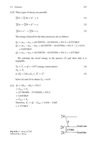
![372 7 Nuclear Physics – I
Fig. 7.3 Concept of
differential cross-section
The unit of σ is a Barn (B). 1 Barn = 10−24
cm2
, 1mB = 10−27
cm2
and 1 μB =
10−30
cm2
. The unit of σ(θ, ϕ) is Barn/Steradian, where steradian (sr) is the unit of
solid angle.
Relation between the differential cross-sections in the LS and CMS
σ(θ) =
(1 + γ 2
+ 2γ cos θ∗
)
3
2
|1 + γ cos θ∗|
σ(θ∗
) (7.11)
where γ = m1/m2
Note that the total cross-section is the same for both LS and CMS because the
occurrence of the total number of collisions is independent of the description of the
process.
Geometric cross-section
σg = π R2
(7.12)
This is the projected area of a sphere of radius R.
Rutherford Scattering
σ (θ) = [1.295(zZ/T )2
/ sin4
(θ/2)] mb/sr (7.13)
σ(θ
, θ
= (π/4)R0
2
[cot2
(θ
/2) − cot2
(θ
/2)] (7.14)
represents the cross-section for particles to be scattered between angles θ
and θ
R0 (fm) = 1.44zZ/T 0(MeV) (7.15)](https://image.slidesharecdn.com/1000-solved-problems-in-modern-physics-220626164600-18e7ea67/85/1000-solved-problems-in-modern-physics-pdf-473-320.jpg)
![7.1 Basic Concepts and Formulae 373
Fig. 7.4 Rutherford
scattering
R0 is also the minimum distance of approach in head-on collision for positively
charged particles of energy below Coulomb barrier (Fig. 7.4).
Impact parameter (b) and scattering angle (θ)
tan (θ/2) = R0/2b (7.16)
Minimum distance of approach
R0
2
1 +
1 +
4b2
R2
0
1/2
'
= (R0/2)[1 + cosec (θ/2)] (7.17)
Multiple scattering angle
The root mean square angle of multiple scattering
√
Θ2
= k
√
t ze/pv (7.18)
where k is the scattering constant
k = [8π N Z2
e2
ln(bmax/bmin)]1/2
t=thickness, N=number of atoms/cm3
, Ze and ze are the charge of nuclei of medium
and projectile, pv is momentum times the velocity of the incident particle. For pho-
tographic emulsions, ln(bmax/bmin) is of the order of 10.
Cross-section and mean free path
If n is the number of atoms/cm3
, then the macroscopic cross-section
Σ = n σ (cm−1
) (7.19)
And mean free path
λ = 1/Σ (7.20)
Also, n = N0 ρ/A (7.21)
where N0 =Avagadro’s number, ρ =density, A the atomic weight.](https://image.slidesharecdn.com/1000-solved-problems-in-modern-physics-220626164600-18e7ea67/85/1000-solved-problems-in-modern-physics-pdf-474-320.jpg)
![374 7 Nuclear Physics – I
Ionization
Bethe’s quantum mechanical formula
− dE/dx = (4π z2
e4
n/mv2
)[ln (2mv2
/I) − ln(1 − β2
) − β2
] (7.22)
where n =number of electrons/cm3
, I =ionization potential, v = β c is the particle
velocity and ze is its charge, m is the mass of electron
Note that −dE/dx is independent of the mass of the incident particle (Fig. 7.5).
Fig. 7.5 Ionization
(−dE/dx) versus particle
energy
Range–Energy-relation
E = kz2n
M1−n
Rn
(7.23)
where k and n are empirical constants which depend on the nature of the absorber,
M is the mass of the particle in terms of proton mass.
If two particles of mass M1 and M2 and atomic number z1 and z2 enter the
absorber with the same velocity then the ratio of their ranges
R1/R2 = (M1/M2)(z2
2
/z1
2
) (7.24)
Range in air – Geiger’s rule
R = const. v3
R = 0.32 E3/2
(alphas in air) (7.25)
Valid for 4–10 MeV α particles. R is in cm and E in MeV
The Bragg–Kleeman rule
If R1, ρ1 and A1 are the range, density and atomic weight in medium 1, the corre-
sponding quantities R2, ρ2 and A2 in medium 2, then
R2/R1 = (ρ1 / ρ2) (A2/A1)1/2
(7.26)](https://image.slidesharecdn.com/1000-solved-problems-in-modern-physics-220626164600-18e7ea67/85/1000-solved-problems-in-modern-physics-pdf-475-320.jpg)
![376 7 Nuclear Physics – I
Motion of a charged particle in a magnetic field
Centripetal force = Magnetic force
mv2
/ρ = qvB (7.30)
Momentum P(GeV/c) = 0.3 Bρ (7.31)
ρ is in meters and B is in Tesla
1 T = 10 k G
Cerenkov radiation
Electromagnetic radiation is emitted when a charged particle on passing through
a medium with a velocity v = βc which exceeds the phase velocity of light c/n,
where n is the index of refraction, the radiation is instantaneous and possesses a
sharply pronounced spatial symmetry.
The radiation is soft and is mostly emitted in the blue part of the spectrum. The
radiation is emitted on a conical surface BDA, as in Fig. 7.7
cos θ = 1/ β n (7.32)
Fig. 7.7 Cerenkov radiation
The threshold velocity
β (thresh) = 1/n (7.33)
The number of photons radiated in the interval dE = h dν by a particle of charge
ze in track length dx is given by
d2
Nγ /dx dE = (α z2
/c) [1 − (1/β2
n2
)] (7.34)
Threshold Cerenkov counters can be used to discriminate between two relativis-
tic particles of the same momentum p and different masses m1 and m2, if the heavier
particle (m2) is just below the threshold. In that case
sin2
θ1 ≈ (m2
2
− m1
2
)/p2
(7.35)](https://image.slidesharecdn.com/1000-solved-problems-in-modern-physics-220626164600-18e7ea67/85/1000-solved-problems-in-modern-physics-pdf-477-320.jpg)
![7.1 Basic Concepts and Formulae 381
Units
1 Curie (ci) = 3.7 × 10¹⁰
disintegrations/s
1 Rutherford = 106
disintegrations/s
1 Becquerel (Bq) = 1 disintegration/s
Radiation dose
1 Rad = 100 ergs/g absorbed
Radioactive law
dN/dt = −Nλ (7.57)
N = N0e−λ t
(7.58)
T1/2 = 0.693τ (7.59)
Activity = |dN/dt| = nλ (7.60)
Successive decays
A→B→C
dNB/dt = λA NA − λB NB (7.61)
NB =
λA N0
A
λB − λA
[exp(−λAt) − exp(−λBt)] (7.62)
Transient equilibrium (λA λB)
NB/NA = λA/(λB − λA) (7.63)
Secular equilibrium (λA λB)
NB/NA = λA/λB (7.64)
Alpha-decay (Gamow’s formula)
λ = (v/R) exp (−2π zZ/137β) (7.65)
Geiger–Nuttal law
log λ = K log x + C (7.66)
Beta-decay
λ =
G2
|Mif|2
E5
0
60π3(c)6
(E0 mec2
) (7.67)](https://image.slidesharecdn.com/1000-solved-problems-in-modern-physics-220626164600-18e7ea67/85/1000-solved-problems-in-modern-physics-pdf-482-320.jpg)
![382 7 Nuclear Physics – I
Selection rules
Fermi rule : ΔI = 0, Ii = 0 → If = 0 allowed, Δπ = 0 (7.68)
GT rule : ΔI = 0, ±1, Ii = 0 → If = 0 forbidden, Δπ = 0 (7.69)
7.2 Problems
7.2.1 Kinematics of Scattering
7.1 A particle of mass M is elastically scattered from a stationary proton of
mass m. The proton is projected at an angle ϕ = 22.1◦
while the incident
particle is scattered through an angle θ = 5.6◦
with the incident direction.
Calculate M in atomic mass units. (This event was recorded in photographic
emulsions in the Wills Lab. Bristol).
7.2 A particle of mass M is elastically scattered through an angle θ from a target
particle of mass m initially at rest (M m). (a) Show that the largest possible
scattering angle θmax in the Lab. System is given by sin θmax = m/M, the
corresponding angle in the CMS being cos θ∗
max = −m/M. (b) Further show
that the maximum recoil angle for m is given by sin ϕmax = [(M −m)/2M]1/2
.
(c) Calculate the angle θmax + ϕmax for elastic collisions between the incident
deuterons and target protons.
7.3 A deuteron of velocity u collides with another deuteron initially at rest. The
collision results in the production of a proton and a triton (3
H), the former
moving at an angle 45◦
with the direction of incidence. Assuming that this
re-arrangement collision may be approximated to an elastic collision (quasi-
scattering), calculate the speed and direction of triton in the Lab and CM
system.
7.4 An α-particle from a radioactive source collides with a stationary proton and
continues with a deflection of 10◦
. Find the direction in which the proton
moves (α-mass = 4.004 amu; Proton mass = 1.008 amu).
[University of Durham]
7.5 When α-particles of kinetic energy 20 MeV pass through a gas, they are found
to be elastically scattered at angles up to 30◦
but not beyond. Explain this, and
identify the gas. In what way if any, does the limiting angle vary with energy?
[University of Bristol]
7.6 A perfectly smooth sphere of mass m1 moving with velocity v collides elas-
tically with a similar but initially stationary sphere of mass m2 (m1 m2)
and is deflected through an angle θL. Describe how this collision would
appear in the center of mass frame of reference and show that the relation](https://image.slidesharecdn.com/1000-solved-problems-in-modern-physics-220626164600-18e7ea67/85/1000-solved-problems-in-modern-physics-pdf-483-320.jpg)
![7.2 Problems 383
between θL and the angle of deflection θM, in the center of mass frame is
tan θL = sin θM/[m1/m2 + cos θM]
Show also that θL can not be greater than about 15◦
if m1/m2 = 4.
[University of London]
7.7 Show that the maximum velocity that can be imparted to a proton at rest by
non-relativistic alpha particle is 1.6 times the velocity of the incident alpha
particle.
7.8 Show that the differential cross section σ(θ) for scattering of protons by pro-
tons in the Lab system is related to σ(θ∗
) corresponding to the CMS by the
formula σ(θ) = 4 cos(θ∗
/2) σ(θ∗
).
7.9 If E0 is the neutron energy and σ the total cross-section for low energy n–p
scattering assumed to be isotropic in the CMS, then show that in the LS, the
proton energy distribution is given by dσp/dEp = σ/E0 = constant.
7.10 Particles of mass m are elastically scattered off target nuclei of mass M ini-
tially at rest. Assuming that the scattering in The CMS is isotropic show that
the angular distribution of M in the LS has cos ϕ dependence.
7.11 A beam of particles of negligible size is elastically scattered from an infinitely
heavy hard sphere of radius R. Assuming that the angle of reflection is equal
to the angle of incidence in any encounter, show that σ(θ) is constant, that is
scattering is isotropic and that the total cross-section is equal to the geometric
cross-section, πR2
. (Osmania University)
7.2.2 Rutherford Scattering
7.12 Show that for the Rutherford scattering the differential cross section for the
recoil nucleus in the Lab system is given by σ(ϕ) = (zZe2
/2T )2
/ cos3
ϕ
7.13 A beam of α-particles of kinetic energy 5 MeV passes through a thin foil of
4Be9
. The number of alphas scattered between 60◦
and 90◦
and between 90◦
and 120◦
is measured. What would be the ratio of these numbers?
7.14 If the probability of α-particles of energy 10 MeV to be scattered through an
angle greater than θ on passing through a thin foil is 10−3
, what is it for 5 MeV
protons passing through the same foil?
[University of Bristol]
7.15 What α-particle energy would be necessary in order to explore the field of
force within a radius of 10−12
cm of the center of nucleus of atomic number
60, assuming classical mechanics to be adequate?
[University of London]
7.16 In an elastic collision with a heavy nucleus when the impact parameter b is
just equal to the collision radius R0/2, what is the value of the scattering angle
θ∗
in the CMS?](https://image.slidesharecdn.com/1000-solved-problems-in-modern-physics-220626164600-18e7ea67/85/1000-solved-problems-in-modern-physics-pdf-484-320.jpg)
![384 7 Nuclear Physics – I
7.17 In the elastic scattering of deuterons of 11.8 MeV from 82Pb208
, the differen-
tial cross-section is observed to deviate from Rutherford’s classical prediction
at 52◦
. Use the simplest classical model to calculate the closest distance of
approach d to which this angle of scattering corresponds. You are given that
for an angle of scattering θ, d is given by (d0/2) [1 + cosec(θ/2)], where d0
is the value of d in a head-on collision.
[University of Manchester]
7.18 Given that the angle of scattering is 2 tan−1
(a/2b), where “a” is the least
possible distance of approach, and b is the impact parameter. Calculate what
fraction of a beam of 0.5 MeV deuterons will be scattered through more than
90◦
by a foil of thickness 10−5
cm of a metal of density 5 g cm−3
atomic
weight 100 and atomic number 50.
[University of Liverpool]
7.19 An electron of energy 1.0 keV approaches a bare nucleus (Z = 50) with an
impact parameter corresponding to an orbital momentum . Calculate the dis-
tance from the nucleus at which this has a minimum (take = 10−27
j-s, e =
1.6 × 10⁻¹⁹
C and m = 10−30
kg)
[University of Manchester]
7.20 A beam of protons of 5 MeV kinetic energy traverses a gold foil, one particle
in 5 × 10⁶
is scattered so as to hit a surface 0.5 cm2
in area at a distance 10 cm
from the foil and in a direction making an angle of 60◦
with the initial direction
of the beam. What is the thickness of the foil?
[Saha Institute]
7.21 A narrow beam of alpha particles falls normally on a silver foil behind which
a counter is set to register the scattered particles. On substitution of platinum
foil of the same mass thickness for the silver foil, the number of alpha parti-
cles registered per unit time increases 1.52 times. Find the atomic number of
platinum, assuming the atomic number of silver and the atomic masses of both
platinum and silver to be known.
7.22 Derive an expression for the differential cross-section for energy transfer in
elastic collision between a heavy charged particle and an electron.
[University of London]
7.23 If σg is the geometrical cross-section (πR2
) for neutrons interaction with a
nucleus of charge Z and radius R, then show that for positively charged
particles(+ze) the cross-section will decrease by a factor (1 − R0/R), where
R0 = zZe2
/4 π ε0 E0, and E0 is the neutron energy.
7.24 Alphas of 4.5 MeV bombarded an aluminum foil and undergo Rutherford scat-
tering. Calculate the minimum distance of approach if the scattered alphas are
observed at 60◦
with the beam direction.
7.25 If the radius of silver nucleus (Z = 47), is 7 × 10⁻¹⁵
m, what is the minimum
energy that the particle should have to just reach it? Give your answer in MeV.
[University of Manchester]](https://image.slidesharecdn.com/1000-solved-problems-in-modern-physics-220626164600-18e7ea67/85/1000-solved-problems-in-modern-physics-pdf-485-320.jpg)
![7.2 Problems 385
7.26 The following counting rates (in arbitrary units) were obtained when α parti-
cles were scattered through 180◦
from a thin gold (Z = 79) target. Deduce a
value for the radius of a gold nucleus from these results.
Energy of α
particle
(MeV)
8 12 18 22 26 27 30 34
Counting rate 91,000 40,300 18,000 12,000 8,400 100 12 1.1
[University of Manchester]
7.27 If a silver foil is bombarded by 5.0 MeV alpha particles, calculate the deflec-
tion of the alpha particles when the impact parameter is equal to the distance
of closest approach.
7.28 Calculate the minimum distance of approach of an alpha particle of energy
0.5 MeV from stationary 7
Li nucleus in a head-on collision. Take the nuclear
recoil into account.
7.29 A narrow beam of alpha particles with kinetic energy T = 500 keV falls nor-
mally on a golden foil incorporating 1.0 × 10¹⁹
nuclei cm−3
. Calculate the
fraction of alpha particles scattered through the angles θ θ0 = 30◦
7.30 A narrow beam of protons with kinetic energy T = 1.5 MeV falls normally
on a brass foil whose mass thickness ρt = 2.0 mg cm−2
. The weight ratio
of copper and zinc in the foil is equal to 7:3. Find the fraction of the protons
scattered through the angles exceeding θ = 45◦
. For copper, Z = 29 and
A = 63.55 and for zinc Z = 30 and A = 65.38
7.31 The effective cross-section of a gold nucleus corresponding to the scattering
of monoergic alpha particles at angles exceeding 90◦
is equal to Δσ = 0.6 kb.
Find (a) the energy of alpha particles (b) the differential cross-section σ(θ) at
θ = 90◦
7.32 Derive Darwin’s formula for scattering (modified Rutherford’s formula which
takes into account the recoil of the nucleus).
7.2.3 Ionization, Range and Straggling
7.33 Show that the order of magnitude of the ratio of the rate of loss of kinetic
energy by radiation for a 10-MeV deuteron and a 10-MeV electron passing
through lead is 10−7
.
7.34 Suppose at the sea level the central core of an extensive shower consists
of a narrow vertical beam of muons of energy 60 GeV which penetrate the
interior of the earth. Assuming that the ionization loss in rock is constant at
2 MeV g−1
cm2
, and the rock density is 3.0 g cm−3
, find the depth of the rock
through which the muons can penetrate.
7.35 Show that deuteron of energy E has twice the range of proton of energy E/2.](https://image.slidesharecdn.com/1000-solved-problems-in-modern-physics-220626164600-18e7ea67/85/1000-solved-problems-in-modern-physics-pdf-486-320.jpg)
![386 7 Nuclear Physics – I
7.36 If the mean range of 10 MeV protons in lead is 0.316 mm, calculate the mean
range of 20 MeV deuterons and 40 MeVα-particles.
[University of Manchester]
7.37 Show that the range of α-particles and protons of energy 1–10 MeV in alu-
minium is 1/1,600 of the range in air at 15 ◦
C, 760 mm of Hg.
7.38 Show that except for small ranges, the straggling of a beam of 3
He particles is
greater than that of a beam of 4
He particles of equal range.
[University of Cambridge]
7.39 The range of a 15 MeV proton is 1,100 μm in nuclear emulsions. A second
particle whose initial ionization is the same as the initial ionization of proton
has a range of 165 μm. What is the mass of the particle? (The rate at which a
singly ionized particle loses energy E, by ionization along its range is given
by dE/dR = K/(βc)2
MeV μm where βc is the velocity of the particle, and
K is a constant depending only on emulsion; the mass of proton is 1,837 mass
of electron)
[University of Durham]
7.40 α-particles and deuterons are accelerated in a cyclotron under identical con-
ditions. The extracted beam of particles is passed through an absorber. Show
that the range of deuteron will be approximately twice that of α-particles.
7.41 The α-particle from Th C
have an initial energy of 8.8 MeV and a range in
standard air of 8.6 cm. Find their energy loss per cm in standard air at a point
4 cm distance from a thin source.
[University of Liverpool]
7.42 Compare the stopping power of a 4 MeV proton and a 8 MeV deuteron in the
same medium.
7.43 (a) Show that the specific ionization of 480 MeV α-particle is approximately
equal to that of 30 MeV proton
(b) Show that the rate of change of ionization with distance is different for the
two particles and indicate how this might be used to identify one particle,
assuming the identity of the other is known.
[University of Bristol]
7.44 Calculate the thickness of aluminum in g cm−2
that is equivalent in stop-
ping power of 2 cm of air. Given the relative stopping power for aluminum
S = 1,700 and its density = 2.7 g cm−3
.
7.45 Calculate the minimum energy of an α-particle that can be counted with a
GM counter if the counter window is made of stainless steel (A ≈ 56) with
2.5 mg cm−2
thickness. Take the density of air as 1.226 g cm−3
, and atomic
weight as 14.6.
7.46 Calculate the range in aluminum of a 5 MeV α-particle if the relative stopping
power of aluminum is 1,700.](https://image.slidesharecdn.com/1000-solved-problems-in-modern-physics-220626164600-18e7ea67/85/1000-solved-problems-in-modern-physics-pdf-487-320.jpg)
![7.2 Problems 387
7.47 The range of 5 MeV α’s in air at NTP is 3.8 cm. Calculate the range of 10 MeV
α’s using the Geiger–Nuttal law.
7.48 Mean range of α-particles in air under standard conditions is given by the
formula R(cm) = 0.98 × 10⁻²⁷
v0
3
, where v0 (cm s−1
) is the initial velocity
of an α-particle of 5.0 MeV, find (a) its mean range (b) the average number of
ion pairs formed by the α-particle over the whole path as well as over its first
half, given that the ion pair formation energy of an ion pair is 34 eV.
7.49 Protons and deuterons are accelerated to the same energy and passed through
a thin sheet of material. Compare their energy losses.
7.50 Protons and deuterons lose the same amount of energy in passing through a
thin sheet of material. How are their energies related?
7.51 Determine the average radiative energy loss of electrons of p = 2.7 GeV/c
crossing one radiation length of lead.
7.52 A beam of electrons of energy 500 MeV traverses normally a foil of lead
1/10th of a radiation length thick. Show that the angular distribution of
bremsstrahlung photons of energy 400 MeV is determined more by multiple
scattering of the electrons than by the angular distribution in the basic radiation
process.
7.2.4 Compton Scattering
7.53 In the Compton scattering, the photon of energy E0 = hν0 and momentum
P0 = hν0/c is scattered from a free electron of rest mass m. Show that
(a) the scattered photon will have energy E = E0/[1 + α(1 − cos θ)], where
θ is the angle through which the photon is scattered and α = h ν0/mc2
(b) the kinetic energy acquired by the electron is
T = α E0(1 − cos θ)/[1 + α(1 − cos θ)]
(c) tan (θ/2) = (1 + α) tan ϕ, where ϕ is the recoil angle of the electron.
7.54 Calculate the maximum fractional frequency shift for an incident photon of
wavelength λ = 1 Å scattering off a proton initially at rest (Compton scatter-
ing analogue with proton instead of electron)
[adopted from the University College, Dublin, Ireland 1967]
7.55 A 30 keV x-ray photon strikes the electron initially at rest and the photon is
scattered through an angle of 30◦
, what is the recoil velocity of electron?
[University of New Castle 1966]
7.56 A collimated beam of 1.5 MeV gamma rays strikes a thin tantalum foil. Elec-
trons of 0.7 MeV energy are observed to emerge from the foil. Are these due
to the photoelectric effect, Compton scattering or pair production? Assume
that any electrons produced in the initial interaction with the material of the
tantalum foil do not undergo a second interaction.
[University of Manchester 1972]](https://image.slidesharecdn.com/1000-solved-problems-in-modern-physics-220626164600-18e7ea67/85/1000-solved-problems-in-modern-physics-pdf-488-320.jpg)
![388 7 Nuclear Physics – I
7.57 X-rays are Compton scattered at an angle of 60◦
. If the wavelength of the
scattered radiation is 0.312 Å, find the wavelength of the incident radiation.
7.58 Compare the energy loss of a photon in the following situations.
(a) One single Compton scattering through 180◦
(b) Two successive scatterings through 90◦
each
(c) Three successive scatterings through 60◦
each
7.59 For Aluminum, and a photon energy of 0.06 MeV, the atomic absorption cross-
section due to the Compton effect is 8.1 × 10⁻²⁴
cm2
and due to the photo-
effect is 4.0 × 10⁻²⁴
cm2
. Calculate how much the intensity of a given beam
is reduced by 3.7 g cm−2
of aluminum and state the ratio of the intensities
absorbed due to the Compton effect and due to the photo effect.
[University of Bristol 1963]
7.60 Calculate the maximum change in the wavelength of Compton scattered
radiation.
7.61 A photon is Compton scattered off a stationary electron through an angle of
45◦
and its final energy is half its initial energy. Calculate the value of the
initial energy in MeV
7.62 What is the range of energies of gamma rays from the annihilation radiation
which are Compton scattered?
7.2.5 Photoelectric Effect
7.63 The wavelength of the photoelectric threshold for silver is 3,250 ×10−10
m.
Determine the velocity of electron ejected from a silver surface by ultraviolet
light of wavelength 2,536 ×10−10
m
[University of Durham 1960]
7.64 The gamma ray photon from 137
Cs when incident upon a piece of uranium
ejects photo-electrons from its K-shell. The momentum measured with a mag-
netic beta ray spectrometer, yields a value of Br = 3.08 × 10⁻³
Wb/m. The
binding energy of a K-electron in Uranium is 115.59 keV. Determine
(a) the kinetic energy of the photoelectrons
(b) the energy of the gamma ray photons
[University of Durham 1962]
7.65 Ultraviolet light of wavelength 2,537 Å from a mercury arc falls upon a silver
photocathode. If the photoelectric threshold wavelength for silver is 3,250 Å,
calculate the least potential difference which must be applied between the
anode and the photo-cathode to prevent electrons from the photo-cathode.
[University of Durham]
7.66 Show that photoelectric effect can not take place with a free electron.](https://image.slidesharecdn.com/1000-solved-problems-in-modern-physics-220626164600-18e7ea67/85/1000-solved-problems-in-modern-physics-pdf-489-320.jpg)
![7.2 Problems 389
7.67 Estimate the thickness of lead (density 11.3 g cm−3
) required to absorb 90%
of gamma rays of energy 1 MeV. The absorption cross-section or gammas of
1 MeV in lead (A = 207) is 20 barns/atom.
7.68 An X-ray absorption survey of a specimen of silver shows a sharp absorption
edge at the expected λkα value for silver of 0.0485 nm and a smaller edge at
0.0424 nm due to an impurity. If the atomic number of silver is 47, identify
the impurity as being 44Ru, 45Rh, 46Pd, v48Cd, V49In or 50Sn.
7.69 A metal surface is illuminated with light of different wavelengths and the cor-
responding stopping potentials of the photoelectrons V , are found to be as
follows.
λ (Å) 3,660 4,050 4,360 4,920 5,460 5,790
V (V) 1.48 1.15 0.93 0.62 0.36 0.24
Determine Planck’s constant, the threshold wavelength and the work function.
[University of Durham 1970]
7.70 A 4 cm diameter and 1 cm thick NaI is used to detect the 660 keV gammas
emitted by a 100 μCi point source of 137
Cs placed on its axis at a distance
of 1 m from its surface. Calculate separately the number of photoelectrons
and Compton electrons released in the crystal given that the linear absorp-
tion coefficients for photo and Compton processes are 0.03 and 0.24 per cm,
respectively. What is the number of 660 keV gammas that pass through the
crystal without interacting? (1 Curie = 3.7 × 10¹⁰
disintegration per second)
[Osmania University 1974]
7.71 A photon incident upon a hydrogen atom ejects an electron with a kinetic
energy of 10.7 eV. If the ejected electron was in the first excited state, calculate
the energy of the photon. What kinetic energy would have been imparted to an
electron in the ground state?
7.72 Ultraviolet light of wavelengths, 800 Å and 700 Å, when allowed to fall on
hydrogen atoms in their ground state, are found to liberate electrons with
kinetic energy 1.8 and 4.0 eV, respectively. Find the value of Planck’s constant.
[Indian Institute of Technology 1983]
7.73 What is the maximum wavelength (in nm) of light required to produce any
current via the photoelectric effect if the anode is made of copper, which has
a work function of 4.7 eV?
[University of London 2006]
7.74 Photons of energy 4.25 eV strike the surface of a metal A. The ejected photo-
electrons have maximum kinetic energy TA eV and de Broglie wavelength λA.
The maximum kinetic energy of photoelectrons liberated from another metal
by photons of energy 4.70 eV is TB = (TA − 1.50) eV.
If the de Broglie wavelength of the photoelectrons is λB = 2λA, then calcu-
late the kinetic energies TA and TB, and the work functions WA and WB.
[Indian Institute of Technology]](https://image.slidesharecdn.com/1000-solved-problems-in-modern-physics-220626164600-18e7ea67/85/1000-solved-problems-in-modern-physics-pdf-490-320.jpg)
![390 7 Nuclear Physics – I
7.2.6 Pair Production
7.75 Calculate the maximum wavelength of γ-rays which in passing through matter,
can lead to the creation of electrons.
[University of Bristol 1967]
7.76 A positron and an electron with negligible kinetic energy meet and annihilate
one another, producing two γ-rays of equal energy. What is the wavelength of
these γ-rays?
[University of Dublin 1969]
7.77 Show that electron–positron pair cannot be created by an isolated photon.
7.2.7 Cerenkov Radiation
7.78 Pions and muons each of 150 MeV/c momentum pass through a transparent
material. Find the range of the index of refraction of this material over which
the muons alone give Cerenkov light. Assume mπ c2
= 140 MeV; mμ c2
=
106 MeV.
7.79 A beam of protons moves through a material whose refractive index is 1.8.
Cerenkov light is emitted at an angle of 11◦
to the beam. Find the kinetic
energy of the proton in MeV.
[University of Manchester]
7.80 The rate of loss of energy by production of Cerenkov radiation is given by
the relation −dW/dl = (z2
e2
/c2
)
1 − 1
β2 μ2
ωdω erg cm−1
where βc is
the velocity, ze is the charge, μ is the refractive index of the medium and
ω/2π is the frequency of radiation. Make an order of magnitude estimate of
the number of photons emitted in the visible region, per cm of track, by a
particle having β = 0.9 passing through water. The fine structure constant
α = e2
/c = 1/137
[University of Durham]
7.2.8 Nuclear Resonance
7.81 The 129 keV gamma ray transition in 191
Ir was used in a Mösbauer experiment
in which a line shift equivalent to the full width at half maximum (Γ) was
observed for a source speed of 1 cm s−1
. Estimate the value of Γ and the mean
lifetime of the excited state in 191
Ir.
7.82 An excited atom of total mass M at rest with respect to a certain inertial system
emits a photon, thus going over into a lower state with an energy smaller by
Δw. Calculate the frequency of the photon emitted.
[University of Durham 1961]](https://image.slidesharecdn.com/1000-solved-problems-in-modern-physics-220626164600-18e7ea67/85/1000-solved-problems-in-modern-physics-pdf-491-320.jpg)
![7.2 Problems 391
7.83 Calculate the spread in energy of the 661 keV internal conversion line of 137
Cs
due to the thermal motion of the source. Assume that all atoms move with the
root mean square velocity for a temperature of 15 ◦
C.
[Osmania University]
7.84 Pound and Rebeka at Harward performed an experiment to verify the Red shift
predicted by general theory of Relativity. The experiment consisted of the use
of 14 keV γ -ray 57
Fe source placed on the top of a tower 22.6 m high and the
absorber at the bottom. The red shift was detected by the Mosbauer technique.
What velocity of the absorber foil was required to compensate the red shift,
and in which direction?
7.2.9 Radioactivity (General)
7.85 The disintegration rate of a radioactive source was measured at intervals of
four minutes. The rate was found to be (in arbitrary units) 18.59, 13.27,
10.68, 9.34, 8.55, 8.03, 7.63, 7.30, 6.99, 6.71, and 6.44. Assuming that the
source contained only one or two types of radio nucleus, calculate the half
lives involved.
[University of Durham]
7.86 100 millicuries of radon which emits 5.5 MeV α-particles are contained in
a glass capillary tube 5 cm long with internal and external diameters 2 and
6 mm respectively. Neglecting end effects and assuming that the inside of the
tube is uniformly irradicated by the particles which are stopped at the surface,
calculate the temperature difference between the walls of a tube when steady
thermal conditions have been reached.
Thermal conductivity of glass = 0.025 Cal cm−2
s−1
C−1
Curie = 3.7 × 10¹⁰
disintegrations per second
J = 4.18 joule Cal−1
[University of Durham]
7.87 Radium being a member of the uranium series occurs in uranium ores. If the
half lives of uranium and radium are respectively 4.5 × 10⁹
and 1,620 years,
calculate the relative proportions of these elements in a uranium ore, which
has attained equilibrium and from which none of the radioactive products
have escaped.
[University of Durham]
7.88 A sealed box was found which stated to have contained an alloy composed of
equal parts by weight of two metals A and B. These metals are radioactive,
with half lives of 12 years and 18 years, respectively and when the container
was opened it was found to contain 0.53 kg of A and 2.20 kg of B. Deduce
the age of the alloy.
[University of New Castle]](https://image.slidesharecdn.com/1000-solved-problems-in-modern-physics-220626164600-18e7ea67/85/1000-solved-problems-in-modern-physics-pdf-492-320.jpg)
![392 7 Nuclear Physics – I
7.89 Determine the amount of 210
84 Po necessary to provide a source of α-particles
of 10 millicuries strength. Half life of Polonium = 138 D.
7.90 A radioactive substance of half life 100 days which emits β-particles of aver-
age energy 5×10⁻⁷
ergs is used to drive a thermoelectric cell. Assuming the
cell to have an efficiency 10%, calculate the amount (in gram-molecules) of
radioactive substance required to generate 5 W of electricity.
7.91 The radioactive isotope, 14
6 C does not occur naturally but it is found at con-
stant rate by the action of cosmic rays on the atmosphere. It is taken up by
plants and animals and deposited in the body structure along with natural
carbon, but this process stops at death. The charcoal from the fire pit of an
ancient camp has an activity due to 14
6 C of 12.9 disintegrations per minute,
per gram of carbon. If the percentage of 14
6 C compared with normal Carbon
in living trees is 1.35 × 10⁻¹⁰
%, the decay constant is 3.92 × 10⁻¹⁰
s−1
and
the atomic weight = 12.0, what is the age of the campsite?
[University of Liverpool]
7.92 Consider the decay scheme RaE
β
→ RaF
β
→ RaG (stable). A freshly purified
sample of RaE weighs 5×10⁻¹⁰
g at time t = 0. If the sample is undisturbed,
calculate the time at which the greatest number of atoms of RaF will be
present and find this number. Derive any necessary formula [Half life of RaE
210
83 Bi
= 5.0 days; Half life of RaF
210
84 Po
= 138 days]
7.93 It is found that a solution containing 1 g of the α– emitter radium (226
Ra)
never accumulates more than 6.4 × 10⁻⁶
g of its daughter element radon
which has a half life of 3.825 days. Explain how the half life of radium may
be deduced from this information and calculate its value.
[University of London]
7.94 Find the mean-life of 55
Co radionuclide if its activity is known to decrease
4.0% per hour. The decay product is non-radioactive.
7.95 What proportion of 235
U was present in a rock formed 3,000×106
years ago,
given that the present proportion of 235
U to 238
U is 140?
[University of Liverpool]
7.96 A source consisting of 1 μg of 242
Pu is spread thinly over one plate of an
ionization chamber. Alpha-particle pulses are observed at the rate of 80 per
second, and spontaneous fission pulses at the rate of 3 per hour. Calculate the
half life of 242
Pu and the partial decay constants for the two modes of decay.
[Osmania University]
7.97 90
Sr decays to 90
Y by β decay with a half-life of 28 years. 90
Y decays by β
decay to 90
Zr with a half-life of 64 h. A pure sample of 90
Sr is allowed to
decay. What is the composition after (a) 1 h (b) after 10 years?
[University of Manchester]](https://image.slidesharecdn.com/1000-solved-problems-in-modern-physics-220626164600-18e7ea67/85/1000-solved-problems-in-modern-physics-pdf-493-320.jpg)
![7.2 Problems 393
7.98 Natural Uranium, as found on earth, consists of two isotopes in the ratio
of 235
92 U/238
92 U = 0.7%. Assuming that these two isotopes existed in equal
amounts at the time the earth was formed; calculate the age of the earth.
[Mean life times: 238
92 U = 6.52 × 10⁹
years, 235
92 U = 1.02 × 10⁹
years]
[University of Cambridge, Tripos 2004]
7.99 Calculate the activity (in Ci) of 2.0 μg of 224
ThX. ThX (T1/2 = 3.64 D)
7.100 Calculate the energy in calories absorbed by a 20 kg boy who has received a
whole body dose of 40 rad.
7.101 A small volume of solution, which contained a radioactive isotope of sodium
had an activity of 16,000 disintegrations per minute/cm3
when it was injected
into the blood stream of a patient. After 30 h, the activity of 1.0 cm3
of the
blood was found to be 0.8 disintegrations per minute. If the half-life of the
sodium isotope is taken as 15 h, estimate the volume of the blood in the
patient.
7.2.10 Alpha-Decay
7.102 If two α-emitting nuclei, with the same mass number, one with Z = 84 and
the other with Z = 82 had the same decay constant, and if the first emitted
α-particles of energy 5.3 MeV, estimate the energy of α-particles emitted by
the second.
[Osmania University]
7.103 Calculate the energy to be imparted to an α-particle to force it into the
nucleus of 238
92 U (r0 = 1.2 fm)
7.104 Radium, Polonium and RaC are all members of the same radioactive series.
Given that the range in air at S.T.P of the α-particles from Radium (half-life
time 1,622 Year) the range is 3.36 cm where as from polonium (half life time
138 D) the range is 3.85 cm. Calculate the half-life of RaC
for which the
α-particle range at S.T.P is 6.97 cm assuming the Geiger Nuttal rule.
[Osmania University]
7.105 The α particles emitted in the decays of 88Ra226
and 90Th226
have energies
4.9 MeV and 6.5 MeV, respectively. Ignoring the difference in their nuclear
radii, find the ratio of their half life times.
[Osmania University]
7.2.11 Beta-Decay
7.106 Classify the following transitions (the spin parity, JP
, of the nuclear states are
given in brackets):-
14
O →14
N∗
+ e+
+ ν (0+
→ 0+
)
6
He → 6
Li + e−
+ ν (0+
→ 1+
)](https://image.slidesharecdn.com/1000-solved-problems-in-modern-physics-220626164600-18e7ea67/85/1000-solved-problems-in-modern-physics-pdf-494-320.jpg)
![394 7 Nuclear Physics – I
Why is the transition
17
F → 17
O + e−
+ ν (5/2+
→ 5/2+
)
called a super-allowed transition?
7.107 Beta particles were counted from Mg nuclide. At time t1 = 2.0 s, the count-
ing rate was N1 and at t2 = 6.0 s, the counting rate was N2 = 2.66 N1.
Estimate the mean lifetime of the given nuclide.
7.108 Determine the half-life of β emitter 6
He whose end point energy is 3.5 MeV
and |Mif|2
= 6. Take G/(c)3
= 1.166 × 10⁻⁵
GeV−2
7.109 The maximum energy Emax of the electrons emitted in the decay of the iso-
tope 14
C is 0.156 MeV. If the number of electrons with energy between E
and E + dE is assumed to have the approximate form
N(E)dE ∝
√
E (Emax − E)2
dE
find the rate of evolution of heat by a source of 14
C emitting 3.7 × 10⁷
elec-
trons per sec.
[University of Cambridge]
7.110 In the Kurie plot of the decay of the neutron, the end point energy of the elec-
tron is 0.79 MeV. What is the threshold energy required by an antineutrino
for the inverse reaction.
ν̄ + p → n + e+
[University of Durham]
7.111 36Kr88
decays to 37Rb88
with the emission of β-rays with a maximum energy
of 2.4 MeV. The track of a particular electron from the nuclear process has a
curvature in a field of 103
gauss of 6.1 cm. Determine
i. the energy of this electron in eV and that of the associated neutrino.
ii. the maximum possible kinetic energy of the recoiling nucleus
[University of Bristol]
7.112 If the β-ray spectrum is represented by n(E)dE ∝
√
E (Emax −E)2
dE Show
that the most intense energy occurs at E = Emax/5
7.3 Solutions
7.3.1 Kinematics of Scattering
7.1 We shall find an expression for the ratio of the masses M/m in terms of the
angles θ and ϕ. To this end we start with the equation for the transformation
of angle from CMS to LS.
tan θ = sin θ∗
/(cos θ∗
+ M/m) (1)
θ∗
= π − ϕ∗
= π − 2ϕ](https://image.slidesharecdn.com/1000-solved-problems-in-modern-physics-220626164600-18e7ea67/85/1000-solved-problems-in-modern-physics-pdf-495-320.jpg)
![7.3 Solutions 395
(because m and M are oppositely directed in the CMS, and the recoil angle of
the proton in the CMS is always twice the angle in the LS)
Therefore sin θ∗
= sin(π − 2ϕ) = sin 2ϕ
and cos θ∗
= cos(π − 2ϕ) = − cos 2ϕ
Equation (1) then becomes
tan θ = sin θ/ cos θ = sin 2ϕ/(M/m − cos 2ϕ)
Cross multiplying the second equation and re-arranging
(M/m) sin θ = sin θ cos 2ϕ + cos θ sin 2ϕ = sin(θ + 2ϕ)
M/m = sin(θ + 2ϕ)/ sin θ
Using θ = 5.60
and ϕ = 22.10
, we find M = 7.8 m ≈ 7.8 amu.
7.2 (a) We can work out this problem in the LS, but we prefer the CMS for
convenience. Writing the equation for transformation of angles
tan θ = sin θ∗
/(cos θ∗
+ M/m) (1)
The condition for the maximum angle of scattering, θmax is d tan θ/dθ =0.
This gives us
cos θmax = −m/M (2)
sin θ∗
max = (M2
− m2
)1/2
/M (3)
When (2) and (3) are used in (1) we find cot θmax = (M2
− m2
)1/2
/m,
whence
sin θmax = m/M (4)
(b) sin ϕmax = sin(ϕ∗
max/2) = sin[(π − θ∗
max)/2] = cos(θ∗
max/2)
= [(1 + cos θ∗
max)/2]1/2
= [(1 − m/M)/2]1/2
= [(M − m)/2M]1/2
(5)
(c) Using m = 1 and M = 2 in (4) and (5)
we find θmax + ϕmax = 30◦
+ 30◦
= 60◦
7.3 We prefer to work in the CMS.
Let m be the proton mass.
Energy available in the CMS in the d-d collision is E∗
= 1/2 μ u2
= 1/2 mu2
The centre of mass velocity vc = u/2
The energy E∗
is partitioned between the product particles, proton and tri-
ton as follows.
Ep
∗
= 3E∗
/4 and Eθ
∗
= E∗
/4. The corresponding velocities in the CMS will
be, vp
∗
=
√
3u/2 and vt
∗
= u/2
√
3, respectively. Using the formula for the
transformation of angles from CM to LS (see formula 7.2)
tan θ =
sin θ∗
cos θ∗ + vc/v∗
(1)
And using θ = θp = 45◦
, vc = u/2 and v∗
= vp
∗
=
√
3u/2 and solving
for θ∗
, we find θp
∗
= θ∗
= 69◦
.](https://image.slidesharecdn.com/1000-solved-problems-in-modern-physics-220626164600-18e7ea67/85/1000-solved-problems-in-modern-physics-pdf-496-320.jpg)
![7.3 Solutions 399
σ =
σ(θ) d Ω =
π
0
(R2
/4). 2π sin θ d θ = π R2
This is called geometric cross-section.
7.3.2 Rutherford Scattering
7.12 Rutherford law for scattered particles in the CMS is
σ(θ∗
) = d σ(θ∗
)/d Ω∗
=
1
16
zZe2
T
2
1
sin4
θ∗
2
Now sin (θ∗
/2) = sin((π − ϕ∗
)/2) = cos(ϕ∗
/2) = cos ϕ
d Ω∗
= 2 π sin θ∗
d θ∗
= 2 π sin(π − ϕ∗
) d ϕ∗
= 2 π sin 2 ϕ.2 d ϕ = 8 π sin ϕ cos ϕ dϕ = 4 cos ϕ dΩ(ϕ)
Therefore d σ(ϕ)/dΩ(ϕ) = (zZe2
/T )2
.1/ cos3
ϕ
7.13 The Rutherford scattering cross-section for scattering between angle θ1 and
θ2 is given by σ(θ1, θ2) =
π R0
2
/4
[cot2
(θ1/2) − cot2
(θ2/2)]
where R0 = zZe2
/4π ε0 T = 1.44zZ/T
Therefore, σ(60◦
,90◦
)
σ(90◦,120◦)
= (cot2
30◦
− cot2
45◦
)/(cot2
45◦
− cot2
60◦
) = 3/1
7.14 Since the atomic number and foil thickness and angles are the same, the prob-
ability for scattering will be inversely proportional to the square of energy
and directly proportional to this square of the charge of the particle. Hence the
probability for scattering of 5 MeV α-particles will be 22
102 × 52
12 ×10−3
= 10−3
7.15 The minimum requirement is that the particle should be able to penetrate the
nucleus of radius R. Thus
T = 1.44zZ/R(fm) = 1.44 × 2 × 60/10 ≈ 17.3 MeV
7.16 tan(θ∗
/2) = r(collision)/2b
for b = 1
/2 r (collision), tan (θ∗
/2) = 1 = tan 45◦
Therefore, θ∗
= 90◦
7.17 Given d = d0
2
(1 + cosec (θ/2))
Here d = rmin, d0 = R0
Therefore, R0 = 1.44zZ/T = 1.44 × 1 × 82/11.8 = 10 fm
Rmin = (10/2)(1 + cosec 26◦
) = 16.4 fm
7.18 Given θ = 2 tan−1
(a/2b)
Therefore, tan (θ/2) = R0/2b (1)
R0 = 1.44zZ/T = 1.44 × 1 × 50/0.5 = 144 fm
From (1)
b = (R0/2) cot (θ/2) = (144 cot 450
)/2 = 72 fm
Where we have used θ = 90◦
σ(90◦
, 180◦
) = πb2
= π(72)2
= 16, 278 fm2
= 1.628 × 10⁻²²
cm2
Macroscopic cross-section
Σ = σ N0 ρ/A = 1.628 × 10−22
× 6.02 × 1023
× 5/100 = 4.9 cm−1](https://image.slidesharecdn.com/1000-solved-problems-in-modern-physics-220626164600-18e7ea67/85/1000-solved-problems-in-modern-physics-pdf-500-320.jpg)

![7.3 Solutions 401
Fig. 7.14 Collision of a
heavy charged particle with
an electron
From the velocity triangle which is isosceles as in Fig. 7.14,
v2 = 2vc cos ϕ = 2m1 v cos ϕ/(m1 + m2) ≈ 2v cos ϕ
(Because m2 = m m1)
The energy acquired by the electron
W = (m/2) (2v cos ϕ)2
= 2mv2
cos2
ϕ (1)
If the recoil angle of the electron is ϕ∗
in the CMS then ϕ = ϕ∗
/2 and
ϕ∗
= π–θ∗
, where θ∗
is the scattering angle of the incident particle in the
CMS. And so
cos2
ϕ = sin2
(θ∗
/2)/2 (2)
W = 2mv2
sin2
(θ∗
/2) (3)
dW = mv2
sin θ∗
d θ∗
(4)
But Rutherford’s formula for scattering in the CMS is
σ(θ∗
) = d σ/d Ω∗
= z2
e4
/4μ2
v2
sin4
θ∗
/2 (5)
where we have put Z = −1 for electron. Since the electron mass is negligible
compared to that of the incident particle, μ ≈ m. Further, the element of solid
angle dΩ∗
= 2π sin θ∗
d θ∗
.
Formula (5) becomes
d σ = (2π sin θ∗
dθ∗
z2
e4
)/(4m2
v4
sin4
(θ∗
/2)) (6)
Using (3) and (4) in (6)
d σ/dW = 2 z2
e4
/mv2
W2
(differential energy spectrum)
This gives us the cross-section for finding the delta rays(emitted electrons)
of energy W per unit energy interval.
7.23 When the charged particle just grazes the nucleus
rmin = R = 1/2R0[1 + (1 + 4b2
/R0
2
)1/2
] (1)
Solving for b, we obtain
b2
= R2
–RR0 (2)
Denoting the cross-section by σ = πb2
,
σ/σg = π b2
/π R2
= 1–R0/R
7.24 The closest distance of approach r is given by
rmin = (R0/2)(1 + cosec (θ/2)) = (R0/2)(1 + 2) = 3R0/2](https://image.slidesharecdn.com/1000-solved-problems-in-modern-physics-220626164600-18e7ea67/85/1000-solved-problems-in-modern-physics-pdf-502-320.jpg)
![7.3 Solutions 403
7.30 The fraction of particles scattered in brass at angles exceeding θ is given
by ΔN/N = (π/4)(1.442
/T 2
)
0.7Z1
2
/A1 + 0.3Z2
2
/A2
ρtN 0 cot2
θ/2 ×
10−26
where Z1 = 29 for copper and Z2 = 30 for Zinc, A1 = 63.55 and
A2 = 65.38 are the atomic masses, respectively, and N0 = 6.02 × 10²³
is the
avagadro’s number, T = 1.5 MeV, ρt = 2 × 10⁻³
g cm−2
and θ = 450
. The
factor 10−26
is introduced to convert fm2
into cm2
. Using these values in the
above equation ΔN/N = 6.78 × 10⁻⁴
7.31 (a) Δσ = σ(90◦
, 180◦
) = (π/4)(1.44zZ/T )2
Using Δσ = 0.6 kb = 60 fm2
, z = 2, Z = 79 and solving for T , we get
T = 3.36 MeV
(b) σ(θ) = (1/16)(1.44zZ/T )2
1/ sin4
(θ/2)
Put θ = 90◦
and T = 3.36 MeV to find σ(90) = 1,146 fm2
/sr =
11.46 b/sr.
7.32 First we work out in the CMS and then transform σ(θ∗
) in the CMS to σ(θ)
in the LS.
Rutherford’s formula in CMS is
σ(θ∗
) = (1/4)(zZe2
/μv2
)2
.1/ sin4
(θ/2) (1)
where the reduced mass
μ = mM/(m + M) = m/(1 + γ ) (2)
where m and M are the masses of the incident and target masses, respectively,
and γ = m/M.
Further
sin4
(θ∗
/2) = (1/4)(sin4
θ∗
)/(1 + cos θ∗
)2
(3)
and
tan θ = sin θ∗
/(γ + cos θ∗
) (4)
Squaring (4) and expressing it as a quadratic equation and solving it
cos θ = γ sin2
θ ± cos θ(1 − γ 2
sin2
θ)1/2
(5)
Now σ(θ) = (1 + γ 2
+ 2 γ cos θ∗
)3/2
/|1 + γ cos θ∗
| (6)
Combining (1), (2), (3), (5) and (6) and after some algebraic manipulations
we get
σ(θ) =
zZe2
2T
2
1
sin4
θ
[cos θ ± (1 − γ 2
sin2
θ)1/2
]2
(1 − γ 2 sin2
θ)1/2
If γ 1, the positive sign only should be used before the square root. If
γ 1, the expression should be calculated for positive and negative signs and
the results added to obtain σ(θ). For γ = 1, σ(θ) =
zZe2
T
2
cos θ
sin4
θ](https://image.slidesharecdn.com/1000-solved-problems-in-modern-physics-220626164600-18e7ea67/85/1000-solved-problems-in-modern-physics-pdf-504-320.jpg)
![7.3 Solutions 405
As the straggling is inversely proportional to the square root of particle
mass, the straggling for 3
He will be greater than that for 4
He of equal range.
7.39 dE/dR = k/(βc)2
dR = [(β c)2
/k] d(Mv2
/2) = k
M f (v) dv
where k
is another constant
Integrating from zero to v0
R =
dR = k
M
f (v) dv = k
M F(v0)
If two single charge particles of masses M1 and M2, be selected so that their
initial velocities are identical then their residual ranges
R1/R2 = M1/M2
M2 = R2 M1/R1 = 165 × 1, 837 me/1, 100 = 275.5 me
It is a pion. Its accepted mass is 273 me
7.40 Balancing the centripetal force with the magnetic force at the point of
extraction
mv2
/r = zevB (1)
which gives us
v = zeBr/m
The ratio of velocities for α-particle and deuteron is
vd/vα = (zd.mα)/(md.zα) = (1 × 2)/(2 × 1) = 1
since mα ≈ 2md
As the initial velocities are identical the ratio
Rd/Rα = (mdzα
2
)/(mαzd
2
) = 22
/2 = 2
Therefore, Rd = 2Rα
7.41 Use Geiger’s rule
R = K E3/2
(1)
8.6 = K (8.8)3/2
K = 0.33
At a distance of 4 cm from the source, residual range is 4.6 cm. At this point
the energy can be found out by applying (1) again
4.6 = 0.33 × E
3/2
1
Or E1 = 5.79 MeV
Differentiating (1)
dR/dE = (3/2)K E1/2
dE1/dR = 2/3K E1
1/2
= 2/(3 × 0.33 ×
√
5.79)
= 0.84 MeV/cm](https://image.slidesharecdn.com/1000-solved-problems-in-modern-physics-220626164600-18e7ea67/85/1000-solved-problems-in-modern-physics-pdf-506-320.jpg)
![408 7 Nuclear Physics – I
Fig. 7.15
h ν0/c = h ν cos θ/c + Pe cos ϕ (2)
0 = −h ν sin θ/c + Pe sin ϕ (3)
where Pe is the electron momentum
Re-arranging (2) and (3) and squaring
Pe
2
cos2
ϕ =
hν0
c
−
hν cos θ
c
2
(4)
Pe
2
sin2
ϕ =
h
c
ν sin θ
2
(5)
Add (4) and (5) and using the relativistic equation
c2
Pe
2
= T 2
+ 2T mc2
= h2
(ν0
2
+ ν2
− 2ν0ν cos θ) (6)
Eliminating T between (1) and (2) and simplifying we get
E = E0/[1 + α(1 − cos θ)] (7)
(b) T = E0 − E = E0 − E0/[1 + α(1 − cos θ)] = [αE0(1 − cos θ)]/
[1 + α(1 − cos θ)] (8)
(c) From (2) and (3), we get
Cot ϕ = (ν0 − ν cos θ)/ν sin θ
With the aid of (7), and re-arranging we find tan(θ/2) = (1 + α)
tan ϕ (9)
7.54 Fractional shift in frequency is
Δν/ν0 =
1
1 + Mc2
2hν0 sin2
(θ
2 )
hν0 = Eγ = 1, 241/λnm = 1, 241/0.1 = 12, 410 eV = 0.01241 MeV
Put θ = 180◦
and MC2
= 938.3 MeV to obtain
(Δν/ν0)max =
1
1 + 938.3
2×0.01241
= 2.645 × 10⁻⁵
7.55 The energy of scattered photon will be
h ν = h ν0/[1 + α(1 − cos θ)]](https://image.slidesharecdn.com/1000-solved-problems-in-modern-physics-220626164600-18e7ea67/85/1000-solved-problems-in-modern-physics-pdf-509-320.jpg)
![7.3 Solutions 409
For hν0 = 30 keV, α = hν0/mc2
= 30/511 = 0.0587 and θ = 30◦
We find hν = 29.766 keV
Therefore the kinetic energy of the electron
T = 30.0 − 29.766 = 0.234 keV
The velocity v = (2T/m)1/2
= c(2T/mc2
)1/2
= c(2×0.234/511)1/2
= 0.03 c
7.56 As the K-shell ionization energy for tantalum is under 80 keV, the ejected
electrons due to photoelectric effect are expected to have kinetic energy little
less than 1.5 MeV. Hence photoelectric effect is ruled out as the source of the
observed electrons.
For the e+
e−
pair production the threshold energy is 1.02 MeV. The com-
bined kinetic energy of the pair would be (1.5 − 1.02) or 0.48 MeV, a value
which falls short of the observed energy of 0.7 MeV for the electron. Thus the
observed electrons can not be due to this process.
In the Compton scattering the electrons can be imparted kinetic energy
ranging from zero to Tmax = h ν0/(1 + 1/2α), depending on the angle
of emission of the electron. Substituting the values, h ν0 = 1.5 MeV and
α = h ν0/mc2
= 1.5/0.51 = 2.94, we find Tmax = 1.28 MeV. Thus the
Compton scattering is the origin of the observed electrons.
7.57 For Compton scattering, if λ0 and λ are the wavelength of the incident photon
and scattered photon,
Δλ = λ − λ0 =
h
mc
(1 − cos θ) = 0.02425(1 − cos 60◦
) Å
= 0.01212 Å
Therefore, λ0 = λ − 0.01212 = 0.312 − 0.012 = 0.3Å
7.58 (a) The energy of the scattered photon through an angle θ is
E1 = E0/[(1 + α(1 − cos θ)] (1)
where α = E0/mc2
For θ = 1800
, E1 = E0/(1 + 2α)
Loss of energy Δ E = E0 − E1 = 2 α E0/(1 + 2 α) (2)
(b) The energy of photon after first scattering through 90◦
by the application
of (1) is E
1 = E0/(1 + α)
The energy of this photon after the second scattering will be
E
2 =
E
1
(1 + α)(1 + α )
=
E0
1 + 2 α
∵ α
=
E
1
mc2
=
E0
1 + α
mc2
=
α
1 + α
The total energy loss ΔE
= E0 − E0/(1 + 2α) = 2αE0/(1 + 2α) (3)
(c) The energy of photon after the first scattering through 60◦
will be
E1
= 2E0/(2 + α)
The photon energy after second scattering through 60◦
will be](https://image.slidesharecdn.com/1000-solved-problems-in-modern-physics-220626164600-18e7ea67/85/1000-solved-problems-in-modern-physics-pdf-510-320.jpg)
![410 7 Nuclear Physics – I
E2
=
2E
1
2 + α
=
4E0
(2 + α)(4)(1 + α)(2 + α)
=
E0
(1 + α)0
Photon energy after the third scattering through 60◦
will be
E3
=
2E
2
2 + α
=
2 E0
(1 + α)(2 + 3 α)/(1 + α)
=
2E0
2 + 3 α
∴ Total energy loss
Δ E
= E0 − 2E0/(2 + 3 α) = (3αE0)/(2 + 3 α) (4)
Comparison of (2), (3) and (4) shows that the energy loss is equal for
Case (a) and (b), and each is greater than in case (c)
7.59 μc = σcρN0/A
μc x = σc (N0/A) (ρ x) = 8.1 × 10−24
× 6 × 1023
× 3.7/27 = 6.66
μph = 4 × 10−24
× 6 × 1023
× 3.7/27 = 3.288
μx = (μc + μph)χ = 6.66 + 3.288 = 9.948
The intensity will be reduced by
I/I0 = e−μx
= e−9.948
= 4.78 × 10⁻⁵
Ratio of intensities absorbed due to the Compton effect and due to the photo-
effect = (1 − exp(−μc x))/(1 − exp(−μph x)) = (1 − e−6.66
)/(1 − e−3.288
) =
1.037
7.60 The change in wavelength in Compton scattering is given by
Δλ = h
mc
(1 − cos θ)
where θ is the scattering angle. Δλ will be maximum for θ = 180◦
in
which case
Δλ(max) = 2h/mc = 4c/mc2
= 4π × 197.3 MeV-fermi/0.511 MeV = 0.0485 Å
7.61 The energy E of the Compton scattered photon by the incident photon of
energy E0 is
E = E0/[(1 + α (1 − cos θ)]
where α = E0/mc2
and θ is the scattering angle.
E/E0 = 1/2 = 1/[(1 + α(1 − cos 45◦
)]
whence α = 3.415
Or E = (3.415((0.511) = 1.745 MeV
7.62 Energy of the scattered gamma rays
E = E0/[1 + α(1 − cos θ)] (1)
Where α = E0/mc2
In e+
− e−
annihilation, each gamma ray has energy E0 = 0.511 MeV
α = 0.511/0.511 = 1
Therefore (1) becomes
E = 0.511/(2 − cos θ)
Emax is obtained by putting θ = 0 and Emin by putting θ = 180◦
. Thus
Emax = 0.511 MeV
Emin = 0.17 MeV](https://image.slidesharecdn.com/1000-solved-problems-in-modern-physics-220626164600-18e7ea67/85/1000-solved-problems-in-modern-physics-pdf-511-320.jpg)
![7.3 Solutions 415
Fig. 7.17
h ν/c ≤ p+ + p− (2)
Or (h ν)2
≤ (cp+ + cp−)2
By virtue of (1)
(E+ + E−)2
≤ c2
p+
2
+ c2
p−
2
+ 2c2
p+ p−
Or E+
2
+ E−
2
+ 2E+ E− ≤ E+
2
− m2
c4
+ E−
2
− m2
c4
+ 2[(E+
2
− m2
c4
)
(E−
2
− m2
c4
)]1/2
E+ E− ≤ [(E+
2
− m2
c4
)(E−
2
− m2
c4
)]1/2
− mc2
Now the left hand side of the inequality is greater than the value of the rad-
ical on the right hand side. It must be still greater than the right hand side. We
thus get into an absurdity, which has resulted from the assumption that both
momentum and energy are simultaneously conserved in this process. Thus an
electron–positron pair cannot be produced by an isolated photon.
7.3.7 Cerenkov Radiation
7.78 Pμ = 150 MeV/c
Eμ = (p2
μ + m2
μ)1/2
= (1502
+ 1062
)1/2
= 183.67 MeV
βμ = Pμ/Eμ = 150/183.67 = 0.817
nμ = 1/βμ = 1.224
Pπ = 150 MeV/c
Eπ = (P2
π + m2
π )1/2
= (1502
+ 1402
)1/2
= 205.18
βπ = Pπ /Eπ = 150/205.18 = 0.731
nπ = 1/βπ = 1.368
Therefore the range of the index of refraction of the material over which the
muons above give Cerenkov light is 1.224 − 1.368.
7.79 cos θ = 1/β μ
β = 1/μ cos θ = 1/(1.8 × cos 11◦
) = 0.566
γ = (1 − β2
)−1/2
= 1.213
Kinetic energy of proton T = (γ − 1) mp c2
= (1.213 − 1) × 938.3
= 200 MeV](https://image.slidesharecdn.com/1000-solved-problems-in-modern-physics-220626164600-18e7ea67/85/1000-solved-problems-in-modern-physics-pdf-516-320.jpg)
![416 7 Nuclear Physics – I
7.80 For electron z = −1. The given integral is easily evaluated assuming that this
refractive index μ is independent of frequency. Integrating between the limits
ν1 and ν2.
−dW/dl = (4 π2
e2
/c2
)(1 − 1/β2
μ2
)[(ν2
2
− ν1
2
)/2] (1)
Calling the average photon frequency as
ν = 1/2 (ν1 + ν2) (2)
the average number of photons emitted per second is given by
N = 1/h v̄ = (4 π2
e2
/hc)(1 − 1/β2
μ2
)(ν2 − ν1)
= (2 π /137)(1 − 1/ β2
μ2
)(1/ λ2 − 1/ λ1) (3)
where λ1 = c/ν1 and λ2 = c/ν2 are the vacuum wavelengths and μ is the
average index of refraction over the wavelength interval λ2 = 4,000 Å to
λ1 = 8,000 Å. Substituting β μ = 0.9 × 1.33 = 1.197,
λ1 = 8×10⁻⁵
cm and λ2 = 4×10⁻⁵
cm, in (3) we find the number of photons
emitted per cm, N = 173.
7.3.8 Nuclear Resonance
7.81 The condition for resonance fluorescence is
ΔEγ /Eγ = v/c
Put Δ Eγ = Γ
Γ = vEγ /c = (1 cm/s/3 × 1010
cm/s) × (129 keV) = 4.3 × 10⁻⁶
eV
The mean lifetime
τ = /Δ Eγ = /Γ = 1.05×10⁻³⁴
/1.6×10−19
×4.3×10−6
= 1.5×10⁻¹⁰
s
7.82 Energy conservation gives
h ν = ΔW − ER (1)
Momentum conservation gives
PR = h ν /c (2)
Therefore ER = PR
2
/2M = (h ν)2
/2Mc2
(3)
Eliminating ER between (1) and (3), we get a quadratic equation in hν.
(h ν)2
/2Mc2
+ h ν − ΔW = 0
Which has the solution
h ν = −Mc2
+ Mc2
(1 + 2ΔW/Mc2
)1/2
Expanding the radical binomially and retaining up to second power of ΔW,
and simplifying
h ν = ΔW(1 − ΔW/Mc2
)
ν = (ΔW/h)(1 − ΔW/Mc2
)
7.83 The root mean square velocity of 137
Cs atoms
√
v2
= v = (3kT/m)1/2
Substituting k = 1.38 × 10⁻²³
J K−1
= 0.8625 × 10⁻¹⁰
MeV K−1
T = 288 K, mc2
= 137 × 931.5 = 1.276 × 10⁵
, we find v/c = 7.64 × 10−7](https://image.slidesharecdn.com/1000-solved-problems-in-modern-physics-220626164600-18e7ea67/85/1000-solved-problems-in-modern-physics-pdf-517-320.jpg)
![420 7 Nuclear Physics – I
Now at time t
NE = NE
0
exp(−λE t) (3)
Solution of (2) is
NF = A exp(−λE t) + B exp(−λF t) (4)
where A and B are constants which can be determined by the use of the
initial conditions. At t = 0, the initial number of F is zero, that is NF
0
= 0.
Using this condition in (4) gives B = −A and (4) becomes
NF = A[exp(−λE t) − exp(−λF t)] (5)
Further, dNF/dt = −λE A exp(−λE t) + λF A exp(−λF t)
At t = 0
dNF
0
/dt = λE NE
0
= −λE A + λF A
or A = λE NA
0
/(λB − λA) (6)
Using (6) in (5)
NF =
λE N0
E
λF − λE
[exp(−λEt) − exp(−λFt)] (7)
The time at which the greatest number of RaF atoms is obtained by differ-
entiating NF with respect to t in (7) and setting dNF/dt = 0
We find tmax =
1
λF − λE
ln
λF
λE
(8)
λE = 0.693/5 = 0.1386 day−1
, λF = 0.693/138 = 0.0052 day−1
Number of bismuth atoms = 6.02 × 1023
× 5 × 10−10
/210 = 1.43 × 10¹²
Using these values in (6) and (5) we find
T = 24.6 days
NF(max) = 1.37 × 10¹⁰
7.93 In the series decay, A → B → C, if λA λB, that is τA τB, secular
equilibrium is reached and NB/NA = λA/λB = T1/2(B)/T1/2(A)
Here A=Radium and B=Radon
T1/2(Radium) = N(radium).T1/2(Radon)/N(radon)
=
1
6.4 × 10⁻⁶
3.825
365
= 1,637 years
7.94 Activity |dN1/dt| = λN1
|dN2/dt| = λ N2 = λ N1 exp(−λt)
Fractional decrease of activity
= [λN1 − λN1 exp(−λt)]/λN1 = 1 − exp(−λt) = 4/100
Or exp(−λt) = 24/25
λ =
1
t
ln
25
24
Put t = 1 h, λ = 0.0408
τ = 1/λ = 24.5 h](https://image.slidesharecdn.com/1000-solved-problems-in-modern-physics-220626164600-18e7ea67/85/1000-solved-problems-in-modern-physics-pdf-521-320.jpg)
![7.3 Solutions 421
7.95 Let the proportion of 235
U and 238
U at t = 0 be x : (1 − x). Present day
radioactive atoms for the two components after time t will be
N235 = x N0 exp(−λ235t) (1)
N238 = (1 − x)N0 exp(−λ238t) (2)
Dividing (1) by (2)
N235/N238 = 1/140 =
xe−(λ235−λ238)t
1 − x
(3)
λ235 = 0.693/T1/2, T1/2 = 8.8 × 10⁸
years
λ238 = 0.693/T1/2, T1/2 = 4.5 × 10⁹
years
t = 3 × 10⁹
years
Substituting these values in (3) and solving for x we get x = 1/22
Therefore, the ratio of 235
U and 238
U atoms 3 × 10⁹
years ago was
1/22:21/22 or 1:21
7.96 |dN/dt| = Nλ
N = 1.0 × 10−6
× 6.02 × 1023
/242 = 2.487 × 10¹⁵
|dN/dt| = Nλ
80 + 3/3,600 = 2.487 × 1015
× 0.693/T1/2
Solving for T1/2, we find T1/2 = 2.15 × 10¹³
s or 6.8 × 10⁵
years
For α-decay: 80 = Nλα = 2.487 × 10⁵
λα
λα = 1.01 × 10⁻⁶
year−1
For fission 3/3,600 = 2.487 × 10¹⁵
λf
λf = 1.05 × 10⁻¹¹
year−1
7.97 Nsr = Nsr
0
exp(−λsrt) (1)
Ny =
λsr N0
sr
λy − λsr
[exp(λsrt) − exp(−λyt)] (2)
Dividing the two equations
Ny
Nsr
=
λsr
λy − λsr
[1 − exp(λsr − λy)t] (3)
λsr = 0.693/(28 × 365 × 24) = 2.825 × 10⁻⁶
h−1
λy = 0.693/64 = 0.0108 h−1
(a) For t = 1 h and using the values for the decay constants Nsr/Ny = 3.56×
105
(b) For t = 10 years, Nsr/Ny = 3,823
7.98 If N is the number of atoms of each component at t = 0, then at time t the
number of atoms of the two components will be
N235 = N0 exp(−λ235 t) (1)
N238 = N0 exp(−λ238 t) (2)
Dividing the two equations
N235/N238 = (0.7/100) = exp −(λ235 − λ238) t (3)](https://image.slidesharecdn.com/1000-solved-problems-in-modern-physics-220626164600-18e7ea67/85/1000-solved-problems-in-modern-physics-pdf-522-320.jpg)
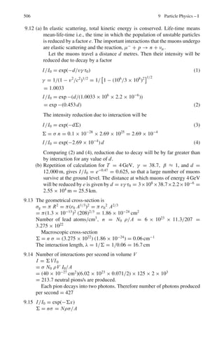
![7.3 Solutions 423
where c1 is another constant.
k log 3.36 + log(1622 × 365) = c1 (2)
k log 3.85 + log 138 = c1 (3)
Solving (2) and (3), k = 61.46 and c1 = 36.5. Using the values of k and c1
in (1) 61.46 log 6.97 + log T = 36.5
Solving for T , we find T = 4.79 × 10⁻¹⁶
days = 4.14 × 10⁻¹¹
s
7.105 For α-decay we use the equation
λ = 1/ τ = 1021
exp(−2 π zZ/137 β) (1)
T1/2(1)/T1/2(2) = τ1/τ2 = exp(2 π zZ1/137 β1)/ exp(2 π zZ2/137 β2) (2)
For 88Ra226
decay put Z1 = 86 for the daughter nucleus, z = 2 for α-particle
and β1 = (2E/Mc2
)1/2
= (2 × 4.9/3728)1/2
= 0.05127
For 90Th226
decay, put Z2 = 88 for daughter nucleus and z = 2 for α-particle
and β2 = (2 × 6.5/3728)1/2
= 0.05905
Using the values in (2), we find
τ1/τ2 = 5.19 × 10⁷
7.3.11 Beta-Decay
7.106 The selection rules for allowed transitions in β-decay are:
Δ I = 0
Ii = 0 → If = 0 allowed
Δ π = 0
⎫
⎬
⎭
Fermi Rule
Δ I = 0, ±1
Ii = 0 → Ii = 0 forbidden
Δ π = 0
⎫
⎬
⎭
G.T. Rule
where I is the nuclear spin and π is the parity. In view of the above selection
rules the first transition is Fermi transition, the second one Gamow–Teller
transition. The third one occurs between two mirror nuclei 17
F and 17
O in
which the proton number and neutron number are interchanged. The con-
figuration of nucleus is very much similar in such nuclei, consequently the
wave functions are nearly identical. This leads to a large value for the overlap
integral. The log ft value for such transitions is small being in the range of
3–3.7. These are characterized by
ΔI = 0,±1 and Δπ = 0. The given transition 17
F →17
O is an example of
superallowed transition.
7.107 If the number of 23
Mg nuclides is N0 at t = 0, then at time t the number
decayed will be
N = N0[1 − exp(−λ t)] (1)
At t = t1, N1 = N0[1 − exp(−λ t)] (2)
At t = t2, N2 = N0[1 − exp(−λ t)] (3)](https://image.slidesharecdn.com/1000-solved-problems-in-modern-physics-220626164600-18e7ea67/85/1000-solved-problems-in-modern-physics-pdf-524-320.jpg)
![424 7 Nuclear Physics – I
Dividing (3) by (2)
N2/N1 = [1 − exp(−λt2)]/[1 − exp(−λ t1)]
N2/N1 = 2.66 = [1 − exp(−6 λ)]/[1 − exp(−2λ)]
= (1 − x3
)/(1 − x) = 1 + x + x2
(4)
where x = exp(−2λ)
Solving the quadratic equation for x, we find x = 0.885 = exp(−2λ)
whence the mean life time τ = 1/λ = 15.93 s
7.108 According to Fermi’s theory of β-decay, for E0 mec2
, the decay constant
λ =
G2
|Mif|2
E5
0
60π3(c)6
(1)
So that with the value G/3
c3
= 1.166 × 10⁻⁵
GeV−2
, (1) becomes λ =
1.11E5
0 |Mif|2
104 S−1
= 1.11×(3.5)5
×6
104
= 0.3466 s−1
Therefore, T1/2 = 0.693/0.3466 = 2.0 s. The experimental value is 0.8 s.
7.109 The mean energy of electrons
E =
E max
0
E n(E)dE/
E max
0
n(E) dE
Given n(E)dE = c
√
E(Emax − E)2
dE
where c = constant
E =
c
E max
0 E
√
E(Emax − E)2
dE
c
E max
0
√
E(Emax − E)2 dE
=
Emax
3
If all the electrons emitted are absorbed then the kinetic energy of the
electrons is converted into heat.
Heat evolved/sec = (mean energy)(no. of electrons emitted/second)
= (0.156) × (3.7 × 107
)/3 MeV/s = 1.92 × 10⁶
MeV/s
7.110 Let the threshold energy be Eν. In that case the particles in the CMS will be
at rest. Now, in the neutron decay
n → p + e−
+ ν̄ + 0.79 MeV
Mn − (Mp + Me) = 0.79
as ν̄ has zero rest mass
Mn + Me = Mp + 2me + 0.79 = Mp + 1.81
(the masses of electron and positron are identical, each equal to 0.511 MeV)
We use the invariance of
(Σ E)2
− |ΣP|2
= (Σ E∗
)2
− zero
where (∗
) refers to the CMS and total momentum of particles in CMS is zero
(Ev + Mp)2
= (Mn + Me)2
= (Mp + 1.81)2
Or Eν = 1.81 MeV.](https://image.slidesharecdn.com/1000-solved-problems-in-modern-physics-220626164600-18e7ea67/85/1000-solved-problems-in-modern-physics-pdf-525-320.jpg)
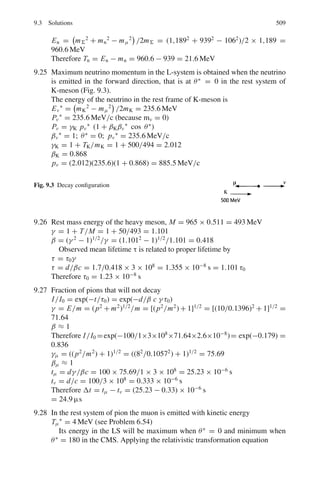
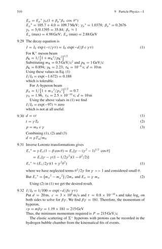
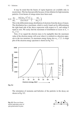
![428 8 Nuclear Physics – II
The shell model energy levels are:
*
1s1
2
+ *
1p3
2
, 1p1
2
+ *
1d5
2
, 2s1
2
, 1d3
2
+ *
1 f 7
2
+ *
2p3
2
, 1 f 5
2
, 2p1
2
, 1g9
2
+
*
1g7
2
, 2d5
2
, 2d3
2
, 3s1
2
, 1h 11
2
+
. . . (8.4)
Liquid drop model (8.5)
M(atom) = Z MH + (A − Z)Mn − Δ (8.6)
Δ = mass defect
P =
M − A
A
= packing fraction. (8.7)
1 amu =
1
12
of atomic mass of 12
C atom (8.8)
f =
B.E
A
(8.9)
1 amu = 931.5 Mev (8.10)
1 amu = 1.66 × 10⁻²⁷
kg (8.11)
The f-A curve is shown in Fig. 8.1. A more detailed diagram is shown in
Problem 8.40
Fig. 8.1 BE/A Versus A
Stability against decay
β−
− decay : M(Z, A) ≤ M(Z + 1, A) (8.12)
β+
− decay : M(Z + 1, A) ≤ M(Z, A) + 2Me (8.13)
e−
capture : M(Z + 1, A) ≤ M(Z, A) (8.14)
α − decay : M(Z, A) ≤ M(Z − 2, A − 4) + MHe4 (8.15)
Assuming that γ-ray precedes the decay, the energy released
Qβ− = [M(Z, A) − M(Z + 1, A)] c2
= Tmax + Tγ (8.16)
Qβ+ = [M(Z + 1, A) − M(Z, A)] c2
= 2Me c2
+ Tmax + Tγ (8.17)
QEC = [M(Z + 1, A) − M(Z, A)] c2
= Tv + Tγ (8.18)](https://image.slidesharecdn.com/1000-solved-problems-in-modern-physics-220626164600-18e7ea67/85/1000-solved-problems-in-modern-physics-pdf-529-320.jpg)
![432 8 Nuclear Physics – II
Fig. 8.4 Resonance and
potential sacttering and
absorption cross-sections as a
function of neutron energy
where g =
(2Ic + 1)
(2Ia + 1)(2Ix + 1)
(8.36)
Γaτa = ; Γbτb = (8.37)
σel =
π
k2
%
%Ares + Apot
%
%2
(8.38)
with Ares =
iΓn
(En − ER) + 1
2
iΓ
(8.39)
and Apot = exp(2ikR) − 1 (8.40)
Optical model
V = −U − iW (8.41)
U = vk1 (8.42)
W =
2
vk (8.43)
where v =
2E/m (8.44)
is the velocity of the incident nucleon.
k = (2mE)1/2
/; (8.45)
k1 = [2m(E + U)]1/2
/ (8.46)
K =
1
λ
=
A σ
vol
=
3σ
4πr3
0
(8.47)
Direct reactions (Reactions without compound nucleus formation)
1. Inelastic scattering
2. Charge exchange reactions
3. Nucleon transfer reactions](https://image.slidesharecdn.com/1000-solved-problems-in-modern-physics-220626164600-18e7ea67/85/1000-solved-problems-in-modern-physics-pdf-533-320.jpg)
![434 8 Nuclear Physics – II
If Ecm is the center of mass energy of the two interacting ions then the minimum
distance of approach is given by
rmin =
b
$
1 − V (rmin)
Ecm
(8.48)
8.2 Problems
8.2.1 Atomic Masses and Radii
8.1 Singly-charged lithium ions, liberated from a heated anode are accelerated by a
difference of 400 V between anode and cathode. They then pass through a hole
in the cathode into a uniform magnetic field perpendicular to their direction of
motion. The magnetic flux density is 8×10⁻²
Wb/m2
and the radii of the paths
of the ions are 8.83 and 9.54 cm, respectively. Calculate the mass numbers of
the lithium isotopes.
[Osmania University]
8.2 A narrow beam of singly charged 10
B and 11
B ions of energy 5 keV pass through
a slit of width 1 mm into a uniform magnetic field of 1,500 gauss and after a
deviation of 180◦
the ions are recorded on a photographic plate
(a) What is the spatial separation of the images.
(b) What is the mass resolution of the system?
[University of Manchester 1963]
8.3 Singly charged chlorine ions are accelerated through a fixed potential differ-
ence and then caused to travel in circular paths by means of a uniform field of
magnetic induction of 1,000 gauss. What increase in induction is necessary to
cause the mass 37 ion to follow the path previously taken by the mass 35 ion?
[University of London 1960]
8.4 27
14Si and 27
13Al are mirror nuclei. The former is a positron emitter with Emax =
3.48 MeV. Determine r0.
8.5 Use the uncertainty relation to estimate the kinetic energy of the nucleon, the
nuclear radius is about 5 × 10⁻¹³
cm and the mass of a proton is about 2 ×
10−24
g.
[University of Bristol 1969]
8.6 14
O is a positron emitter decaying to an excited state of 14
N. The 14
N
γ - rays have an energy of 2.313 MeV and the maximum energy of the positron
is 1.835 MeV. The mass of 14
N is 14.003074 amu and that of electron is
0.000548 amu. Find the mass of 14
O in amu.](https://image.slidesharecdn.com/1000-solved-problems-in-modern-physics-220626164600-18e7ea67/85/1000-solved-problems-in-modern-physics-pdf-535-320.jpg)
![8.2 Problems 435
8.2.2 Electric Potential and Energy
8.7 Derive an expression for the electrostatic energy of a spherical nucleus of radius
R assuming that the charge q = Ze is uniformly distributed homogeneously in
the nuclear volume.
8.8 A charge q is uniformly distributed in a sphere of radius R. Obtain an expres-
sion for the potential V (r) at a point distant r from the centre (r R).
8.2.3 Nuclear Spin and Magnetic Moment
8.9 Suppose a proton is assumed to be a classical particle rotating with angular
velocity of 2.6 × 10²³
rad/s about its axis. If it posseses a rotational energy of
537.5 MeV, then show that it has angular momentum equal to h.
8.10 (a) A D5/2 term in the optical spectrum of 39
19K has a hyperfine structure with
four components. Find the spin of the nucleus.
(b) In (a) what interval ratios in the hyperfine quadruplet are expected?
8.11 Given that the proton has a magnetic moment of 2.79 magnetons and a spin
quantum number of one half, what magnetic field strength would be required
to produce proton resonance at a frequency of 60 MHz in a nuclear magnetic
resonance spectrometer?
8.12 In a nuclear magnetic experiment for the nucleus 25Mn55
of dipole moment
3.46 μN , the magnetic field employed is 0.8 T. Find the resonance frequency.
You may assume J = 7/2, μN = 3.15 × 10⁻¹⁴
MeV T−1
8.2.4 Electric Quadrupole Moment
8.13 Show that for a homogeneous ellipsoid of semi axes a, b the quadrupole
moment is given by Q = 2
5
Ze(a2
− b2
)
8.14 Estimate the ratios of the major to minor axes of 181
73 Ta and 123
51 Sb. The
quadrupole moments are +6 × 10⁻²⁴
cm2
for Ta and −1.2 × 10⁻²⁴
cm2
for
Sb (Take R = 1.5 A1/3
fm)
[Saha Institute 1964]
8.15 Show that the electric quadrupole moment of a nucleus vanishes for
(a) Spherically symmetric charge distribution
(b) Nuclear spin I = 0 or I = 1/2
8.16 Show that for a rotational ellipsoid of small eccentricity and uniform charge
density the quadrupole moment is given by Q = 4
5
ZRΔR. Assuming that the
quadrupole moment of 181
71 Ta is 4.2 barns, estimate its size.](https://image.slidesharecdn.com/1000-solved-problems-in-modern-physics-220626164600-18e7ea67/85/1000-solved-problems-in-modern-physics-pdf-536-320.jpg)
![436 8 Nuclear Physics – II
8.2.5 Nuclear Stability
8.17 In general only the heavier nuclei tend to show alpha decay. For large A it is
found that B/A = 9.402 − 7.7 × 10⁻³
A.
Given that the binding energy of alpha particles is 28.3 MeV, show that
alpha decay is energetically possible for A 151.
[University of Wales, Aberystwyth, 2003]
8.18 For the nucleus 16
O the neutron and proton separation energies are 15.7 and
12.2 MeV, respectively. Estimate the radius of this nucleus assuming that the
particles are removed from its surface and that the difference in separation
energies is due to the Coulomb potential energy of the proton.
[University of Wales, Aberystwyth 2004]
8.19 By considering the general conditions of nucleus stability show that the
nucleus 229
90 Th will decay and decide whether the decay will take place by
α or β emission.
The atomic mass excesses of the relevant nuclei are:
Element 4
2He 225
88 Ra 229
89 Ac 229
90 Th 229
91 Pa
Mass excess amu ×10−6
2,603 23,528 32,800 31,652 32,022
8.20 The masses of 64
28Ni, 64
29Cu and 64
30Zn are as tabulated below. It follows that 64
29Cu
is radioactive. Detail the various possible decay modes to the ground state
of the daughter nucleus and give the maximum energy of each component,
ignoring the recoil energy. Compute the recoil energy in one of the cases and
verify that it was justifiable to ignore it.
Nuclide Atomic mass
64
28Ni 63.927959
64
29Cu 63.929759
64
30Zn 63.929145
[University of Bristol 1969]
8.21 28
13Al decays to 28
14Si via β−
emission with Tmax = 2.865 MeV. 28
14Si is in
the excited state which in turn decays to the ground state via γ -emission.
Find the γ -ray energy. Take the masses 28
Al = 27.981908 amu, 28
Si =
27.976929 amu.
8.22 22
11Na decays to 22
10Ne via β+
with Tmax = 0.542 MeV followed by γ -decay
with energy 1.277 MeV. If the mass of 22
Ne is 21.991385 amu, determine the
mass of 22
Na in amu.
8.23 7
4Be undergoes electron capture and decays to 7
3Li. Investigate if it can decay
by the competitive decay mode of β+
emission. Take masses 7
4Be = 7.016929
amu, 7
3Li = 7.016004 amu.](https://image.slidesharecdn.com/1000-solved-problems-in-modern-physics-220626164600-18e7ea67/85/1000-solved-problems-in-modern-physics-pdf-537-320.jpg)
![8.2 Problems 437
8.2.6 Fermi Gas Model
8.24 In the Fermi gas model the internal energy is given by U =
3
5
AEF, where
A is the mass number and EF is the Fermi energy. For a nucleus of volume
V with N = Z = A/2. A = KVEF
3/2
where K is a constant. Using the
thermodynamic relation, p = −
∂U
∂V
s
, show that the pressure is given by
p =
2
5
ρn EF, where ρn is the nucleon density.
8.25 Assuming that in a nucleus N = Z = A/2, calculate the Fermi momentum,
Fermi energy EF, and the well depth.
8.2.7 Shell Model
8.26 A certain odd-parity shell model state can accommodate up to a maximum of
12 nucleons. What are its j and l values?
8.27 The shell model energy levels are in the following way
[1s1/2][1p3/2, 1p1/2][1d5/2, 2s1/2, 1d3/2][1 f7/2][2p3/2, 1 f5/2, 2p1/2, 1g9/2]
[1g7/2, 2d5/2, 2d3/2, 3s1/2, 1h11/2] . . .
Assuming that the shells are filled in the order written, what spins and pari-
ties should be expected for the ground state of the following nuclei?
7
3Li, 16
8 O, 17
8 O, 39
19K, 45
21Sc.
8.28 Find the gap between the 1p1/2 and 1d5/2 neutron shells for nuclei with mass
number A ≈ 16 from the total binding energy of the 15
O (111.9556 MeV),
16
O (127.6193 MeV) and 17
O (131.7627 MeV) atoms.
8.29 Compute the expected shell-model quadruple moment of 209
Bi(9/2
−
)
8.30 From the shell model predictions find the ground state spin and parity of the
following nuclides:
3
2He; 20
10Ne; 27
13Al; 41
21Sc;
8.31 Making use of the shell model, write down the ground state configuration of
protons and neutrons for 12
6 C and the next three isotopes of increasing A. Give
the spin and parity assignment for the ground state of 13
6 C and compare this
with the equivalent assignments for the ground state of 15
6 C.
8.32 How does the shell model predict
7−
2
for the ground state spin parity of 41
20Ca.
What does the model predict about the spin and parities of the ground states
of 30
14Si and 14
7 N?
[University of Cambridge, Tripos 2004]](https://image.slidesharecdn.com/1000-solved-problems-in-modern-physics-220626164600-18e7ea67/85/1000-solved-problems-in-modern-physics-pdf-538-320.jpg)
![438 8 Nuclear Physics – II
8.2.8 Liquid Drop Model
8.33 Deduce that with ac = 0.72 MeV and as = 23 MeV the ratio zmin/A is approx-
imately 0.5 for light nuclei and 0.4 for heavy nuclei.
[Royal Holloway, University of London 1998]
8.34 Determine the most stable isobar with mass number A = 64.
8.35 The masses (amu) of the mirror nuclei 27
13Al and 27
14Si are 26.981539 and
26.986704 respectively. Determine the Coulomb’s coefficient in the semi
emperical mass formula.
8.36 If the binding energies of the mirror nuclei 41
21Sc and 41
20Ca are 343.143 V and
350.420 MeV respectively, estimate the radii of the two nuclei by using the
semi empirical mass formula [e2
/4πε0 = 1.44 MeV fm]
8.37 The empirical mass formula (neglecting a term representing the odd – even
effect) is M(A, Z) = Z(mp + me) + (A − Z)mn − αA + β A2/3
+ γ (A −
2Z)2
/A + εZ2
A−1/3
where α, β, γ and ε are constants. By finding the min-
imum in M(A, Z) for constant A obtain the expression Zmin = 0.5A(1 +
0.25A2/3
ε/γ )−1
for the value of Z which corresponds to the most stable
nucleus for a set of isobars of mass number A.
[Royal Holloway, University of London 1998]
8.38 The binding energy of a nucleus with atomic number Z and mass number A
can be expressed by Weisacker’s semi – empirical formula
B = av A − as A2/3
−
ac Z2
A1/3
− aa
(N − Z)2
A
−
ap
A1/2
where av = 15.56 MeV, as = 17.23 MeV,
ac = 0.697 MeV, aa = 23.285 MeV, ap = −12, 0, 12 MeV
for even-even, odd-even (or even-odd) or odd-odd nucleus respectively.
Estimate the energy needed to remove one neutron from nucleus 40
20Ca.
8.39 (a) Consider the alpha particle decay 230
90 Th →226
88 Ra + α and use the follow-
ing expression to calculate the values of the binding energy B for the two
heavy nuclei involved in this process.
B = av A − as A2/3
− ac
Z(Z − 1)
A1/3
− aa
(N − Z)2
A
− ap A−3/4
where values for the constants av, as, ac, aa and ap are respectively 15.5,
16.8, 0.72, 23.0 and −34.5 MeV. Given that the total binding energy of the
alpha particle is 28.3 MeV, find the energy Q released in the decay.
(b) This energy appears as the kinetic energy of the products of the decay.
If the original thorium nucleus was at rest, use conservation of momen-
tum and conservation of energy to find the kinetic energy of the daughter
nucleus 226
Ra.](https://image.slidesharecdn.com/1000-solved-problems-in-modern-physics-220626164600-18e7ea67/85/1000-solved-problems-in-modern-physics-pdf-539-320.jpg)
![8.2 Problems 439
8.40 The following plot (Fig. 8.7) shows the average binding energy per nucleon
for stable nuclei as a function of mass number.
Explain how the mass of a nucleus can be calculated from this plot and esti-
mate the mass of 235
92 U.
Briefly describe the main features of the plot in the context of nuclear
models such as the liquid Drop Model, the Fermi Gas Model and the Nuclear
Shell Model.
In terms of the Liquid Drop Model, explain why nuclear fission and fusion
are possible and estimate the energy released when a nucleus of 235
92 U under-
goes fission into the fragments 87
35Br and 145
57 La with the release of three prompt
neutrons.
[University of Cambridge, Tripos 2004]
Fig. 8.7 B/A versus A plot
8.41 Investigate using liquid drop model, the β stability of the isobars 127
53 I and
127
54 Xe given that
127
51 Sb → β−
+127
52 Te + 1.60 MeV
127
55 Cr → β+
+127
54 Xe + 1.06 MeV
[University of London 1969]
8.42 The empirical mass formula is
A
Z M = 0.99198 A − 0.000841 Z + 0.01968 A2/3
+ 0.0007668 Z2
A−1/3
+0.09966(Z − A/2)2
A−1
− δ
in atomic mass units, where δ = ±0.01204 A−1/2
or 0.
Determine whether or not the nuclide 27
12Mg is stable to β decay.
[University of Newcastle 1966]
8.2.9 Optical Model
8.43 Show that the imaginary part of the complex potential V = −(U + iW) in the
optical model has the effect of removing particle flux from the elastic channel.](https://image.slidesharecdn.com/1000-solved-problems-in-modern-physics-220626164600-18e7ea67/85/1000-solved-problems-in-modern-physics-pdf-540-320.jpg)
![440 8 Nuclear Physics – II
8.44 For neutrons with kinetic energy 100 MeV incident on nuclei with mass num-
ber A = 120, the real and imaginary parts of the complex potential are approx-
imately −25 and −10 MeV, respectively. On the basis of these data, estimate
(i) the deBroglie wavelength of the neutron inside the nucleus
(ii) the probability that the neutron is absorbed in passing through the nucleus
8.2.10 Nuclear Reactions (General)
8.45 13
N is a positron emitter with an end point energy of 1.2 MeV. Determine the
threshold of the reaction p +13
C →13
N + n, if the neutron – hydrogen atom
mass difference is 0.78 MeV.
[Osmania University 1964]
8.46 The reaction, p +7
3 Li →7
4 Be + n, is known to be endothermic by 1.62 MeV.
Find the total energy released when 7
Be decays by K capture and calculate the
energy carried off by the neutrino and recoil nucleus, respectively.
(Mpc2
= 938.23 MeV, Mnc2
= 939.52 MeV, Mec2
= 0.51 MeV)
[University of Bristol 1960]
8.47 If a target nucleus has mass number 24 and a level at 1.37 MeV excita-
tion, what is the minimum proton energy required to observe scattering from
this level.
[Osmania University 1966]
8.48 The nuclear reaction which results from the incidence of sufficiently energetic
α-particles on nitrogen nuclei is 4
2He +14
7 N → X +1
1 H. What is the decay
product X? What is the minimum α-particle kinetic energy (in the laboratory
frame) required to initiate the above reaction?
(Atomic masses in amu: 1
H = 1.0081; 4
He = 4.0039; 14
N = 14.0075; X =
17.0045)
[University of Manchester]
8.49 The Q values for the reactions 2
H(d, n) 3
He and 2
H(d, p) 3
H are 3.27 MeV and
4.03 MeV, respectively. Show that the difference between the binding energy
of the 3
H nucleus and that of the 3
He nucleus is 0.76 MeV and verify that this
is approximately the magnitude of Coulomb energy due to the two protons of
the 3
He nucleus. (Distance between the protons in the nucleus 31/3
× 1.3 fm).
[University of London 1968]
8.50 Thermal neutrons are captured by 10
5 B to form 11
5 B which decays by α-particle
emission to Li. Write down the reaction equation and calculate
(a) The Q-Value of the decay in MeV
(b) The Kinetic energy of the α-particles in MeV.
(Atomic masses: 10
5 B = 10.01611 amu; 1
0n = 1.008987 amu; 7
3Li
= 7.01822 amu; 4
2He = 4.003879 amu; 1 amu = 931 MeV)
[University of Bristol 1967]](https://image.slidesharecdn.com/1000-solved-problems-in-modern-physics-220626164600-18e7ea67/85/1000-solved-problems-in-modern-physics-pdf-541-320.jpg)
![8.2 Problems 441
8.51 Consider the reaction 27
Al(p, n)27
Si. The positrons from the decay of 27
Si are
observed and their spectrum is found to have an end – point energy of 3.5 MeV.
Derive the Q value of the (p, n) reaction, and find the threshold proton energy
for the reaction given that the neutron – proton mass difference is 0.8 MeV.
[University of Manchester 1963]
8.52 The Q value of the 3
H(p, n)3
He reaction is −0.764 MeV. Calculate (a) the
threshold energy for appearance of neutrons in the forward direction (b) the
threshold for the appearance of neutron in the 90◦
direction.
[University of Liverpool 1960]
8.53 When 30
Si is bombarded with a deuteron, 31
Si is formed in its ground state
with the emission of a proton. Determine the energy released in this reaction
from the following information:-
31
Si →31
p + β−
+ 1.51 MeV
30
Si + d → 31
p + n + 5.10 MeV
n → p + β−
+ ν + 0.78 MeV
[University of London 1960]
8.54 The nucleus 12
C has an excited state at 4.43 MeV. You wish to investigate
whether this state can be produced in inelastic scattering of protons through
90◦
by a carbon target. If you have access to a beam of protons of kinetic
energy 15 MeV, what is the kinetic energy of the scattered protons for which
you must look?
[University of Bristol 1966]
8.55 A thin hydrogenous target is bombarded with 5 MeV neutrons, and a detec-
tor is arranged to collect those protons emitted in the same direction as the
neutron beam. The neutron beam is replaced by a beam of γ -rays; calculate
the photon energy needed to produce protons of the same energy as with the
neutron beam.
[Osmania University]
8.56 Protons of energy 5 MeV scattering from 10
5 B at an angle of 45◦
show a peak
in the energy spectrum of the scattered protons at an energy of 3.0 MeV
(a) To what excitation energy of 10
5 B does this correspond?
(b) What is the expected energy of the scattered protons if the scattering is
elastic?
8.57 Calculate the energy of protons detected at 90◦
when 2.1 MeV deutrons are
incident on 27
Al to produce 28
Al with an energy difference Q = 5.5 MeV.
[Royal Holloway University of London 1998]
8.58 The reaction 2
H +1
H →3
He + γ + 5.3 MeV occurs with the deuterons and
proton at rest. Estimate the energy of the helium nucleus.
If the reaction occurs in a region of the sun where the temperature is about
1.7 × 10⁷
K, estimate how close the deuteron and proton must approach for
fusion to occur.
[Osmania University]](https://image.slidesharecdn.com/1000-solved-problems-in-modern-physics-220626164600-18e7ea67/85/1000-solved-problems-in-modern-physics-pdf-542-320.jpg)
![442 8 Nuclear Physics – II
8.59 The Q- value of the reaction 16
O(d, n)17
F is −1.631 MeV, while that of the
reaction 16
O(d, p)17
O is +1.918 MeV. Which is the unstable member of the
pair 17
O−17
F, and what is the maximum energy of β-particles it emits? (n−1
H
mass difference is 0.782 MeV)
[University of Manchester 1958]
8.60 An aluminum target is bombarded by α-particles of energy 7.68 MeV, and the
resultant proton groups at 90◦
were found to possess energies 8.63, 6.41, 5.15
and 3.98 meV. Draw an energy level diagram of the residual nucleus, using the
above information.
[Osmania University 1963]
8.61 If the Q-value for the 3
H(p, n)3
He reaction is −0.7637 MeV and tritium (3
H)
emits negative β-particles of end point energy 18.5 KeV, calculate the differ-
ence in mass between the neutron and the hydrogen atom.
[Andhra University]
8.62 The reaction 3
H(d, n)4
He has Q value of 17.6 MeV. What is the range of neu-
tron energies that may be obtained from this reaction for an incident deuteron
beam of 300 KeV?
[Osmania University 1970]
8.63 A target of 181
Ta is bombarded with 5 MeV protons to form 182
W in an excited
state. Calculate the energy of the excited state (ignore the coulomb barrier and
assume the target nuclei at rest). If 182
W in the same excited state were pro-
duced by bombarding a hydrogen target with energetic Ta nuclei, what energy
would be needed? The atomic masses in amu are: 1
H1 = 1.007825; 181
73 Ta =
180.948007; 182
74 W = 181.948301
[University of Durham 1963]
8.64 In the reaction 48
Ca +16
O →49
Sc +15
N, the Q-value is −7.83 MeV. What is
the minimum kinetic energy of bombarding 16
O ions to initiate the reaction?
At this energy, estimate the orbital angular momentum in units of of the ions
for grazing collision. Take R = 1.1 A1/3
fm.
8.2.11 Cross-sections
8.65 Calculate the thickness of Indium foil which will absorb 1% of neutrons inci-
dent at the resonance energy for Indium (1.44 eV) where σ = 28, 000 barns.
At. Wt of Indium = 114.7 amu, density of Indium = 7.3 g/cm3
.
[Andhra University]
8.66 60
Co is produced from natural cobalt in a reactor with a thermal neutron flux
density of 5 × 10¹²
n cm−2
s−1
. Determine the maximum specific activity.
Given σact = 20 b.](https://image.slidesharecdn.com/1000-solved-problems-in-modern-physics-220626164600-18e7ea67/85/1000-solved-problems-in-modern-physics-pdf-543-320.jpg)
![8.2 Problems 443
8.67 Natural Cobalt is irradiated in a reactor with a thermal neutron flux density of
3 × 10¹²
n cm−2
s−1
. How long an irradiation will be required to reach 20%
of the maximum activity? Given T1/2 = 5.3 years
8.68 In a scattering experiment an aluminum foil of thickness 10 μm is placed in
a beam of intensity 8 × 10¹²
particles per second. The differential scattering
cross-section is known to be of the form
dσ
dΩ
= A + B cos2
θ
where A, B are constants, θ is scattering angle and Ω is the solid angle.
With a detector of area 0.01 m2
placed at a distance of 6 m from the foil, it is
found that the mean counting rate is 50 s−1
when θ is 30◦
and 40 s−1
when θ
is 60◦
. Find the values of A and B. The mass number of aluminum is 27 and
its density is 2.7 g/cm2
.
8.69 A thin target of 48
Ca with 1.3×10¹⁹
nuclei per cm2
is bombarded with a 10 nA
beam of α particles. A detector, subtending a solid angle of 2×10⁻³
steradians,
records 15 protons per second. If the angular distribution is measured to be
isotropic, determine the total cross section for the 48
Ca(α, p) reaction.
[University of Cambridge, Tripos 2004]
8.2.12 Nuclear Reactions via Compound Nucleus
8.70 Cadmium has a resonance for neutrons of energy 0.178 eV and the peak value
of the total cross-section is about 7,000 b. Estimate the contribution of scatter-
ing to this resonance.
[Osmania University 1964]
8.71 A nucleus has a neutron resonance at 65 eV and no other resonances nearby.
For this resonance, Γn = 4.2 eV, Γγ = 1.3 eV and Γα = 2.7 eV, and all
other partial widths are negligible. Find the cross-section for (n, γ ) and (n, α)
reactions at 70 eV.
[Osmania University]
8.72 Neutrons incident on a heavy nucleus with spin JN = 0 show a resonance at an
incident energy ER = 250 eV in the total cross-section with a peak magnitude
of 1,300 barns, the observed width of the peak being Γ = 20 eV. Find the
elastic partial width of the resonance.
[University of Bristol 1970]
8.2.13 Direct Reactions
8.73 The reaction d +14
N → α +12
C has been used to test the principle of detailed
balance which relates the cross-section σab for a reaction a + x → b + y, to
the cross-section for the inverse reaction and has the form
(2Sa + 1) (2Sx + 1) Pa
2
σab = (2Sb + 1) (2Sy + 1) Pb
2
σba](https://image.slidesharecdn.com/1000-solved-problems-in-modern-physics-220626164600-18e7ea67/85/1000-solved-problems-in-modern-physics-pdf-544-320.jpg)
![444 8 Nuclear Physics – II
The reaction above will take place for low energy incident deuterons in a
s-wave state leaving the 12
C nucleus in the ground state.
Given that the deuteron has spin 1 and positive parity while the alpha par-
ticle has zero spin and positive parity, estimate the spin of 14
N in the ground
state.
Can the alpha particle come off with orbital angular momentum l = 1?
If the incident kinetic energy of the deuteron is 20 MeV in the laboratory
frame, calculate the laboratory kinetic energy at which α’s should scatter from
12
C to test the principle of detailed balance. What is the expected ratio between
the cross-sections for the direct and inverse reactions? Atomic masses of
14
N, 2
H and 4
He are 14.003074, 2.014102, 4.002603 amu respectively. 1 amu
= 931.44 MeV.
[University of Bristol 1969]
8.74 A beam of 460 MeV deuterons impinges on a target of bismuth. Given the
binding energy of the deuteron is 2.2 MeV, compute the mean energy, spread
in energy and the angle of the cone in which the neutrons are emitted.
[Osmania University 1975]
8.2.14 Fission and Nuclear Reactors
8.75 1.0 g of 23
Na of density 0.97 is placed in a reactor at a region where the ther-
mal flux is 1011
/cm2
/s. Set up the equation for the production of 24
Na and
determine the saturation activity that can be produced. The half-life of 24
Na is
15 h, and the activation cross-section of 23
Na is 536 millibarns.
[Osmania University 1964]
8.76 Suppose 100 mg of gold (197
79 Au) foil are exposed to a thermal neutron flux
of 1012
neutrons/cm2
/s in a reactor. Calculate the activity and the number
of atoms of 198
Au in the sample at equilibrium [Thermal neutron activation
cross-section for 197
Au is 98 barns and half-life for 197
Au is 2.7 h]
[Osmania University]
8.77 Estimate the energy released in fission of 238
92 U nucleus, given ac = 0.59 MeV
and as = 14.0 MeV.
[Osmania University 1962]
8.78 A small container of Ra–Be is embedded in the middle of a sphere of paraffin
wax of a few cm radius so as to form a source of (predominantly) thermal
neutrons. This source is placed at the centre of a very large block of graphite.
Derive an expression for the density of thermal neutrons at a large distance r
from the source in terms of the source strength Q, the diffusion coefficient D
and diffusion length L.
A small BF3 counter is placed in the graphite at a distance of 3 m from
the above source contains 1020
atoms of 10
B. The cross-section of 10
B for
the thermal neutron capture follows a 1/v law and has a magnitude of 3,000](https://image.slidesharecdn.com/1000-solved-problems-in-modern-physics-220626164600-18e7ea67/85/1000-solved-problems-in-modern-physics-pdf-545-320.jpg)
![8.2 Problems 445
barns for a neutron velocity v = 2, 200 m/s. If the counting rate is 250/min,
calculate the value of Q. Given L = 50 cm; D = 5 × 10⁵
cm2
/s.
[University of Bristol 1959]
8.79 Calculate the thermal utilization factor for a heterogeneous lattice made up of
cylindrical uranium rods of diameter 3 cm and pitch 18 cm in graphite
Take the flux ratio φm/φU as 1.6
Densities : Uranium = 18.7 × 10³
kg m−3
, Graphite = 1.62 × 10³
kg m−3
Absorption cross-sections σav = 7.68 b; σam = 4.5 × 10⁻³
b.
[University of Durham 1961]
8.80 Calculate approximately, using one-group theory results, the critical size of a
bare spherical reactor, given k∞ = 1.54 and Migration area M2
= 250 cm2
.
8.81 Assuming the energy released per fission of 235
U is 200 MeV, calculate the
amount of 235
U consumed per day in Canada India reactor “Cirus” operating
at 40 MW of power.
8.82 Assuming that the energy released per fission of 235
92 U is 200 MeV, calculate the
number of fission processes that should occur per second in a nuclear reactor
to operate at a power level of 20,000 kW. What is the corresponding rate of
consumption of 235
92 U.
[University of London 1959]
8.83 (a) Assume that in each fission of 235
U, 200 MeV is released. Assuming that
5% of the energy is wasted in neutrinos, calculate the amount of 235
U
burned which would be necessary to supply at 30% efficiency, the whole
annual electricity consumption in Britain 50 × 109
kWh
(b) A thermal reactor contains 100 tons of natural uranium (density 19) and
operates at a power of 100 MW (heat). Assuming that the thermal cross-
section of 235
U is 550 barns and that the uranium contains 0.7 % of 235
U.
Calculate the neutron flux near the centre of the reactor by neglecting neu-
tron losses from the outside, and assuming flux constant through out the
lattice.
[University of Liverpool 1959]
8.84 If the elastic scattering of neutrons by hydrogen nuclei is isotropic in the centre
of mass system, show that
ln(E1/E2) = 1
where E1 and E2 are respectively the kinetic energies of a neutron before and
after the collision.
[University of London 1969]
8.85 (a) Estimate the average number of collisions required to reduce fast fission
neutrons of initial energy 2 MeV to thermal energy (0.025 eV) in graphite
moderator.
(b) Calculate the corresponding slowing-down time given that Σs=0.385 cm−1](https://image.slidesharecdn.com/1000-solved-problems-in-modern-physics-220626164600-18e7ea67/85/1000-solved-problems-in-modern-physics-pdf-546-320.jpg)
![446 8 Nuclear Physics – II
8.86 Show that a homogeneous, natural uranium-graphite moderated assembly can
not become critical. Use the following data:
400 moles of graphite per mole of uranium
Natural uranium Graphite
σa(U) = 7.68 b σa(M) = 0.0032 b
σs (U) = 8.3 b σs(M) = 4.8 b
ε = 1.0; η = 1.34 ξ = 0.158
[Osmania University 1964]
8.87 A point source of thermal neutrons is placed at the centre of a large sphere of
beryllium.
Deduce the spatial distribution of neutron density in the sphere. Estimate
what its radius must be if less than 1% of the neutrons are to escape through
the surface. Find also the neutron density near the surface in this case in terms
of the source strength.
At. Wt of beryllium = 9
Density of beryllium = 1.85 g/cc
Avagadro number = 6 × 10²³
atoms/g atom
Thermal neutron scattering cross-section on beryllium = 5.6 barns
Thermal neutron capture cross-section on beryllium = 10 mb (at velocity
v = 2,200 m/s)
[University of Bristol 1961]
8.88 Calculate the steady state neutron flux distribution about a plane source emit-
ting Q neutrons/s/cm2
in an infinite homogeneous diffusion medium. Assume
that neutrons are not produced in any region of interest.
8.89 Calculate the thermal diffusion time for graphite. Use the data:
σa(C) = 0.003 b, ρc = 1.62 g cm−3
. Average thermal neutron speed
= 2,200 m/s.
8.90 Estimate the generation time for neutrons in a critical reactor employing 235
U
and graphite. Use the following data:
Σ
a
= 0.0006 cm−1
; B2
= 0.0003; L2
= 870 cm2
; v = 2200 ms.
8.91 The spatial distribution of thermal neutrons from a plane neutron source kept
at a face of a semi-infinite medium of graphite was determined and found to
fit e−0.03x
law where x is the distance along the normal to the plane of the
source. If the only impurity in the graphite is boron, calculate the number of
atoms of boron per cm3
in the graphite if the mean free path for scattering
and absorption in graphite are 2.7 and 2,700 cm, respectively. The absorption
cross-section of boron is 755 barns.
[Osmania University 1964]](https://image.slidesharecdn.com/1000-solved-problems-in-modern-physics-220626164600-18e7ea67/85/1000-solved-problems-in-modern-physics-pdf-547-320.jpg)
![8.3 Solutions 447
8.92 Assuming that the elastic scattering of low energy neutrons is isotropic,
show that the mean energy of the neutron after each collision will be
Ef = (A2
+ 1)Ei/(A + 1)2
where A is the mass number of the target nucleus. Determine the number of
collisions needed to thermalize fission neutrons (2 MeV) in graphite (A = 12).
8.2.15 Fusion
8.93 Determine the range of neutrino energies in the solar fusion reaction, p+ p →
d + e+
+ ν. Assume the initial protons have negligible kinetic energy and that
the binding energy of the deuteron is 2.22 MeV, mp = 938.3 MeV/c2
and
md = 1875.7 MeV/c2
and me = 0.51 MeV/c2
.
8.94 If the kinetic energy of the deuterons in the fusion reaction D + D →3
2He +
n + 3.2 MeV can be neglected, what is the kinetic energy of the neutron?
8.95 (a) It is estimated that the deutrons have to come within 100 fm of each other
for fusion to proceed. Calculate the energy that the deuterons must possess
to overcome the electrostatic repulsion.
(b) If the energy is supplied by the thermal energy of the deutrons, what is the
temperature of the deuteron?
[e2
/4πε0 = 1.44 MeV fm, Boltzmann constant k = 1.38 × 10⁻²³
J K−1
]
(c) In (b) the actual required temperature is lower than the estimated value.
Explain the mechanism by which the fusion reaction may proceed.
8.96 In a fusion reactor, the D-T reaction with Q value of 17.62 MeV is employed.
Assuming that the deuteron density is 7×10¹⁸
m−3
and the experimental value
σDT · v = 10−22
m3
s
−1
and that equal number of deuterons and tritons
exist in the plasma at energy 10 keV, calculate the confinement time if the
Lawson criterion is just satisfied.
8.3 Solutions
8.3.1 Atomic Masses and Radii
8.1 An ion of charge q will pick up kinetic energy, T = qV in dropping through a
P.D of V volts. In a magnetic induction B perpendicular to its path, the ion of
momentum p will describe a circular path of radius r given by
p = qBr =
√
2MT =
2MqV
M =
q B2
r2
2V
(1)
For the first ion, q = 1.6 × 10⁻¹⁹
C, B = 0.08, r = 0.0883 m and V =
400 V. Substituting these values in (1) we get
M1 = 9.98 × 10⁻²⁷
kg](https://image.slidesharecdn.com/1000-solved-problems-in-modern-physics-220626164600-18e7ea67/85/1000-solved-problems-in-modern-physics-pdf-548-320.jpg)
![8.3 Solutions 449
ΔEc =
3
5
.
1
4πε0
.
e2
R
[Z(Z + 1) − Z(Z − 1)]
=
6Ze2
5R
.
e2
4πε0
= 1.2 × 1.44
Z
R
MeV-fm
Equating ΔEc to MSi − MA = 3.48 + 2 × 0.51 = 4.5 MeV, and Z = 13,
we find R from which ro = R/A1/3
can be determined, where A = 27. Thus
ro = 1.66 fm.
8.5 ΔPx .Δx = (uncertainty principle)
or cΔPx =
c
Δx
=
197.3 MeV − fm
5 fm
= 39.6 MeV
The kinetic energy T =
c2
p2
2Mc2
=
(39.6)2
2 × 940
= 0.83 MeV
8.6 The mass-energy equation for positron decay is
M(14
O) − M(14
N) = 2me +
Eβ (max) + Eγ
931.5
= 2 × 0.000548 +
1.835 + 2.313
931.5
= 0.005549
or M(14
O) = 14.003074 + 0.005549 = 14.008623 amu
8.3.2 Electric Potential and Energy
8.7 The charge density ρ = 3ze/4π R3
. Consider a spherical shell of radii r and
r + dr.
The volume of the shell is 4π r2
dr. The charge in the shell q
= (4πr2
dr)ρ.
The electrostatic energy due to the charge q
and the charge (q
) of the sphere
of radius r, which is 4
3
πr3
ρ, is calculated by imagining q
to be deposited at
the centre. The charge outside the sphere of radius r does not contribute to this
energy (Fig. 8.8). Thus
dU =
q
q
4πε0r
=
(4πr2
drρ)(4πr3
ρ/3)
4πε0r
=
4π
ε0
ρ2
r4
dr
The total electrostatic energy is obtained by integrating the above expression
in the limits 0 to R,
Fig. 8.8 Spherical shell of
radius R](https://image.slidesharecdn.com/1000-solved-problems-in-modern-physics-220626164600-18e7ea67/85/1000-solved-problems-in-modern-physics-pdf-550-320.jpg)

![454 8 Nuclear Physics – II
Therefore (a2
− b2
) = 14.79 fm2
(1)
Now, A =
4
3
πab2
ρ (2)
The nuclear charge density, ρ = 0.17 fm−3
(3)
Using the value of ρ and A = 181 in (2), we get
ab2
= 254.3 fm3
(4)
Solving (2) and (4) we find a = 7.1 fm, b = 6.0 fm
8.3.5 Nuclear Stability
8.17 Given B/A = 9.402 − 7.7 × 10⁻³
A
For the parent nucleus
B(A, Z) = 9.402A − 7.7 × 10⁻³
A2
For the product nucleus
B(A − 4, Z − 2) = 9.402(A − 4) − 7.7 × 10⁻³
(A − 4)2
B(∝) = 28.3
Condition that alpha decay is just energetically possible is
B(A, Z) = B(A − 4, Z − 2) + B(∝)
Or 9.402A − 7.7 × 10⁻³
A2
= 9.402(A − 4) − 7.7 × 10⁻³
(A − 4)2
+ 28.3
Simplifying and solving for A, we find that A = 153. Thus, alpha decay is
energetically possible for A 153.
8.18 Sn − Sp = 15.7 − 12.2 = 3.5 =
3
5
×
e2
4πε0 R
[Z2
− (Z − 1)2
]
Substitute e2
/4πεo = 1.44 MeV fm and Z = 8 to find R = 3.7 fm.
8.19 An atom of mass M1 will decay into the product of mass M2 and α particle of
mass mα if M1 M2 + mα. Now the mass excess Δ = M − A.
For 229
Th, M1 = 229 + 0.031652 = 229.031652 amu. For α decay, the prod-
uct atom would be 225
Ra, and M2 = 225 + 0.023528 = 225.023528.
For α - particle, mα = 4 + 0.002603 = 4.002603
M2 + mα = 229.026131
Since, M1 M2 + mα, 229
Th will decay via α emission.
For β−
decay, M2 = 229 + 0.032022 = 229.032022
As M1 M2, decay via β−
emission is not possible. By the same argument
the decay of 229
Th to 229
Ac is not possible via β+
emission as M1 M2+2me.](https://image.slidesharecdn.com/1000-solved-problems-in-modern-physics-220626164600-18e7ea67/85/1000-solved-problems-in-modern-physics-pdf-555-320.jpg)
![8.3 Solutions 457
8.3.7 Shell Model
8.26 A state with quantum number j can accommodate a maximum number of
Nj = 2(2 j + 1) nucleons. Now j = l ± 1
2
and for Nj = 12, j = 5/2 and
l = 3 or 2. However, because the parity is odd and P = (−1)l
, it follows
that l = 3.
8.27 In the shell model the nuclear spin is predicted as due to excess or deficit of
a particle (proton or neutron) when the shell is filled. Its parity is determined
by the l value of the angular momentum, and is given by (−1)l
. For s- state,
l = 0, p – state, l = 1, d-state l = 2, f-state l = 3 etc.
For the ground state of the nuclei:
7
3Li: Spin is due to the third proton in P3/2 state.
Therefore Jπ
= (3/2)−
(∵ l = 1)
16
8 O: This is a doubly magic nucleus, and Jπ
= 0+
17
8 O: Spin is due to the 9th neutron in d5/2 state.
Therefore Jπ
= (5/2)+
(∵ l = 2)
39
19K: Spin is due to the proton hole in the d3/2 state.
Therefore Jπ
= (3/2)+
(∵ l = 2)
45
21Sc: spin is due to the 21st proton in the f7/2 state.
Therefore Jπ
= (7/2)−
(∵ l = 3)
8.28 The 15
O nucleus in the 1p1/2 shell is an 16
O nucleus deficit in one neutron,
its energy being B(15)–B(16), while 17
O in the 1 f5/2 shell is an 16
O nucleus
with a surplus neutron, its energy being B(16)–B(17). Thus the gap between
the shells is
E(1 f5/2) − E(1 p1/2) = B(16) − B(17) − [B(15) − B(16)]
= 2 B(16) − B(17) − B(15)
= 2 × 127.6193 − 131.7627 − 111.9556
= 11.52 MeV
8.29 Q = −
2 j − 1
2 j + 2
r2
For 209
Bi, j = 9/2, r2
= 3
5
R2
= 3
5
r2
0 A2/3
= 3
5
(1.2)2
(209)2/3
= 30.42 fm2
= 0.3 b
Q = −0.22 b
8.30 The spin and parity are determined as in Problem 8.27. The ground state spin
and parity for the following nuclides are:](https://image.slidesharecdn.com/1000-solved-problems-in-modern-physics-220626164600-18e7ea67/85/1000-solved-problems-in-modern-physics-pdf-558-320.jpg)
![458 8 Nuclear Physics – II
3
2He : Jπ
= (1/2)+
The state due to neutron hole is 1s1/2
20
10Ne : Jπ
= (0)+
The protons and neutrons complete the sub-shell.
27
13Al : Jπ
= (5/2)+
The state of an extra neutron is 1d5/2
41
21Sc : Jπ
= (7/2)−
The state of an extra proton is 1 f7/2
8.31 For the nuclei 12
6 C, 13
6 C, 14
6 C and 15
6 C the ground state configuration of protons
is
1s1/2, 1p3/2
For neutrons it is
(1s1/2, 1p3/2), (1s1/21p3/2, 1p1/2), (1s1/2, 1p3/2, 1p1/2) and
(1s1/2, 1p3/2, 1p1/2, 1D5/2) respectively
The spin and parity assignment for 13
6 C is (1/2)−
and that for 15
6 C, it is
(1/2)+
.
8.32 Twenty neutrons and twenty protons fill up the third shell. The extra neutron
goes into the 1 f7/2 state. The spin and parity are determined by this extra
neutron. Therefore the spin is 7/2. The parity is determined by the l - value
which is 3 for the f-state. Hence the parity is (−1)l
= (−1)3
= −1.
The model predicts Jπ
= (0)+
for 30
14Si and Jπ
= (1)+
for 14
7 N nuclides.
8.3.8 Liquid Drop Model
8.33 Using the mass formula one can deduce the atomic number of the most stable
isobar. It is given by
Zmin =
A
2 + (ac/2as)A2/3
Zmin
A
=
1
2 + 0.0156A2/3
For light nuclei, say A = 10, the second term in the denominators is small,
and zmin/A = 0.48. For heavy nuclei, say A = 200, Zmin/A = 0.4
8.34 The most stable isobar is given by
Z0 =
A
2 + 0.015 A2/3
=
64
2 + 0.015 × 642/3
= 28.57 or 29
8.35 Δm = (26.986704 − 26.981539) × 931.5 = 4.76 MeV.
The difference in binding energy is due to mass difference of neutron and
proton. (1.29 MeV) plus Δm, that is 6.05. The difference in the masses of mir-
ror nuclei is assumed to be due to difference in proton number. Then equating
the Coulomb energy difference to the mass difference
ΔB = ac
[Z(Z + 1) − Z(Z − 1)]
A1/3
=
2ac Z
A1/3
ac =
A1/3
ΔB
2Z
=
3 × 6.05
2 × 13
= 0.7](https://image.slidesharecdn.com/1000-solved-problems-in-modern-physics-220626164600-18e7ea67/85/1000-solved-problems-in-modern-physics-pdf-559-320.jpg)
![8.3 Solutions 459
8.36 The difference in the binding energies of the two mirror nuclei is assumed to
be the difference in the electrostatic energy, the mass number being the same.
B(Ca) − B(Se) =
3
5
[Z(Z + 1) − Z(Z − 1)]e2
4πε0 R
e2
/4πε0 = 1.44 MeV fm, and Z = 20
The left hand side is 350.420 − 343.143 = 7.227 MeV, R is calculated as
4.75 fm.
8.37 The empirical mass formula is
M(A, Z) = Z(mp+me)+(A−Z)mn−αA+β A2/3
+γ (A−2Z)2
/A+εZ2
A−1/3
where α, β, γ and ε are constants. Holding A as constant, differentiate M(A, Z)
with respect to Z and set ∂M
∂ Z
= 0.
∂M
∂ Z
= mp + me − mn − 4γ (A − 2Z)/A + 2εZA−1/3
= 0
The terms mp+me−mn
∼
= mH, the mass of hydrogen atom which is neglected.
Rearranging the remaining terms, we obtain
Zmin =
A
2 + (ε/2γ )A2/3
which is identical with the given expression.
8.38 B
40
20 Ca
= 15.56 × 40 − 17.23 × 402/3
−
0.697 × 202
401/3
− 0 +
12
401/2
(1)
B
39
20 Ca
= 15.56 × 39 − 17.23 × 392/3
−
0.697 × 202
391/3
−
23.285
39
− 0 (2)
Subtracting (2) from (1) gives us the binding energy of neutron B(n) =
15.38 MeV.
This is the energy needed to separate one neutron from the nucleus.
8.39 (a) B(Th) = 15.5×230−16.8×2302/3
−0.72×
90 × 89
2301/3
−23.0×
502
230
+
34.5
2303/4
= 1743.70 MeV
B(Ra) = 15.5×226−16.8×2262/3
−0.72×
88 × 87
2261/3
−23.0×
482
226
+
34.5
2263/4
= 1740.88 MeV
B(α) = 28.3
Q = B(Ra) + B(∝) − B(Th)
= 25.48 MeV
(b) E(Ra) = Q×4
4+226
= 0.44 MeV
8.40 For A = 235 the diagram (Fig. 8.7) indicates the binding energy per nucleon,
B
A
= 7.6 MeV. Therefore, the total binding energy of 235
U nucleus B =
7.6 A = 7.6 × 235 = 1,786 MeV.](https://image.slidesharecdn.com/1000-solved-problems-in-modern-physics-220626164600-18e7ea67/85/1000-solved-problems-in-modern-physics-pdf-560-320.jpg)
![460 8 Nuclear Physics – II
Hence the rest mass energy of the nucleus
M(A, Z)c2
= Zmpc2
+ (A − Z)mnc2
− B
= 92 × 938.3 + 143 × 939.5 − 1, 786
= 218, 929 MeV
Therefore the mass is
218,929
931.5
= 235.028 amu
The plot is based on the semi-empirical mass formula obtained in the Liquid
Drop Model. In this formula the lowering of binding energy at low mass num-
bers due to surface tension effects as well as at high Z (and hence large A) due
to coulomb energy, are predicted by this model. The jumps in the curves at low
mass numbers (A = 2–20) are attributed to the shell effects explained by the
shell Model. The asymmetry term occurring in the mass formula is explained
by the Fermi Gas Model. From the plot the binding energy per nucleon for 87
Br
is found to be 8.7 MeV and that for 145
La it is 8.2 MeV. The energy released
in the fission is
Q = [B(Br) + B(La)] − B(U)
= 8.7 × 87 + 8.2 × 145 − 1786
= 160 MeV
8.41 The liquid drop model gives the value of Z for the most stable isobar of mass
number A by
Z0 =
A
2 + 0.015A2/3
For A = 127, Z0 = 53.38, the nearest being Z = 53. Hence 127
53 I is stable.
But 127
54 Xe is unstable against β+
decay or e−
capture.
8.42 27
12Mg −27
13 Al = −0.000841 (12–13) + 0.0007668 × 27−1/3
(122
–132
)
+0.09966
12 −
27
2
2
−
13 −
27
2
2
'
= +0.225331 amu
As the right hand side is positive 27
12Mg is heavier than 27
13Al, and therefore it is
unstable against β−
decay.
8.3.9 Optical Model
8.43 Introduce the complex potential V = −(U +iW) in the Schrodinger’s equation
∇2
ψ +
2m
2
(E + U + iW)ψ = 0 (1)](https://image.slidesharecdn.com/1000-solved-problems-in-modern-physics-220626164600-18e7ea67/85/1000-solved-problems-in-modern-physics-pdf-561-320.jpg)
![462 8 Nuclear Physics – II
8.3.10 Nuclear Reactions (General)
8.45 The given decay is
13
N → 13
C + β+
+ ν + 1.2 MeV (1)
MN − MC − 2me = 1.2 MeV (2)
where masses are atomic and c = 1
For the reaction
p + 13
C → 13
N + n
Q = Mp + MC − MN − Mn
where the masses are nuclear.
Add and subtract 7me to get Q in atomic masses
Q = MH + MC − MN − Mn = −[(Mn − MH ) + (MN − MC )]
Q = −[0.78 + 1.2 + 2me] = −3 MeV
where we have used (2) and the mass difference Mn − MH = 0.78 MeV and
me = 0.51 MeV
Ethreshold = |Q|
1 +
mp
mc
= 3 ×
1 +
1
13
= 3.23 MeV
8.46 Given reaction is
p +7
Li →7
Be + n − 1.62 MeV (1)
MLi + MP − MBe − Mn = −1.62 MeV (2)
where the masses are nuclear.
It follows that
MBe − MLi = 1.62 + 938.23 − 939.52 = 0.33 MeV
Add and subtract 4me to get the Q mass difference of Be and Li
MBe − MLi − me = 0.33
or MBe − MLi = 0.33 + me = 0.84 MeV
where me = 0.51 MeV. Thus the total energy released in the electron capture
e−
+7
Be →7
Li + ν is 0.84 MeV
This energy is shared between the neutrino and the recoil nucleus. Energy
and momentum conservation give
EN + Eυ = 0.84 MeV (1)
P2
υ = E2
υ = P2
N = 2 MN EN (2)
Using MN
∼
= 7 amu = 6520.5 MeV, (1) and (2) can be solved to obtain EN =
7.5 keV and Eυ
∼
= 0.84 MeV.
8.47 The Q-value is −1.37 MeV. Minimum energy required is
Ea = |Q|
1 +
ma
mx
= 1.37
1 +
1
24
= 1.427 MeV](https://image.slidesharecdn.com/1000-solved-problems-in-modern-physics-220626164600-18e7ea67/85/1000-solved-problems-in-modern-physics-pdf-565-320.jpg)
![8.3 Solutions 463
8.48 Given reaction is
4
2He +14
7 N →A
Z X +1
1 H
As the atomic number (Z) and mass number (A) are conserved
2 + 7 = Z + 1, or Z = 8
4 + 14 = A + 1 or A = 17
Therefore the product X is 17
8 O.
Q = [(4.0039 + 14.0075)–(17.0045 + 1.0081)] × 931.5
Q = −1.118 MeV
Thus it is an endoergic reaction for which the minimum α - particle kinetic
energy required to initiate the above reaction is
Ethreshold = |Q|
1 +
MHe
MN
= 1.118 ×
1 +
4
14
= 1.437 MeV
8.49 Given reactions are
2
H +2
H → n +3
He + 3.27 MeV
2
H +2
H → p +3
H + 4.03 MeV
It follows that
Mn + MHe3 + 3.27 = Mp + MH3 + 4.03
MH3 − MHe3 =
Mn − Mp
+ 3.27 − 4.03
= 1.29 + 3.27 − 4.03 = 0.53 MeV
Binding energies are given by
B(H3
) = mp + 2mn − M(H3
)
B(He3
) = 2mp + mn − M(He3
)
∴ B(H3
) − B(He3
) = mn − mp −
,
M(H3
) − M(He3
)
-
= 1.29 − 0.53 = 0.76 MeV
The Coulomb energy of two protons
Ec =
1.44 × 1 × 1
31
3
× 1.3
= 0.769 MeV
8.50 Given reaction can be written down as
n +10
5 B →11
5 B → α +7
3 Li + Q
(a) Q = (Mn + MB10 − Mα − MLi) × 931 MeV
= (1.008987 + 10.01611 − 4.003879–7.01822) × 931.5 MeV
= 2.79 MeV
(b) The energy released is partitioned as follows](https://image.slidesharecdn.com/1000-solved-problems-in-modern-physics-220626164600-18e7ea67/85/1000-solved-problems-in-modern-physics-pdf-566-320.jpg)

![470 8 Nuclear Physics – II
Ignoring the statistical factor g, at resonance
σt = 7,000 × 10−24
cm2
=
λ2
π
.
Γs
Γ
(4)
But λ =
0.286
√
E
=
0.286
√
0.178
= 0.678Å = 0.678 × 10⁻⁸
cm
From (3) and (4) we get
Γs/Γ = 47.815 × 10⁻⁵
(5)
Inserting (5) and the value of σt in (3), we find
σs = 3.35b
8.71 Γ = Γn + Γγ + Γα = 4.2 + 1.3 + 2.7 = 8.2 eV
σ(n, γ ) =
λ2
4π
.
Γγ Γn
(E − ER)2 + Γ2
4
λ =
0.286
√
70
= 3.418 × 10⁻¹⁰
cm
ER = 60 eV, E = 70 eV, Γγ = 1.3 eV and Γn = 4.2 eV
Ignoring the g - factor, we find σ(n, γ ) = 1215 b.
σ(n, α) = σ(n, γ ).
Γα
Γγ
= 1215 ×
2.7
1.3
= 2523 b
8.72 Breit–Wigner’s formula is
σtotal =
π-
λ2
ΓsΓg
(E − ER)2 + Γ2
4
(1)
For spin zero target nucleus, the statistical factor g = 1. At resonance
energy (1) reduces to
Γs =
πΓσtotal
λ2
(2)
λ =
0.286
√
E
Å =
0.286
√
250
= 0.018Å = 1.8 × 10⁻¹⁰
cm
Substituting, σtotal = 1300×10−24
cm2
, Γ = 20 eV and λ = 1.8×10⁻¹⁰
cm
in (2), we find Γs = 2.5 eV.
8.3.13 Direct Reactions
8.73 Q = [(md + mN) − (mα + mC)] × 931.44 MeV
= [(2.014102 + 14.003074) − (14.002603 + 12.0)] × 931.44
= 13.57 MeV](https://image.slidesharecdn.com/1000-solved-problems-in-modern-physics-220626164600-18e7ea67/85/1000-solved-problems-in-modern-physics-pdf-575-320.jpg)
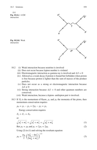
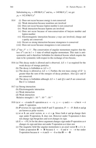
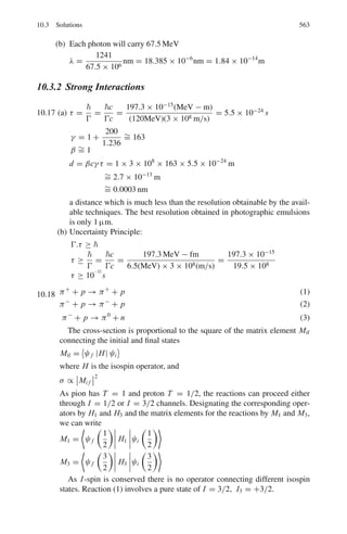
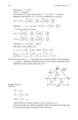
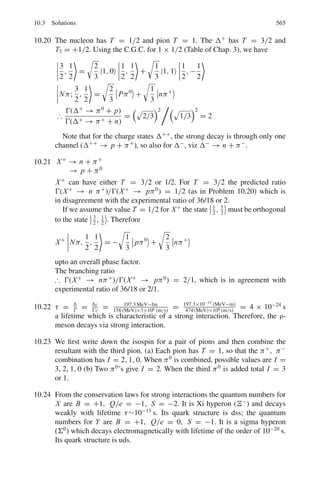
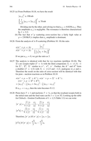
![478 8 Nuclear Physics – II
Writing sin θ∗
dθ∗
= −d(cos θ∗
), and using (3), (4) becomes
5
ln
E1
E2
6
=
E1
0
ln
E1
E2
dE2
E1
= −
ln
E2
E1
dE2
E1
= −
E2
E1
ln
E2
E1
+
E2
E1
%
%
%
%
E1
0
At the upper limit the value is 1. At the lower limit, the second term gives
0. The first term also contributes zero because x ln x in the limit x → 0 gives
zero. Thus,
5
ln
E1
E2
6
= 1.
8.85 (a) The number of collisions required is
n =
1
ξ
ln
E0
En
The average logarithmic energy decrement
ξ = 1 +
(A − 1)2
2A
ln
A − 1
A + 1
For graphite (A = 12), ξ = 0.158
∴ n =
1
0.158
ln
2 × 10⁶
0.025
= 115
(b) Slowing down time
t =
√
2m
ξΣs
[E
−1/2
f − E
−1/2
i ]
∼
=
2mc2/E f
cξΣs
(∵ Ei Ef)
Inserting the values, mc2
= 940 × 106
eV, Ef = 0.025 eV, ξ = 0.158
and Σs = 0.385 cm−1
for graphite, we find the slowing down time t =
1.5 × 10⁻⁴
s.
8.86 If Nu is the number of Uranium atom per cm3
and N0 is the number of 238
U
atoms per cm3
, then N0 = 139
140
Nu. Further, Nm/Nu = 400.
Therefore, Nm/N0 = 400 × 140/139 = 402.9
Thermal utilization factor ( f );
f =
Σa(U)
Σa(U) + Σa(m)
=
Nuσa(U)
Nuσa(U) + Nmσa(m)
=
1
1 + Nmσa(m)
Nuσa(U)
=
1
1 + 402.9×0.0032
7.68
= 0.857](https://image.slidesharecdn.com/1000-solved-problems-in-modern-physics-220626164600-18e7ea67/85/1000-solved-problems-in-modern-physics-pdf-584-320.jpg)
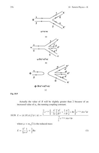
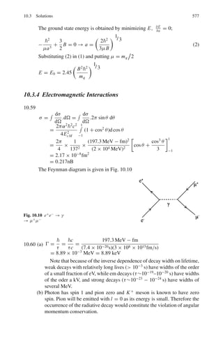
![9.2 Problems 489
Also, calculate the numerical values for the above expressions where α =
1/137 is the fine structure constant. The electron mass is me = 0.511 MeV.
9.4 One of the bound states of positronium has a lifetime given in natural units by
τ = 2/mα5
where m is the mass of the electron and α is the fine structure con-
stant. Using dimensional arguments introduce the factors and c and determine
τ in seconds.
9.5 The V-A theory gives the formula for the width (Γμ) of the muon decay in
natural units.
Γμ = /τ = GF
2
mμ
5
/192π3
Convert the above formula in practical units and calculate the mean life time
of muon
[(GF/(c)3
= 1.116 × 10⁻⁵
GeV−2
, mμ c2
= 105.659 MeV]
9.2.2 Production
9.6 An ultra high energy electron (β ≈ 1) emits a photon. (a) Derive an expression
to express the emission angle θ in the lab system in terms of θ∗
, the angle
of emission in the rest frame of the electron. Also, (b) Show that half of the
photons are emitted within a cone of half angle
θ ≈ 1/γ.
9.7 Show that in a fixed target experiments, the energy available in the CMS goes
as square root of the particle energy (relativistic) in the Lab system.
9.8 A positron with laboratory energy 50 GeV interacts with the atomic electrons
in a lead target to produce μ+
μ−
pairs. If the cross-section for this process is
given by σ = 4πα2
2
c2
/3(ECM)2
, calculate the positron’s interaction length.
The density of lead is ρ = 1.14 × 10⁴
kg m−3
9.9 It is desired to investigate the interaction of e+
and e−
in flight, yielding a
nucleon-antinucleon pair according to the equation of e+
+ e−
→ p + p−
.
(a) To what energy must the positrons be accelerated for the reaction to be
energetically possible in collisions with stationary electrons. (b) How do the
energy requirements change if the electrons are moving, for example in the
form of a high energy beam? (c) What is the minimum energy requirement?
(me c2
= 0.51 MeV, Mp c2
= 938 MeV)
[University of Bristol 1967]
9.2.3 Interaction
9.10 A proton with kinetic energy 200 MeV is incident on a liquid hydrogen target.
Calculate the centre-of-mass energy of its collision with a nucleus of hydro-
gen. What kinds of particles could be produced in this collision?
[University of Wales, Aberystwyth 2003]](https://image.slidesharecdn.com/1000-solved-problems-in-modern-physics-220626164600-18e7ea67/85/1000-solved-problems-in-modern-physics-pdf-595-320.jpg)
![490 9 Particle Physics – I
9.11 Estimate the thickness of iron through which a beam of neutrinos with energy
200 GeV must travel if 1 in 109
of them is to interact. Assume that at high
energies the neutrino-nucleon total cross-section is 10−42
Eν m2
, where Eν is
the neutrino energy is in GeV. The density of iron is 7,900 kg m−3
. [Mass of
nucleon = 1.67 × 10⁻²⁷
kg.]
9.12 (a) The cross-section for scattering of muons with air at atmospheric pressure
is 0.1 barns, and the natural lifetime of muons 2.2 × 10⁻⁶
s. Explain what
is meant by the terms elastic scattering and lifetime. Which of these fac-
tors limits the distance over which a beam of muons can travel in air in a
laboratory, if the muon velocity is 106
ms−1
?
(Assume number density of air at STP = 2.69 × 1025
m−3
)
(b) Given your answer to (a), why is it possible to detect showers of muons at
ground level caused by the impact of primary cosmic ray particles with air
at around 12 km altitude? Given that the mean energy of muons detected
at ground level is ≈ 4 GeV, calculate the distance (in air) over which the
number of such muons in a beam would reduce by a factor of e. What kind
of interactions contribute to the scattering cross-section for these particles?
[1 barn = 10−28
m2
; mass of muon = 105 MeV/c2
; number density of air
at STP = 2.69 × 1025
m−3
]
9.13 Obtain an approximate value for the interaction length (in cm) of a fast proton
in lead from the following data: r0 = 1.3×10⁻¹³
cm, Atomic weight of lead =
207, Density of lead = 11.3 g cm−3
, Avogadro’s number = 6×10²³
molecules
mole−1
[University of Durham 1962]
9.14 A liquid hydrogen target of volume 125 cm3
and density 0.071 g cm−3
is
bombarded with a mono-energetic beam of negative pions with a flux 2 ×
107
m−2
s−1
and the reaction π−
+ p → π0
+ n observed by detecting the
photons from the decay of the π0
. Calculate the number of photons emitted
from the target per second if the cross-section is 40 mb.
9.15 A beam of π+
mesons contaminated with μ+
mesons is passed through an
iron absorber. Given that the interaction cross-section of π+
mesons with
iron is 600 mb/nucleus, calculate the thickness of iron necessary to attenuate
the π+
beam by a factor of 500. Explain why muons will be reduced to a
much less extent. (The density of iron is 7,900 kg m−2
, the atomic mass being
55.85 amu)
9.16 A neutrino of high energy (E0 m) undergoes an elastic scattering with
stationary electron of mass m. The electron recoils at an angle φ with energy
T . Show that for small angle, φ = (2m/T )1/2
9.17 Why the following reactions can not proceed as strong interactions
(a) π−
+ p → K−
+ Σ+
(b) d + d →4
He + π0
?](https://image.slidesharecdn.com/1000-solved-problems-in-modern-physics-220626164600-18e7ea67/85/1000-solved-problems-in-modern-physics-pdf-596-320.jpg)
![9.2 Problems 491
9.18 From the data given calculate the mass of the hyper-fragment ΛHe5
Mass of Λ hyperon is 1115.58 MeV/c2
, Mass of He4
is 3727.32 MeV/c2
Binding energy BΛ for He5
is 3.08 MeV
[University of Dublin 1968]
9.19 Show that for a high energy electron scattering at an angle θ, the value of Q2
is given approximately by
Q2
= 2Ei Ef(1 − cos θ)
where Ei and Ef are the initial and final values of the electron energy and
Q2
is the four-momentum transfer squared. State when this approximation is
justified.
9.2.4 Decay
9.20 Consider the decay process K+
→ π+
π0
with the K+
at rest. Find
(a) the total energy of the π0
meson
(b) its relativistic kinetic energy
The rest mass energy is 494 MeV for K+
, 140 MeV for π+
, 135 MeV for π0
.
9.21 A collimated beam of π-mesons of 100 MeV energy passes through a liquid
hydrogen bubble chamber. The intensity of the beam is found to decrease with
distance s along its path as exp(-as) with a = 9.1×10⁻²
m−1
. Hence calculate
the life time of the π-meson (Rest energy of the π-meson 139 MeV)
[University of Durham 1960]
9.22 One of the decay modes of K+
mesons is K+
→ π+
+ π+
+ π−
. What is the
maximum kinetic energy that any of the pions can have, if the K+
decays at
rest? Given mK = 966.7 me and mπ = 273.2 me
9.23 Show that the energy of the neutrino in the pion rest frame, E
ν, can be written
in natural units as
E
ν =
m2
π − m2
μ
/2mπ
where mπ and mμ are the masses of the charged pion and the muon, respec-
tively. (You may assume here that the neutrino mass is negligible)
[University of Cambridge, Tripos 2004]
9.24 Find the maximum energy of neutron in the decay of Σ+
hyperon at rest via the
scheme, Σ+
→ n +μ+
+νμ. The masses of Σ+
, n, μ+
and νμ are 1,189 MeV,
939 MeV, 106 MeV and zero, respectively.
9.25 A charged kaon, with an energy of 500 MeV decays into a muon and a neu-
trino. Sketch the decay configuration which leads to the neutrino having the
maximum possible momentum, and calculate the magnitude of this value
(mass of charged kaon is 494 MeV/c2
, mass of muon is 106 MeV/c2
)](https://image.slidesharecdn.com/1000-solved-problems-in-modern-physics-220626164600-18e7ea67/85/1000-solved-problems-in-modern-physics-pdf-597-320.jpg)
![492 9 Particle Physics – I
9.26 Heavy mesons, M = 950 me produced in nuclear interactions initiated by a
more energetic beam of π-meson, have an energy of 50 MeV. Their tracks up
to the point of decay have a mean length of 1.7 m. Calculate their mean life
time.
[University of Durham 1960]
9.27 A pion beam from an accelerator target has momentum 10 GeV/c. What frac-
tion of the particles will not have decayed into muons in a pathlength of
100 m?
Out of the pions decays one muon of a 8 GeV/c and a neutrino are produced
at the beginning of the flight path. Assuming that the decay particles follow
the same path, calculate the difference in arrival times at the end of the path.
(Pion mass = 139.6 MeV, muon mass = 105.7 MeV. Mean life time of pion
= 2.6 × 10⁻⁸
s, c = 3 × 10⁸
m s−1
)
[University of Durham 1972]
9.28 Pions in a beam of energy 5 GeV decay in flight. What are the maximum and
minimum energies of the muons from these decays? (mπ = 139.5 MeV/c2
;
mμ = 105.7 MeV/c2
)
9.29 Assuming that a drop in intensity by a factor less than 10 is tolerable, show
that a 1 GeV/c K+
meson beam can be transported over 10 m without a serious
loss of intensity due to decay, while a Λ -hyperon beam of the same momen-
tum after the same distance will not have useful intensity (Take masses of K+
meson and Λ-hyperon to be 0.5 and 1 GeV/c2
, respectively and their lifetimes
10−8
and 2.5 × 10⁻¹⁰
s respectively.
[University of Durham 1970]
9.30 If a particle has rest mass m0 and momentum p, show that the distance traveled
in one lifetime is d = pT0/m0 where T0 is the life time in the frame of
reference in which the particle is at rest.
[University of Dublin 1968]
9.31 A beam of muon neutrinos is produced from the decay of charged pions of
Eπ = 20 GeV. Show that the relationship between the neutrino energy in the
laboratory frame, Eν, and its angle relative to the pion beam θ, for small θ, is
Eν =
Eπ
(1 + γ 2θ2)
=
1 − mμ
2
/mπ
2
where Eπ is the energy of the pion and γ = Eπ /mπ 1
[University of Cambridge, Tripos 2004]
9.32 It is intended to use a charged mono-energetic hyperon beam to perform scat-
tering experiments off liquid hydrogen. Assuming that the beam transport sys-
tem must have a minimum length of 20 m, calculate the minimum momentum
of a Σ beam such that 1% of the hyperons accepted by the transport system
arrive at the hydrogen target (τ = 0.8 × 10⁻¹⁰
s, mΣ = 1.19 GeV/c2
). What](https://image.slidesharecdn.com/1000-solved-problems-in-modern-physics-220626164600-18e7ea67/85/1000-solved-problems-in-modern-physics-pdf-598-320.jpg)
![9.2 Problems 493
measurements would you make to identify the elastic scattering in a (Σ−
p)
collision?
[University of Manchester]
9.33 The energy spectrum for the electrons emitted in muon decay is given by
dω
dEe
=
2G2
F(mμc2
)2
E2
e
(2π)3(c)6
1 −
4Ee
3mμc2
where the electron mass is neglected. Calculate the most probable energy for
the electron. Show on a diagram the orientation of momenta of the decay
product particles and their helicitis when Ee ≈ mμc2
/2. Furthermore, show
the helicity of the muon. Integrate the energy spectrum to find the total
decay width of the muon. Hence compute the muon mean lifetime in seconds
[GF/(c)3
= 1.166 × 10⁻⁵
GeV−2
]
9.34 (a) Explain the following statements. The mean lifetime of the π+
meson is
2.6 × 10⁻⁸
s while that of π0
is 0.8 × 10⁻¹⁶
s.
(b) The π+
and π−
mesons are of equal mass, but the Σ+
and Σ−
baryon
masses differ by 8 MeV/c2
(c) The mean life of the Σ0
baryon is many orders of magnitude smaller than
those of the Λ and Ξ0
baryons.
9.35 In a bubble chamber two tracks originate from a common point, one caused
by a proton of 440 MeV/c and the other one by π−
meson of momentum
126 MeV/c. The angle between the tracks is 64◦
. Determine the mass of the
unknown particle and identify it.
9.2.5 Ionization Chamber, GM Counter and Proportional Counters
9.36 The dead time of a counter system is to be determined by taking measurements
on two radioactive sources individually and collectively. If the pulse counts
over a time interval t are, respectively, N1, N2 and N12, what is the value of
the dead time?
9.37 An ionization chamber is connected to an electrometer of capacitance 0.5 μμ F
and voltage sensitivity of 4 divisions per volt. A beam of α-particles causes a
deflection of 0.8 divisions. Calculate the number of ion pairs required and
the energy of the source of the α-particles (1 ion pair requires energy of
35 eV, e = 1.6 × 10⁻¹⁹
Coulomb)
[Osmania University]
9.38 An ionization chamber is used with an electrometer capable of measuring 7 ×
10−11
A to assay a source of 0.49 MeV beta particles. Assuming saturation
conditions and that all the particles are stopped within the chamber, calculate
the rate at which the beta particles must enter the chamber to just produce a
measurable response. Given the ionization potential for the gas atoms is 35 eV.](https://image.slidesharecdn.com/1000-solved-problems-in-modern-physics-220626164600-18e7ea67/85/1000-solved-problems-in-modern-physics-pdf-599-320.jpg)
![494 9 Particle Physics – I
9.39 Estimate the gas multiplication required to count a 2 MeV proton which gives
up all its energy to the chamber gas in a proportional counter. Assume that the
amplifier input capacitance in parallel with the counter is 1.5×10⁻⁹
F and that
its input sensitivity is 1 mV. Energy required to produce one ion pair is 35 eV.
9.40 Calculate the pulse height obtained from a proportional counter when a 14 keV
electron gives up all its energy to the gas. The gas multiplication factor of the
proportional counter is 600, capacitance of the circuit is 1.0 × 10⁻¹²
F and
energy required to produce an ion pair is 35 eV
9.41 The plateau of a G.M. Counter working at 800 V has a slope of 2.0% count
rate per 100 V. By how much can the working voltage be allowed to vary if the
count rate is to be limited to 0.1%?
9.42 An organic-quenched G.M. tube has the following characteristics.
Working voltage 1,000 V, Diameter of anode 0.2 mm, Diameter of cathode
2.0 cm. Maximum life time 109
counts.
What is the maximum radial field and how long will it last if used for 30 h
per week of 3,000 counts per minute?
[University of New Castle]
9.43 A G.M. tube with a cathode and anode of 2 cm and 0.10 mm radii respectively
is filled with Argon gas to 10 cm Hg pressure. If the tube has 1.0 kV applied
across it, estimate the distance from the anode, at which electron gains just
enough energy in one mean free path to ionize Argon. Ionization potential of
Argon is 15.7 eV and mean free path in Argon is 2 × 10⁻⁴
cm at 76 cm Hg
pressure.
9.44 A S35
containing solution had a specific activity of 1m Curie per ml. A 25 ml
sample of this solution mass was assayed.
(a) in a Geiger-Muller counter, when it registered 2,000 cpm with a back-
ground count of 750 in 5 min; and
(b) in a liquid scintillation counter, where it registered 9,300 cpm with a back-
ground count of 300 in 5 min.
Calculate the efficiency as applied to the measurement of radioactivity and
discuss the factors responsible for the difference in efficiency of these two
types of counters.
[University of Dublin]
9.45 The dead time of a G.M. counter is 100 μs. Find the true counting rate if the
measured rate is 10,000 counts per min.
[Osmania University]
9.46 A pocket dosimeter has a capacitance of 5.0 PF and is fully charged by a
potential of 100 V. What value of leakage resistance can be tolerated if the
meter is not to lose more than 1% of full charge in 1 day?
9.47 A G.M tube with a cathode 4.0 cm in diameter and a wire diameter of 0.01 cm
is filled with argon in which the mean-free-path is 8×10⁻⁴
cm. Given that the](https://image.slidesharecdn.com/1000-solved-problems-in-modern-physics-220626164600-18e7ea67/85/1000-solved-problems-in-modern-physics-pdf-600-320.jpg)
![9.2 Problems 495
ionizing potential for Argon is 15.7 V, calculate the maximum voltage which
must be applied to produce the avalanche.
9.48 An electrometer with a capacitance 0.4 PF and 5.0 PF chamber are both
charged to a potential of 600 V. Calculate the potential of the combined system
after 8 × 10⁹
ions have been collected in the chamber.
9.2.6 Scintillation Counter
9.49 Pions and protons, both with momentum 4 GeV/c, travel between two scintil-
lation counters distance L m apart. What is the minimum value of L necessary
to differentiate between the particles if the time of flight can be measured with
an accuracy of 100 ps?
9.50 In the historical discovery of antiproton, negatively charged particles of pro-
tonic mass had to be isolated from a heavy background of K−
, π−
and μ−
.
The negatively charged particles which originated from the bombardment of a
target with 5.3 GeV protons, were subject to momentum analysis in a magnetic
field which permitted only those particles with momentum p = 1.19 GeV/c
to pass through a telescope system comprising two scintillation counters in
coincidence with a separation of d =12 metres between the detectors. Identify
the particles whose time of flight in the telescope arrangement was determined
as t = 51 ± 1 ns. What would have been the time of flight of π mesons?
9.51 A scintillation spectrometer consists of an anthracene crystal and a 10-stage
photomultiplier tube. The crystal yields about 15 photons for each 1 keV of
energy dissipated. The photo-cathode of the photomultiplier tube generates
one photo-electron for every 10 photons striking it, and each dynode produces
3 secondary electrons. Estimate the pulse height observed at the output of
the spectrometer if a 1 MeV electron deposits its energy in the crystal. The
capacitance of the output circuit is 1.2 × 10⁻¹⁰
F.
9.52 A sodium iodide crystal is used with a ten-stage photomultiplier to observe
protons of energy 5 MeV. The phosphor gives one photon per 100 eV of energy
loss. If the optical collection efficiency is 60% and the conversion efficiency of
the photo-cathode is 5%, calculate the average size and the standard deviation
of the output voltage pulses when the mean gain per stage of the multiplier is
3 and the collector capacity is 12 PF.
[University of Manchester]
9.53 A 400-channel pulse-height analyzer has a dead time τ = (17 + 0.5 K) μs
when it registers counts in channel K. How large may the pulse frequencies
become if in channel 100 the dead time correction is not to exceed 10%?
Repeat the calculations for the channel 400.
9.54 An anthracene crystal and a 12-stage photomultiplier tube are to be used as
a scintillation spectrometer for β-rays. The phototube output circuit has a](https://image.slidesharecdn.com/1000-solved-problems-in-modern-physics-220626164600-18e7ea67/85/1000-solved-problems-in-modern-physics-pdf-601-320.jpg)
![496 9 Particle Physics – I
combined capacitance of 45 PF. If an 8-mV output pulse is desired whenever a
55-keV beta particle is incident on the crystal, calculate the electron multipli-
cation required per stage. Assume perfect light collection and a photo-cathode
efficiency of 5% (assume 550 photons per beta particle)
9.55 Figure 9.1 shows the gamma-ray spectrum of 22
Na in NaI scintillator. Indicate
with explanation the origin of the parts labeled as A, B, C, D and E, Given that
22
Na is a positron emitter and emits a γ -ray of 1.275 MeV.
Fig. 9.1
9.56 Assuming that the shape of the photpeak in the scintillation counter is described
by the normal distribution, show that the half width at half-maximum is
HWHM = 1.177 σ
9.57 The peak response to the 661 keV gamma rays from 137
Cs occurs in energy
channel 298 and 316. Calculate the standard deviation of the energy, and the
coefficient of variation of the energy determination, assuming the pulse ana-
lyzer to be linear.
9.2.7 Cerenkov Counter
9.58 Explain what is meant by Cerenkov radiation. How may a Cerenkov detector
distinguish between a kaon and a pion with the same energy? A pion of energy
20 GeV passes through a chamber containing CO2 at STP. Calculate the angle
to the electron’s path with which the Cerenkov radiation is emitted. (Use the
result that the velocity of a relativistic particle v = c(1 − γ −2
)1/2
. [Mass of
pion = 140 MeV, Mp = 938 MeV; refractive index of CO2 at STP = 1.0004]
9.59 An electron incident on a glass block of refractive index 1.5 emits Cerenkov
radiation at an angle 45◦
to its direction of motion. At what speed is the elec-
tron travelling?
[University of Cambridge, Tripos 2004]
9.60 Consider Cerenkov radiation emitted at angle θ relative to the direction of a
charged particle in a medium of refractive index n. Show that its rest mass
energy mc2
is related to its momentum by mc2
= pc(n2
cos2
θ − 1)1/2](https://image.slidesharecdn.com/1000-solved-problems-in-modern-physics-220626164600-18e7ea67/85/1000-solved-problems-in-modern-physics-pdf-602-320.jpg)
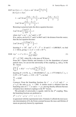
![498 9 Particle Physics – I
9.68 A 10 GeV proton is directed toward the centre of the earth when it is at dis-
tance of 103
earth radius away. Through what mean transverse magnetic field
(assumed uniform) must it move if it is to just miss the earth?
9.69 A proton of kinetic energy 20 keV enters a region where there is uniform elec-
tric field of 500 V/cm, acting perpendicularly to the velocity of the proton.
What is the magnitude of a superimposed magnetic field that will result in no
deflection of the proton?
[University of Manchester]
9.70 A particle of known charge but unknown rest mass is accelerated from rest by
an electric field E into a cloud chamber. After it has traveled a distance d, it
leaves the electric field and enters a magnetic field B directed at right angles
to E. From the radius of curvature of its path, determine the rest mass of the
particle and the time it had taken to traverse the distance d.
[University of Durham]
9.71 A proton accelerated to 500 keV enters a uniform transverse magnetic field of
0.51 T. The field extends over a region of space d = 10 cm thickness. Find
the angle α through which the proton deviates from the initial direction of its
motion.
9.72 An electron is projected up, at an angle of 30◦
with respect to the x-axis, with a
speed of 8 × 10⁵
m/s. Where does the electron recross the x-axis in a constant
electric field of 50 N/C, directed vertically upwards?
9.73 A proton moving with a velocity 3×10⁵
ms−1
enters a magnetic field of 0.3 T,
at an angle of 30◦
with the field. What will the radius of curvature of its path
be (e/m for proton ≈ 108
C kg−1
)?
9.74 What energy must a proton have to circle the earth at the magnetic equator?
Assume a 1 G magnetic field.
9.75 The average flux of primary cosmic rays over earth’s surface is approxi-
mately 1 cm−2
s−1
and their average kinetic energy is 3 GeV. Calculate the
power delivered to the earth from cosmic rays in giga watts. (Earth’s radius
= 6,400 km)
9.76 Kaons with momentum 25 GeV/c and deflected through a collimator slit at a
distance of 10 m from a bending magnet 1.5 m long which produces a field of
1.2 T. What should be minimum width of the slit so that it accepts particles of
momenta within 1% of the central value?
9.2.11 Betatron
9.77 The orbit of electrons in a betatron has a radius of 1m. If the magnetic field
in which the electrons move is changing at the rate of 50 W m−2
s−1
, calculate
the energy acquired by an electron in one rotation. Express your answer in
electron volts.
[University of New Castle 1965]](https://image.slidesharecdn.com/1000-solved-problems-in-modern-physics-220626164600-18e7ea67/85/1000-solved-problems-in-modern-physics-pdf-604-320.jpg)
![9.2 Problems 499
9.78 In a betatron of diameter 72 in operating at 50 c/s the maximum magnetic field
is 1.2 Wb/m2
. Calculate
(a) the number of revolutions made each quarter cycle
(b) the maximum energy of the electrons
(c) the average energy gained per revolution
[University of New Castle 1965]
9.2.12 Cyclotron
9.79 A cyclotron is designed to accelerate protons to an energy of 6 MeV. Deduce
the expression for the kinetic energy in terms of radius, magnetic field etc and
calculate the maximum radius attained.
[University of Bristol 1967]
9.80 If the acceleration potential (peak voltage, 50,000) has a frequency of 1.2 ×
107
c/s, find the field strength for cyclotron resonance when deuterons and
alpha particles, respectively are accelerated. For how long are the parti-
cles accelerated if the radius of orbit at ejection is 30.0 cm? Deuteron rest
mass = 2.01 amu. α-particle rest mass = 4.00 amu
[University of New Castle 1965]
9.81 The original (uniform magnetic field) type of fixed frequency cyclotron was
limited in energy because of the relativistic increase of mass of the accelerated
particle with energy. What percentage increment to the magnetic flux density
at extreme radius would be necessary to preserve the resonance condition for
protons of energy 20 MeV?
[University of Durham 1972]
9.82 A cyclotron is powered by a 50,000 V, 5 Mc/s radio frequency source. If its
diameter is 1.524 m. what magnetic field satisfies the resonance conditions for
(a) protons (b) deuterons (c) alpha-particles? Also what energies will these
particles attain?
[University of Durham 1961]
9.83 In a synchrocyclotron, the magnetic flux density decreases from 15,000 G at
the centre of the magnet to 14,300 G at the limiting radius of 206 cm. Calculate
the range of frequency modulation required for deuteron acceleration and the
maximum kinetic energy of the deuteron. (The rest mass of the deuteron is
3.34 × 10⁻²⁴
g)
[University of London 1959]
9.84 Calculate the magnetic field, B and the Dee radius of a cyclotron which will
accelerate protons to a maximum energy of 5 MeV if a radio frequency of
8 MHz is available.
9.85 When a cyclotron shifts from deuterons to alpha particles it is necessary to
drop the magnetic field slightly. If the atomic masses of 2
H and 4
He are
2.014102 amu and 4.002603 amu, what is the percentage decrease in field
strength that is required?
[Osmania University]](https://image.slidesharecdn.com/1000-solved-problems-in-modern-physics-220626164600-18e7ea67/85/1000-solved-problems-in-modern-physics-pdf-605-320.jpg)
![500 9 Particle Physics – I
9.86 A synchro-cyclotron has a pole diameter of 4 m and a magnetic field of
1.5 W m−2
(15,000 G). What is the maximum energy that can be transmitted
to electrons which are struck by protons extracted from this accelerator?
[University of Bristol 1968]
9.87 If the frequency of the dee voltage at the beginning of an accelerating sequence
is 20 Mc/s, what must be the final frequency if the protons in the pulse have
an energy of 469 MeV?
[University of Durham 1963]
9.2.13 Synchrotron
9.88 At what radius do 30 GeV protons circulate in a synchrotron if the guide field
is 1 W m−2
9.89 Calculate the orbit radius for a synchrotron designed to accelerate protons to
3 GeV assuming a guide field of 14 kG
[University of Durham 1962]
9.90 What percentage depth of modulation must be applied to the dee voltage of
a synchrotron in order to accelerate protons to 313 MeV assuming that the
magnetic field has a 5% radial decrease in magnitude.
[University of Durham 1962]
9.91 An electron synchrotron with a radius of 1 m accelerates electrons to 300 MeV.
Calculate the energy lost by a single electron per revolution when it has
reached maximum energy.
[Andhra University 1966]
9.92 Show that the radius R of the final orbit of a particle of charge q and rest mass
m0 moving perpendicular to a uniform field of magnetic induction B with a
kinetic energy n times its own rest mass energy is given by
R = m0 c (n2
+ 2n)1/2
/qB
9.93 Protons of kinetic energy 50 MeV are injected into a synchrotron when the
magnetic field is 147 G. They are accelerated by an alternating electric field
as the magnetic field rises. Calculate the energy at the moment when the mag-
netic field reaches 12,000 G (rest energy of proton = 938 MeV)
[University of Bristol 1962]
9.94 A synchrotron (an accelerator with an annular magnetic field) accelerates pro-
tons (mass number A = 1) to a kinetic energy of 1,000 MeV. What kinetic
energy could be reached by deuteron (A = 2) or 3
He (A = 3, Z = 2)
when accelerated in this machine? Take the proton mass to be equivalent to
1,000 MeV.
[University of Durham 1970]](https://image.slidesharecdn.com/1000-solved-problems-in-modern-physics-220626164600-18e7ea67/85/1000-solved-problems-in-modern-physics-pdf-606-320.jpg)
![9.2 Problems 501
9.95 A synchrocyclotron accelerates protons to 500 MeV. B = 18 kG, V = 10 kV
and ϕs = 300
. To find
(a) the radius of the orbit at extraction
(b) Energy of ions for acceptance
(c) the initial electric frequency limits
(d) the range of frequency modulation
9.96 Explain how a synchrotron accelerates particles. What is the main energy loss
mechanism in these devices? How much more power is needed to maintain a
beam of 500 GeV electrons in a synchrotron of radius 1 km than to maintain a
beam of protons of the same energy? Is this feasible?
[University of Aberyswyth 2003]
9.97 Protons are accelerated in a synchrotron in the orbit of 10 m. At one moment in
the cycle of acceleration, protons are making one revolution per microsecond.
Calculate the value at this moment of the kinetic energy of each proton in MeV.
[University of Bristol 1961]
9.98 Electrons are accelerated to an energy of 10 MeV in a linear accelerator, and
then injected into a synchrotron of radius 15 m, from which they are acceler-
ated with an energy of 5 GeV. The energy gain per revolution is 1keV
(a) Calculate the initial frequency of the RF source. Will it be necessary to
change this frequency?
(b) How many turns will the electron make?
(c) Calculate the time between injection and extraction of the electrons
(d) What distance do the electrons travel within the synchrotron?
9.2.14 Linear Accelerator
9.99 Protons of 2 MeV energy enter a linear accelerator which has 97 drift tubes
connected alternately to a 200 MHz oscillator. The final energy of the pro-
tons is 50 MeV (a) What are the lengths of the second cylinder and the last
cylinder (b) How many additional tubes would be needed to produce 80 MeV
protons in this accelerator?
9.100 The Stanford linear accelerator produces 50 pulses per second of about 5 ×
1011
electrons with a final energy of 2 GeV. Calculate (a) the average beam
current (b) the power output.
9.101 A section of linear accelerator has five drift tubes and is driven by a 50 Mc
oscillator. Assuming that the protons are injected into the first drift tube at
100 kV and gain 100 kV in every gap crossing
(a) What is the output energy after the fifth drift tube?
(b) What is the total length of the whole section? (Ignore the gap length)
[AEC 1966 Trombay]](https://image.slidesharecdn.com/1000-solved-problems-in-modern-physics-220626164600-18e7ea67/85/1000-solved-problems-in-modern-physics-pdf-607-320.jpg)
![502 9 Particle Physics – I
9.102 What is the length L of the longest drift tube in a linac which operating at a
frequency of f = 25 MHz is capable of accelerating 12
C ions to a maximum
energy of E = 80 MeV?
9.2.15 Colliders
9.103 Two beams of particles consisting of n bunches with N1 and N2 particles
in each circulate in a collider and make head-on-collisions. A, the cross-
sectional area of the beam and f is the frequency with which the particles
circulate, obtain an expression for the luminosity L.
9.104 In an electron-positron collider the particles circulate in short cylindrical
bunches of radius 1.2 mm. The number of particles per bunch is 6 ×10¹¹
and
the bunches collide at a frequency of 2 MHz. The cross-section for μ+
μ−
creation at 8 GeV total energy is, 1.4 × 10⁻³³
cm2
; how many μ+
μ−
pairs
are created per second?
9.105 (a) Show that in a head-on-collision of a beam of relativistic particles of
energy E1 with one of energy E2, the square of the energy in the CMS is 4
E1 E2 and that for a crossing angle θ between the beam this is reduced by
a factor (1+cos θ)/2, (neglect the masses of beam particles in comparison
with the energy)
(b) Show that the available kinetic energy in the head-on-collision with two
25 GeV protons is equal to that in the collision of a 1,300 GeV proton with
a fixed hydrogen target. (Courtesy D.H. Perkins, Cambridge University
Press)
9.106 Head-on collisions are observed between protons each moving with velocity
(relative to the fixed observer) corresponding to 1010
eV. If one of the protons
were to be at rest relative to the observer, what would the energy of the other
need to be so as to produce the same collision energy as before. The rest
energy of the proton is 109
eV.
[University of Manchester 1958]
9.107 It is required to cause protons to collide with an energy measured in their
centre of mass frame, of 4 M0c2
in excess of their rest energy 2 M0c2
. This
can be achieved by firing protons at one another with two accelerators each of
which imparts a kinetic energy of 2 M0c2
. Alternatively, protons can be fired
from an accelerator at protons at rest. How much energy must this single
machine be capable of imparting to a proton? What is the significance of this
result for experiments in high energy nuclear physics?
[University of New Castle 1966]
9.108 The HERA accelerator in Hamburg provided head-on collisions between
30 GeV electrons and 820 GeV protons. Calculate the centre of mass energy
that was produced in each collision.
[Manchester 2008]](https://image.slidesharecdn.com/1000-solved-problems-in-modern-physics-220626164600-18e7ea67/85/1000-solved-problems-in-modern-physics-pdf-608-320.jpg)
![9.3 Solutions 503
9.109 At a collider, a 20 GeV electron beam collides with a 300 GeV proton beam at
a crossing angle of 10◦
. Evaluate the total centre of mass energy and calculate
what beam energy would be required in a fixed-target electron machine to
achieve the same total centre-of-mass energy.
9.3 Solutions
9.3.1 System of Units
9.1 E = Mc2
= 1 × (3 × 108
)2
= 9 × 10¹⁶
J
= 9 × 10¹⁶
J/(1.6 × 10−10
J/GeV) = 5.63 × 1026
GeV
9.2 (a) c = 197.3 MeV-fm
In natural units, = c = 1
Therefore 1 = 197.3 MeV-fm = 0.1973 GeV-10−15
m
Therefore 10−15
m = 1/0.1973 GeV−1
or 1 m = 1015
/0.1973 = 5.068 × 10¹⁵
GeV−1
(b) From (a) we have
1 m2
= (5.068)2
× 1030
GeV−2
= 25.6846 × 1030
GeV−2
Therefore 1 GeV−2
= 10−30
/25.6846 m2
= 0.389 mb
(c) = 1.055 × 10⁻³⁴
J-s
1 = 1.055 × 10⁻³⁴
J-s/1.6 × 10−10
J/GeV
Therefore 1 s = (1.6 × 10⁻¹⁰
/1.055 × 10−34
) GeV−1
= 1.5 × 1024
GeV−1
9.3 (a) In practical units λc = /me c
Put = c = 1
In natural units λc = 1/me
(b) In practical units Bohr’s radius of hydrogen atom is
a0 = ε0 2
/π me2
= ε0 c/πm ce2
In natural units a0 = 1/αme
(c) In the ground state velocity
v = /ma0 = α
where we have used the results of (b)
Put = 1 to find v = α in natural units.
Numerical values:
λc = /mec = (c/mec2
) MeV.fm/MeV = 197.3/0.511 fm = 385 fm
= 0.00385 × 10⁻¹⁰
m
= 0.00385 Å
a0 = 4πε0 2
/e2
m = (4 πε0/e2
) ( c)2
/mc2
= [1/(1.44 MeV-fm)] × (197.3 MeV-fm)2
/0.511 MeV
= 53,000 fm = 0.53 × 10⁻¹⁰
m
v = αc = (3 × 10⁸
/137) ms−1
= 2.19 × 10⁶
ms−1](https://image.slidesharecdn.com/1000-solved-problems-in-modern-physics-220626164600-18e7ea67/85/1000-solved-problems-in-modern-physics-pdf-609-320.jpg)
![504 9 Particle Physics – I
9.4 In natural units τ = 2/mα5
. Introduce the factors and c
Let τ = 2x
cy
/m α5
Find the dimensions: [] = [Energy × Time], [c] = [velocity]
[τ] = [1/m][ML2
T−1
]x
[LT−1
]y
[T] = [M]x−1
[L]2x+y
[T]−x−y
Equating the coefficients on both sides of the equation,
−x − y = 1, 2x + y = 0, x − 1 = 0
we get x = 1, y = −2
Therefore τ = 2c−2
/mα5
= 2 /mc2
α5
τ = 2 × (0.659 × 10−21
MeV-s) × (137)5
/0.511 MeV
= 1.245 × 10⁻¹⁰
s
9.5 Γμ = GF
2
mμ
5
/192π3
(1)
Now, the dimensional formula for GF is
[Energy]−2
[ c]3
and [Γμ] = [Energy]
Introduce and c in (1) and take dimensions on both sides.
Γμ = GF
2
mμ5
x
cy
/192π3
(2)
[M L2
T−2
] = [M L2
T −2
]−4
[M]5
[M L2
T −1
]x+6
[L T−1
]y+6
or [M L2
T −2
] = [M]7+x
[L]10+2x+y
[T ]−4−x−y
Equating powers of M, L and T , we find
x = −6 and y = 4
and (2) becomes
Γμ = GF
2
mμ
5
−6
c4
/192π3
Γμ = /τ = GF
2
(mμc2
)5
/192 (c)6
π3
= (1.116 × 10⁻⁵
GeV−2
)2
(105.659 × 10⁻³
)5
/192π3
τ = 2.39 × 10⁻⁶
s
9.3.2 Production
9.6 (a) The relation for lab angle θ and the C.M.S. angle θ∗
is given by
tan θ = sin θ∗
/γc(cos θ∗
+ βc/β∗
) (1)
where βc = vc/c is the CMS velocity and γc is the corresponding Lorentz
factor (see summary of Chap. 6). For photon β∗
= 1 and βc = 1 as the
electron is ultra relativistic. Dropping off the subscript c, (1) becomes
tan θ = sin θ∗
/γ (cos θ∗
+ 1) = tan (θ∗
/2)/γ (2)
(b) Assuming that the photons are emitted isotropically, half of the photons will
be contained in the forward hemisphere in the CMS, that is within θ∗
= 90◦
.
Substituting θ∗
= 90◦
in (2)
tan θ = 1/γ
As the incident electron is ultrarelativistic the photons in the lab would come
off at small angles so that tan θ ≈ θ = 1/γ . Thus half of the photons will be
emitted within a cone of half angle θ ≈ 1/γ .](https://image.slidesharecdn.com/1000-solved-problems-in-modern-physics-220626164600-18e7ea67/85/1000-solved-problems-in-modern-physics-pdf-610-320.jpg)
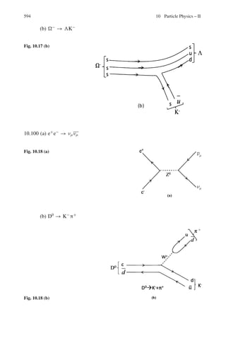
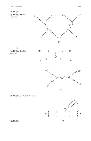
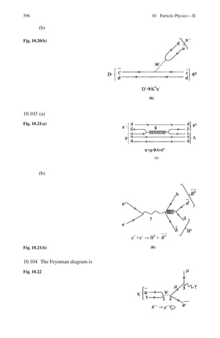
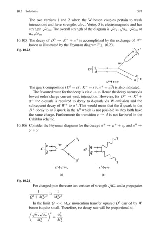
![9.3 Solutions 509
En =
mΣ
2
+ mn
2
− mμ
2
/2mΣ = (1,1892
+ 9392
− 1062
)/2 × 1,189 =
960.6 MeV
Therefore Tn = En − mn = 960.6 − 939 = 21.6 MeV
9.25 Maximum neutrino momentum in the L-system is obtained when the neutrino
is emitted in the forward direction, that is at θ∗
= 0 in the rest system of
K-meson (Fig. 9.3).
The energy of the neutrino in the rest frame of K-meson is
Eν
∗
=
mK
2
− mμ
2
/2mK = 235.6 MeV
Pν
∗
= 235.6 MeV/c (because mν = 0)
Pν = γK pν
∗
(1 + βKβν
∗
cos θ∗
)
βν
∗
= 1; θ∗
= 0; pν
∗
= 235.6 MeV/c
γK = 1 + TK/mK = 1 + 500/494 = 2.012
βK = 0.868
pν = (2.012)(235.6)(1 + 0.868) = 885.5 MeV/c
Fig. 9.3 Decay configuration
9.26 Rest mass energy of the heavy meson, M = 965 × 0.511 = 493 MeV
γ = 1 + T/M = 1 + 50/493 = 1.101
β = (γ 2
− 1)1/2
/γ = (1.1012
− 1)1/2
/1.101 = 0.418
Observed mean lifetime τ is related to proper lifetime by
τ = τ0γ
τ = d/βc = 1.7/0.418 × 3 × 108
= 1.355 × 10⁻⁸
s = 1.101 τ0
Therefore τ0 = 1.23 × 10⁻⁸
s
9.27 Fraction of pions that will not decay
I/I0 = exp(−t/τ0) = exp(−d/β c γ τ0)
γ = E/m = (p2
+ m2
)1/2
/m = [(p2
/m2
) + 1]1/2
= [(10/0.1396)2
+ 1]1/2
=
71.64
β ≈ 1
Therefore I/I0 =exp(−100/1×3×108
×71.64×2.6×10−8
)= exp(−0.179) =
0.836
γμ = ((p2
/m2
) + 1)1/2
= ((82
/0.10572
) + 1)1/2
= 75.69
βμ ≈ 1
tμ = dγ/βc = 100 × 75.69/1 × 3 × 108
= 25.23 × 10⁻⁶
s
tν = d/c = 100/3 × 108
= 0.333 × 10⁻⁶
s
Therefore Δt = tμ − tν = (25.23 − 0.33) × 10−6
s
= 24.9 μs
9.28 In the rest system of pion the muon is emitted with kinetic energy
Tμ
∗
= 4 MeV (see Problem 6.54)
Its energy in the LS will be maximum when θ∗
= 0 and minimum when
θ∗
= 180 in the CMS. Applying the relativistic transformation equation](https://image.slidesharecdn.com/1000-solved-problems-in-modern-physics-220626164600-18e7ea67/85/1000-solved-problems-in-modern-physics-pdf-615-320.jpg)
![510 9 Particle Physics – I
Eμ = Eμ
∗
γπ (1 + βμ
∗
βπ cos θ∗
)
Eμ
∗
= 105.7 + 4.0 = 109.7 MeV; γμ
∗
= 1.0378; βμ
∗
= 0.2676
γπ = 5/0.1395 = 35.84; βπ ≈ 1
Eμ (max) = 4.98 GeV; Eμ (min) = 2.88 GeV
9.29 The decay equation is
I = I0 exp (−t/γ τ) = I0 exp(−d/β c γ τ) (1)
For K+
meson beam
βK = 1/
,
1 + mK
2
/pK
2
-1/2
Substituting mK = 0.5 GeV/c2
and pK = 1 GeV/c
βK = 0.894; γK = 2.23; τK = 10−8
s; d = 10 m
Using these values in Eq. (1)
I/I0 = exp(−1.672) = 0.188
which is tolerable.
For Λ-hyperon beam
βΛ = 1/
,
1 + mΛ
2
/pΛ
2
-1/2
= 0.7
γΛ = 1.96, τΛ = 2.5 × 10⁻¹⁰
s; d = 10 m
Using the above values in (1) we find
I/I0 = exp(−97) ≈ zero
which is not at all useful.
9.30 d = vt (1)
t = γ T0 (2)
p = m0 v γ (3)
Combining (1), (2) and (3)
d = pT0/m0
9.31 Inverse Lorentz transformations gives
Eν
∗
= γ Eν(1 − β cos θ) = Eν[γ − (γ 2
− 1)1/2
cos θ]
= Eν[γ − γ (1 − 1/2γ 2
)(1 − θ2
/2)]
Eν
∗
≈ (Eν/2γ )(1 + γ 2
θ2
) (1)
where we have neglected terms θ2
/2γ for γ 1 and considered small θ.
But Eν
∗
=
mπ
2
− mμ
2
/2mπ and Eπ = γ mπ (2)
Using (2) in (1) we get the desired result.
9.32 I/I0 = 1/100 = exp(−d/βc γ τ)
Put d = 20 m, c = 3 × 10⁸
m/s and τ = 0.8 × 10⁻¹⁰
s and take loge on
both sides to solve for βγ . We find βγ = 181. Therefore, the momentum of
hyperon,
cp = mβγ = 1.19 × 181 = 215 GeV
Thus, the minimum momentum required is P = 215 GeV/c
The elastic scattering of Σ−
hyperons with protons can be recorded in the
hydrogen bubble chamber from the kinematical fits of events.](https://image.slidesharecdn.com/1000-solved-problems-in-modern-physics-220626164600-18e7ea67/85/1000-solved-problems-in-modern-physics-pdf-616-320.jpg)
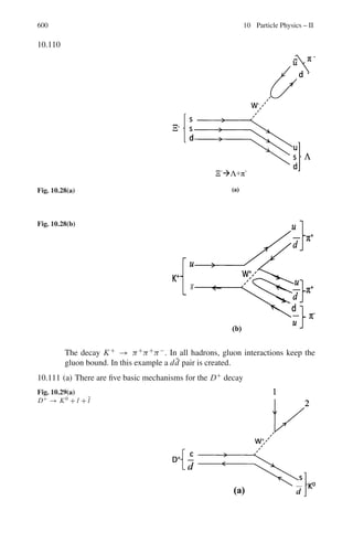
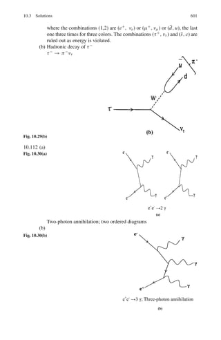
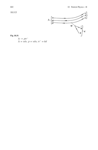
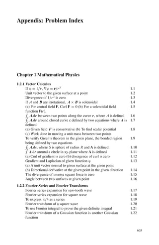
![9.3 Solutions 515
where τ is the dead time. τ = 100 μs = 10−4
s.
n0 = 104
/ min = 166.7/s
n = (104
/ min)/(1 − 166.7 × 10⁻⁴
) = 10,169/ min
9.46 V = V0 e−t/RC
et/RC
= V0/V = 100/99
R = t/C ln(100/99) = 86,400/(5 × 10−12
)(0.01) = 1.73 × 10¹⁸
ohm.
9.47 V = Er ln(d1/d2) (1)
Put r = d2/2 = 0.01/2 = 0.005 cm
E = 15.7/λ = 15.7/8 × 10−4
V/cm = 19,625 V/cm
d1/d2 = 4/0.01 = 400
V = (19,625)(0.005) ln 400 = 588 V.
9.48 Q = CV
Initial chamber charge:
Qch = 5 × 10−12
× 600 = 3.0 × 10⁻⁹
Coulomb
Initial electrometer charge:
Qel = 0.4 × 10−12
× 600 = 0.24 × 10⁻⁹
Coulomb
Chamber charge lost:
8 × 109
× 1.6 × 10−19
= 1.28 × 10⁻⁹
Coulomb
Final chamber charge:
Qch
(3.0 − 1.28) × 10−9
= 1.72 × 10⁻⁹
Final electrometer charge:
Q
el = 0.24 × 10⁻¹⁹
Coulomb
Final system charge
Q = (1.72 + 0.24) × 10−9
= 1.96 × 10⁻⁹
Coulomb
Total capacitance C = (5.0 + 0.4) × 10−12
F = (5.4 × 10⁻¹²
)
Final potential= 1.96 × 10⁻⁹
/5.4 × 10−12
= 363 V .
9.3.6 Scintillation Counter
9.49 The velocity of a particle
β = p/E = p/(p2
+ m2
)1/2
The time taken to cross a distance L is
t = L/βc = (L/c)[(p2
+ m2
)/p2
]1/2
= (L/c)[(1 + (m2
/p2
)]1/2
The difference in time taken for proton and pion is
Δt = tp − tπ = (L/c)
.,
1 +
mp
2
/p2
-1/2
−
,
1 +
mπ
2
/p2
-1/2
/
Substituting, Δt = 100 × 10−12
s, c = 3 × 10⁸
ms−1
mp = 0.94 GeV/c2
, mπ = 0.14 GeV/c2
and p = 4 GeV/c, and solving for
L, we find the minimum value of L = 1.14 m
9.50 t =
d
c
1 +
m2
p2
1/2
Put t = 51 × 10−9
s, c = 3 × 10⁸
m/s, d = 12 m and p = 1.19 GeV/c and
solve for m to find m p− = 0.94 GeV/c2
for the anti proton mass.](https://image.slidesharecdn.com/1000-solved-problems-in-modern-physics-220626164600-18e7ea67/85/1000-solved-problems-in-modern-physics-pdf-621-320.jpg)
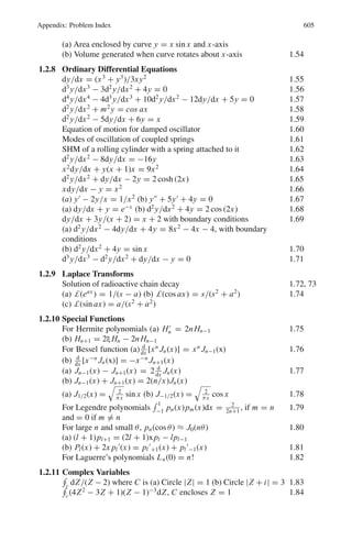
![9.3 Solutions 517
9.55 Label A is due to photopeak of 1.275 MeV γ -rays. Some of the primary pho-
tons will be absorbed within the crystal after undergoing Compton scattering.
Such events merely enhance the photopeak. In other cases, the Compton-
scattered photon will escape from the crystal, the light output will now be
proportional to the energy of the recoil electron which will be absorbed in a
large crystal. There will be a energy continuum of the recoil electrons with
energy ranging from zero to maximum. The label B represents the Compton
shoulder. The strong peak labeled C marks the photopeak at 0.511 MeV due
to electron-positron annihilation leading to absorption of one of the photons.
The annihilation may take place from the positron emitted by the source or
by the pair production caused by the primary photon. Now the total kinetic
energy available by the electron-positron pair will be (hν − 1.02) MeV. When
all of the energy is dissipated, the positron will be annihilated. If both the
annihilation photons escape from the crystal, a peak (called Escape peak) will
occur at an energy (hν−1.02) MeV = 1.275−1.02 = 0.255 MeV, represented
by label D. If one of the photons escapes, another peak will occur at an energy
(hν −0.511) MeV = 1.275−0.511 = 0.764 MeV (not shown in the Fig. 9.6).
If both the photons are absorbed, full output will be realized and this will be
added up to the photo peak.
Fig. 9.6
If the annihilation peak at 0.511 MeV and the photo peak due to primary
photon occur simultaneously within the resolving time of the instrument then
their energies are added and the events are recorded as a single event, known
as sum peak at energy 1.275 + 0.511 = 1.786 MeV (label E), usually with
small amplitude.
9.56 The normal distribution is
p(x) =
σ
√
2π
−1
exp[−(x̄ − x)/2σ2
] (1)](https://image.slidesharecdn.com/1000-solved-problems-in-modern-physics-220626164600-18e7ea67/85/1000-solved-problems-in-modern-physics-pdf-623-320.jpg)
![9.3 Solutions 527
E = (p2
+ m2
)1/2
= (9002
+ 9382
)1/2
= 1, 300 MeV
γ = 1, 300/938 = 1.386
β = 0.692
Maximum energy transferred to electron is
E(max) = 2mβ2
γ 2
= 2 × 0.511 × 0.6922
× 1.3862
= 0.94 MeV
9.87 Initially ω0 = qB/m
ω = qB/mγ = ω0/γ
γ = 1 + T/m = 1 + 469/938 = 1.5
f = f0/γ = 20/1.5 = 13.33 Mc/s
9.3.13 Synchrotron
9.88 P = 0.3 BR
P = (T 2
+ 2 Tm)1/2
= (302
+ 2 × 30 × 0.938)1/2
= 30.924 GeV/c
R = p/0.3 B = 30.924/0.3 × 1 = 103.08 m
9.89 p = 0.3 BR
P = (T2
+ 2Tm)1/2
= [32
+ (2 × 3 × 0.938]1/2
= 3.825 GeV/c
R = p/0.3 B = 3.825/(0.3 × 1.4) = 9.1 m
9.90 Initially ω0 = B0 e/m
Finally ω = 0.95 B0 e/(m + T )
ω/ω0 = 0.95m/(m + T )
ω0 − ω
ω0
=
T + 0.05 m
T + m
=
313 + 0.05 × 938
313 + 938
= 0.288
Therefore Depth of modulation is 28.8 %
9.91 Radiation loss per revolution
ΔE = (4π e2
/3R)(E/mc2
)4
.1/4 πε0
= (1.44 × 4π/3R)(E/mc2
)4
MeV-fm
Substituting E = 300 MeV, mc2
= 0.511 MeV
R = 1.0 × 10¹⁵
fm
ΔE = 716 × 10−6
MeV = 716 eV
9.92 p = qBR
R = p/qB = m0γβ c/qB = m0 c (γ 2
− 1)1/2
/qB
But γ = (T/m0c2
) + 1 = n + 1
∴ γ 2
− 1 = n2
+ 2n
∴ R = (m0 c/qB)(n2
+ 2n)1/2](https://image.slidesharecdn.com/1000-solved-problems-in-modern-physics-220626164600-18e7ea67/85/1000-solved-problems-in-modern-physics-pdf-633-320.jpg)
![528 9 Particle Physics – I
9.93 Using the result of Problem 9.92
R =
m0c
qB
(n2
+ 2n)
1
2
=
m0c
0.0147q
50
940
2
+
2 × 50
940
'1/2
= 22.48
m0c
q
(1)
As the radius of synchrotron does not change, we can use the same relation at
higher energy
R =
m0c
1.2q
(N2
+ 2N)1/2
(2)
Combining (1) and (2) and solving for n, we find N = 26
∴ T = Nm0 c2
= 26 × 0.938 = 24.39 GeV
9.94 Using the results of Problem 9.92
q/m0 = (c/BR)(n2
+ 2n)1/2
(1)
Proton: q/m0 = 1/1 = 1
n = T/mp = 1,000/1,000 = 1
Using the above values in (1)
c/BR = 1/
√
3 (2)
Deuteron: q/m0 = 1/2
Therefore 1/2 = (n2
+ 2n)1/2
/
√
3
Solving for n, we find n = 0.3229
Kinetic energy of deuteron = nmd
= 0.3229 × 2,000 MeV
= 646 MeV
3
He : q/m0 = 2/3
Therefore 2/3 = (1/
√
3)(n2
+ 2n)1/2
Solving for n, we find n = 0.527
Therefore Kinetic energy of 3
He = nmHe3
= 0.527 × 3, 000 MeV
= 1, 583 MeV.
9.95 (a) p = 0.3 BR (GeV/c if B is in Tesla and R in metres)
P = (T 2
+ 2T mc2
)1/2
= (0.52
+ 2 × 0.5 × 0.938)1/2
= 1.09 GeV/c
B = 18 kG = 1.8 T
R = p/0.3 B = 1.09/(0.3 × 1.8) = 2.02 m.
(b) Energy of ions for acceptance
Ts = ±(2eV.mc2
/π)1/2
[(ϕs − π/2) sin ϕs + cos ϕs]1/2
(1)
Substitute in (1), 10 keV = 0.01 MeV
mc2
= 938 MeV; ϕs = 300
= 0.5236 radians
Ts = ±2.5 MeV
(c) The initial frequency
f = Bqc2
/2π (mc2
+ Ts) (2)](https://image.slidesharecdn.com/1000-solved-problems-in-modern-physics-220626164600-18e7ea67/85/1000-solved-problems-in-modern-physics-pdf-634-320.jpg)
![530 9 Particle Physics – I
9.98 (a) At injection γ = 1 + 10
0.511
= 20.57
β = 0.9988
At extraction γ = 1 + 5,000
0.511
= 9, 786
β ≈ 1
Initial frequency f1 =
βc
2πr
=
(0.9988) × 3 × 108
2π × 15
c = 3.1809 Mc
Final frequency f2 =
1 × 3 × 108
2π × 15
= 3.1847 Mc
As the initial and final frequencies are nearly the same there is hardly
any need to change the R.F. frequency.
(b) Total energy gain= Ef − Ei = 5,000 − 10 = 4,990 MeV
Energy gain per turn = 1 keV
∴ Number of turns, n = 4,990
10−3 = 4.99 × 10⁶
(c) The period of revolution
T0 = 1/f = 1/3.18 × 106
= 3.14 × 10⁻⁷
s
Time between injection and extraction is
T = nT0 = 4.99 × 106
× 3.14 × 10−7
= 1.567 s
(d) The total distance traveled by the electron is
d = 2πrn = 2π × 15 × 4.99 × 106
= 4.7 × 10⁸
m = 4.7 × 10⁵
km.
9.3.14 Linear Accelerator
9.99 (a) As there are 97 drift tubes, there will be 96 gaps. The energy gain per
gap is ΔE = (50–2)/96 = 0.5 MeV/gap
After crossing the first gap, the protons are still non-relativistic and
their velocity will be in the second drift tube will be
v2 = (2T/m)1/2
= c [2 × (2 + 0.5)/938]1/2
= 0.073 c
The length of the second tube
l2 = v2/2 f = (0.073 × 3 × 1010
/2 × 2 × 108
) cm
= 5.48 cm
In the last tube v is calculated relativistically.
γ = 1 + T/m = 1 + 50/938 = 1.053
β = (γ 2
− 1)1/2
/γ = 0.313
lf = βc/2 f = 0.313 × 3 × 1010
/2 × 2 × 108
= 23.48 cm
(b) To produce 80 MeV protons, number of additional tubes required is (80−
50)/0.5 = 60
9.100 (a) Beam current i = q/t = 50 × 5 × 1011
× 1.6 × 10−19
= 4 × 10⁻⁶
amp
= 4μA](https://image.slidesharecdn.com/1000-solved-problems-in-modern-physics-220626164600-18e7ea67/85/1000-solved-problems-in-modern-physics-pdf-636-320.jpg)
![9.3 Solutions 533
9.108 The CMS energy is calculated from the invariance of E2
− p2
E∗2
= E2
− p2
=
Ep + Ee
2
−
pp − pe
2
= E2
p − p2
p + E2
e − p2
e + 2
Ep Ee + pp pe
≈ mp
2
+ me
2
+ 4Ep Ee
Since mp Ep and me Ee
E∗
≈
4Ep Ee =
√
4 × 820 × 30 = 314 GeV
Note that the HERA accelerator is different from other colliders in that the
energy of the colliding particles (protons and electrons) is quite asymmet-
rical. It has been possible to achieve high momentum transfer in the CMS
(20,000 GeV2
), necessary for the studies of proton structure.
9.109 Total CMS energy, E∗
≈ [2 E1 E2 (1 + cos θ)/2]1/2
Substituting E1 = 20 GeV, E2 = 300 GeV, and θ = 100
we find E∗
= 109 GeV
If the same energy (E∗
= 109 GeV) is to be achieved in a fixed target
experiment, then the electron energy in the lab-system would be
(2 E M + M2
+ m2
)1/2
= E∗
Neglecting M2
and m2
E = (E∗
)2
/2M = (109)2
/(2 × 0.94) ≈ 6, 300 GeV](https://image.slidesharecdn.com/1000-solved-problems-in-modern-physics-220626164600-18e7ea67/85/1000-solved-problems-in-modern-physics-pdf-639-320.jpg)

![544 10 Particle Physics – II
matrix element, the general form being (q2
+ m2
)−1
, where m is the mass of the
exchanged particle and q is the four-momentum transfer.
In general, the same end result is obtained from a number of Feynman diagrams.
The transition matrix element includes the superposition of amplitudes of all such
diagrams.
For the weak interaction the exchanged particle is a massive boson, W±
or Z0
,
indicated by a wavy or broken line. For the strong interaction, the exchanged particle
is a gluon indicated by a spring.
10.2 Problems
10.2.1 Conservation Laws
10.1 Are the following particle interactions allowed by the conservation
rules? If so, state which force is involved and draw a Feynman diagram for
the process.
[University of Aberystwyth 2003]
(i) μ−
→ e−
+ νμ + νe
(ii) Λ → π+
+ π−
(iii) νe + n → p + e−
(iv) π0
→ τ+
+ τ−
(v) e+
+ e−
→ μ+
+ μ−
10.2 Indicate, with an explanation, whether the following interactions proceed
through the strong, electromagnetic or weak interactions, or whether they
do not occur.
(i) π−
→ μ−
+ νμ
(ii) τ−
→ μ−
+ ντ
(iii) Σ0
→ Λ + γ
(iv) p → n + e+
+ νe
(v) π−
+ p → π0
+ Σ0
(vi) π−
+ p → K0
+ Σ0
(vii) e+
+ e−
→ μ+
+ μ−
10.3 Consider the decay of K0
meson of momentum P0 into π+
and π−
of
momenta p+ and p− in the opposite direction such that p+ = 2p−. Deter-
mine p0.
[Mass of K0
is 498 MeV/c2
; mass of π±
is 140 MeV/c2
]
10.4 Indicate, with an explanation, whether the following interactions proceed
through the strong, electromagnetic or weak interactions, or whether they
do not occur.
(i) Ξ−
→ Σ−
+ π0
(ii) τ−
→ e−
+ νe + ντ
(iii) τ+
→ μ+
+ γ](https://image.slidesharecdn.com/1000-solved-problems-in-modern-physics-220626164600-18e7ea67/85/1000-solved-problems-in-modern-physics-pdf-650-320.jpg)


![ANIMAL_CELL_,_TISSUE_AND_ORGAN_CULTURE[1].pptx](https://cdn.slidesharecdn.com/ss_thumbnails/animalcelltissueandorganculture1-260204172026-4462b440-thumbnail.jpg?width=640&height=640&fit=bounds)


