Download as PDF, PPTX

![3
Key Concepts - Scale
[1]
Neighbourhood
(1-2km)
Street Canyon
(up to 200m)
City
(10-20km)
Regional
(100-200km)](https://image.slidesharecdn.com/rosiedavies-180424125706/85/Advanced-Gaussian-Model-or-CFD-3-320.jpg)
![4
Key Concepts – Urban Topology and ABL
[2]
• Near Field vs Far Field ?](https://image.slidesharecdn.com/rosiedavies-180424125706/85/Advanced-Gaussian-Model-or-CFD-4-320.jpg)
![5
Key Concepts – Turbulence
• Turbulence is typically greater in urban areas than in rural locations due to higher
surface roughness, traffic movement and urban heat island effect (20-50% greater [3])
• Higher turbulence in urban areas will increase plume dilution and decrease maximum
ground level concentration, compared to that measured in an open country exposure
(dilution increased 2x [4])
Image from [2].](https://image.slidesharecdn.com/rosiedavies-180424125706/85/Advanced-Gaussian-Model-or-CFD-5-320.jpg)
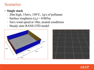
![8
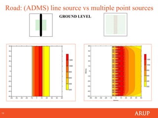
• Road
- Based on CEDVAL experiment [5] without the pitched roof
- Road width = 20m with 1g/km/s of pollutant
- Canyon height = 20m
- Building = 100m x 100m x 20m
Scenarios](https://image.slidesharecdn.com/rosiedavies-180424125706/85/Advanced-Gaussian-Model-or-CFD-8-320.jpg)


![20
• [1] “A review on the CFD analysis of urban microclimate” – Toparrlar et al.,
2017
• [2] “On the use of numerical modelling for near field pollutant dispersion in
urban environment” – Lateb et al., 2015
• [3] “Recent progress in CFD modelling of wind field and pollutant transport
in street canyons” – XL Li et al., 2016
• [4] “Ten questions concerning modelling of near-field pollutant dispersion in
the built environment” – Y.Tominaga and T.Stathopoulos, 2016
• [5] “Flow and Pollutant Dispersion in Street Canyons using FLUENT and
ADMS-Urban” – Di Sabatino et al., 2008
References](https://image.slidesharecdn.com/rosiedavies-180424125706/85/Advanced-Gaussian-Model-or-CFD-20-320.jpg)

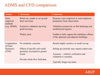
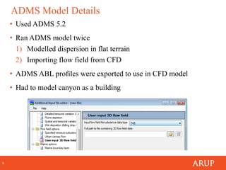
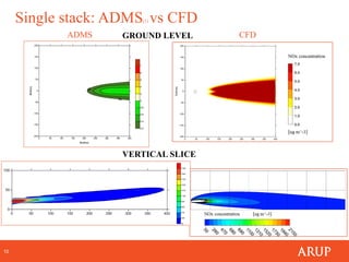
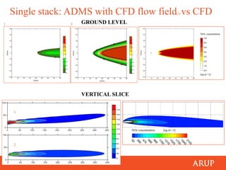
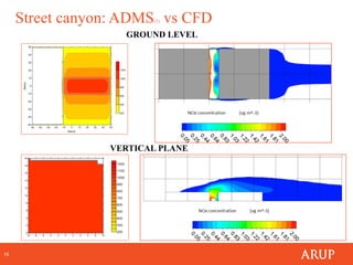
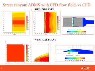
This document compares the Gaussian model and computational fluid dynamics (CFD) for assessing pollutant dispersion, specifically in complex urban environments. It presents results from an analysis comparing the American Meteorological Society/Environmental Protection Agency Regulatory Model (ADMS) Gaussian model to a CFD model. For a single stack and road source in flat terrain, ADMS predicted similar or slightly higher concentrations than CFD. However, for a street canyon scenario, CFD performed better by capturing the three-dimensional and unsteady flow, while ADMS had limitations representing the complex geometry. Further development is still needed to improve importing CFD flow fields into ADMS.