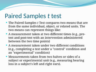
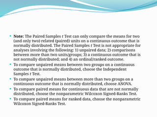
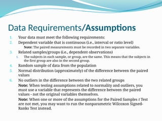
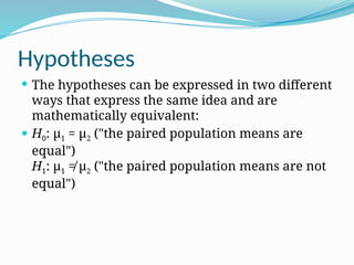
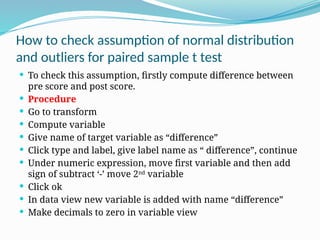
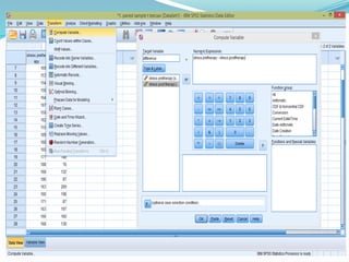
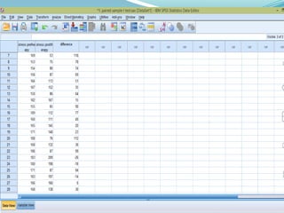
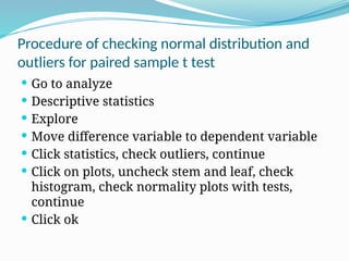
Paired sample t test
By Mrs. Aneeqa Waheed
Paired Samples t test
 The Paired Samples t Test compares two means that are
from the same individual, object, or related units. The
two means can represent things like:
 A measurement taken at two different times (e.g., pre-
test and post-test with an intervention administered
between the two time points)
 A measurement taken under two different conditions
(e.g., completing a test under a "control" condition and
an "experimental" condition)
 Measurements taken from two halves or sides of a
subject or experimental unit (e.g., measuring hearing
loss in a subject's left and right ears).
Purpose
 The purpose of the test is to determine whether
there is statistical evidence that the mean
difference between paired observations on a
particular outcome is significantly different from
zero. The Paired Samples t Test is a parametric
test.
 This test is also known as:
 Dependent t Test
 Paired t Test
 Repeated Measures t Test
 The variable used in this test is known as:
 Dependent variable, or test variable
(continuous), measured at two different times or
for two related conditions or units
Uses of paired sample t test
 The Paired Samples t Test is commonly used to
test the following:
 Statistical difference between two time points
 Statistical difference between two conditions
 Statistical difference between two measurements
 Statistical difference between a matched pair
 Note: The Paired Samples t Test can only compare the means for two
(and only two) related (paired) units on a continuous outcome that is
normally distributed. The Paired Samples t Test is not appropriate for
analyses involving the following: 1) unpaired data; 2) comparisons
between more than two units/groups; 3) a continuous outcome that is
not normally distributed; and 4) an ordinal/ranked outcome.
 To compare unpaired means between two groups on a continuous
outcome that is normally distributed, choose the Independent
Samples t Test.
 To compare unpaired means between more than two groups on a
continuous outcome that is normally distributed, choose ANOVA.
 To compare paired means for continuous data that are not normally
distributed, choose the nonparametric Wilcoxon Signed-Ranks Test.
 To compare paired means for ranked data, choose the nonparametric
Wilcoxon Signed-Ranks Test.
Data Requirements/Assumptions
1. Your data must meet the following requirements:
2. Dependent variable that is continuous (i.e., interval or ratio level)
Note: The paired measurements must be recorded in two separate variables.
3. Related samples/groups (i.e., dependent observations)
1. The subjects in each sample, or group, are the same. This means that the subjects in
the first group are also in the second group.
4. Random sample of data from the population
5. Normal distribution (approximately) of the difference between the paired
values
6. No outliers in the difference between the two related groups
Note: When testing assumptions related to normality and outliers, you
must use a variable that represents the difference between the paired
values - not the original variables themselves.
Note: When one or more of the assumptions for the Paired Samples t Test
are not met, you may want to run the nonparametric Wilcoxon Signed-
Ranks Test instead.
Hypotheses
 The hypotheses can be expressed in two different
ways that express the same idea and are
mathematically equivalent:
 H0: µ1 = µ2 ("the paired population means are
equal")
H1: µ1 ≠ µ2 ("the paired population means are not
equal")
Data
How to check assumption of normal distribution
and outliers for paired sample t test
 To check this assumption, firstly compute difference between
pre score and post score.
 Procedure
 Go to transform
 Compute variable
 Give name of target variable as “difference”
 Click type and label, give label name as “ difference”, continue
 Under numeric expression, move first variable and then add
sign of subtract ‘-’ move 2nd
variable
 Click ok
 In data view new variable is added with name “difference”
 Make decimals to zero in variable view
Procedure of checking normal distribution and
outliers for paired sample t test
 Go to analyze
 Descriptive statistics
 Explore
 Move difference variable to dependent variable
 Click statistics, check outliers, continue
 Click on plots, uncheck stem and leaf, check
histogram, check normality plots with tests,
continue
 Click ok
Interpretation of output of normality
 In order for your data to be approximately normally distributed, the value of skewness should be
between -1.00 to +1.00 and the value of kurtosis should be between -2.00 to +2.00
 As a general rule of thumb: If skewness is less than -1 or greater than 1, the
distribution is highly skewed. If skewness is between -1 and -0.5 or between 0.5 and 1,
the distribution is moderately skewed. If skewness is between -0.5 and 0.5, the
distribution is approximately symmetric.
 Another method is, see the skewness and divide the value of statistic by standard error. You will
get z value. This value should be between -1.96 - +1.96
 Another method is to see Shapiro-wilk test. In order for our data to be normal, The sig. value/p
value in Shapiro wilk test should be greater than .05. the value less than .05 means that the
distribution of our variable is significantly different from normal distribution.
 Another approach is to look for histogram… it should be shown as bell shaped curve.. it should
not be positively or negatively skewed.
 Another approach is to see normal Q-Q plot also known as quantile quantile plot.. all the points
should follow the line. If the data is normally distributed, the points in the QQ-normal plot lie
on a straight diagonal line. You can add this line to you QQ plot with the command qqline(x) ,
where x is the vector of values. The deviations from the straight line are minimal. This
indicates normal distribution.
Interpretation of outliers
 An outlier is an observation that lies an
abnormal distance from other values in a
random sample from a population.
 In Output window: Go to Boxplot > Look at
circles and *. These are potential outliers. If
there's none, then there's no potential outliers in
your dataset.
 If there are circles or *, then there are potential
outliers in your dataset.
Procedure of Paired sample t test
 Go to Analyze
 Compare means
 Click on Paired sample t test
 Move 1st variable in variable 1 of pair 1
 Move 2nd
variable in variable 2 of pair 1
 Click ok
Effect size calculator
 According to Cohen (1988)
 0.1 small
 0.3 medium
 0.6 large
Criteria of effect size
Table and interpretation according to APA 7

A statistical test with SPSS steps paired sample t test.pptx

  • 1.
    Paired sample ttest By Mrs. Aneeqa Waheed
  • 2.
    Paired Samples ttest  The Paired Samples t Test compares two means that are from the same individual, object, or related units. The two means can represent things like:  A measurement taken at two different times (e.g., pre- test and post-test with an intervention administered between the two time points)  A measurement taken under two different conditions (e.g., completing a test under a "control" condition and an "experimental" condition)  Measurements taken from two halves or sides of a subject or experimental unit (e.g., measuring hearing loss in a subject's left and right ears).
  • 3.
    Purpose  The purposeof the test is to determine whether there is statistical evidence that the mean difference between paired observations on a particular outcome is significantly different from zero. The Paired Samples t Test is a parametric test.
  • 4.
     This testis also known as:  Dependent t Test  Paired t Test  Repeated Measures t Test  The variable used in this test is known as:  Dependent variable, or test variable (continuous), measured at two different times or for two related conditions or units
  • 5.
    Uses of pairedsample t test  The Paired Samples t Test is commonly used to test the following:  Statistical difference between two time points  Statistical difference between two conditions  Statistical difference between two measurements  Statistical difference between a matched pair
  • 6.
     Note: ThePaired Samples t Test can only compare the means for two (and only two) related (paired) units on a continuous outcome that is normally distributed. The Paired Samples t Test is not appropriate for analyses involving the following: 1) unpaired data; 2) comparisons between more than two units/groups; 3) a continuous outcome that is not normally distributed; and 4) an ordinal/ranked outcome.  To compare unpaired means between two groups on a continuous outcome that is normally distributed, choose the Independent Samples t Test.  To compare unpaired means between more than two groups on a continuous outcome that is normally distributed, choose ANOVA.  To compare paired means for continuous data that are not normally distributed, choose the nonparametric Wilcoxon Signed-Ranks Test.  To compare paired means for ranked data, choose the nonparametric Wilcoxon Signed-Ranks Test.
  • 7.
    Data Requirements/Assumptions 1. Yourdata must meet the following requirements: 2. Dependent variable that is continuous (i.e., interval or ratio level) Note: The paired measurements must be recorded in two separate variables. 3. Related samples/groups (i.e., dependent observations) 1. The subjects in each sample, or group, are the same. This means that the subjects in the first group are also in the second group. 4. Random sample of data from the population 5. Normal distribution (approximately) of the difference between the paired values 6. No outliers in the difference between the two related groups Note: When testing assumptions related to normality and outliers, you must use a variable that represents the difference between the paired values - not the original variables themselves. Note: When one or more of the assumptions for the Paired Samples t Test are not met, you may want to run the nonparametric Wilcoxon Signed- Ranks Test instead.
  • 8.
    Hypotheses  The hypothesescan be expressed in two different ways that express the same idea and are mathematically equivalent:  H0: µ1 = µ2 ("the paired population means are equal") H1: µ1 ≠ µ2 ("the paired population means are not equal")
  • 9.
  • 10.
    How to checkassumption of normal distribution and outliers for paired sample t test  To check this assumption, firstly compute difference between pre score and post score.  Procedure  Go to transform  Compute variable  Give name of target variable as “difference”  Click type and label, give label name as “ difference”, continue  Under numeric expression, move first variable and then add sign of subtract ‘-’ move 2nd variable  Click ok  In data view new variable is added with name “difference”  Make decimals to zero in variable view
  • 13.
    Procedure of checkingnormal distribution and outliers for paired sample t test  Go to analyze  Descriptive statistics  Explore  Move difference variable to dependent variable  Click statistics, check outliers, continue  Click on plots, uncheck stem and leaf, check histogram, check normality plots with tests, continue  Click ok
  • 17.
    Interpretation of outputof normality  In order for your data to be approximately normally distributed, the value of skewness should be between -1.00 to +1.00 and the value of kurtosis should be between -2.00 to +2.00  As a general rule of thumb: If skewness is less than -1 or greater than 1, the distribution is highly skewed. If skewness is between -1 and -0.5 or between 0.5 and 1, the distribution is moderately skewed. If skewness is between -0.5 and 0.5, the distribution is approximately symmetric.  Another method is, see the skewness and divide the value of statistic by standard error. You will get z value. This value should be between -1.96 - +1.96  Another method is to see Shapiro-wilk test. In order for our data to be normal, The sig. value/p value in Shapiro wilk test should be greater than .05. the value less than .05 means that the distribution of our variable is significantly different from normal distribution.  Another approach is to look for histogram… it should be shown as bell shaped curve.. it should not be positively or negatively skewed.  Another approach is to see normal Q-Q plot also known as quantile quantile plot.. all the points should follow the line. If the data is normally distributed, the points in the QQ-normal plot lie on a straight diagonal line. You can add this line to you QQ plot with the command qqline(x) , where x is the vector of values. The deviations from the straight line are minimal. This indicates normal distribution.
  • 18.
    Interpretation of outliers An outlier is an observation that lies an abnormal distance from other values in a random sample from a population.  In Output window: Go to Boxplot > Look at circles and *. These are potential outliers. If there's none, then there's no potential outliers in your dataset.  If there are circles or *, then there are potential outliers in your dataset.
  • 19.
    Procedure of Pairedsample t test  Go to Analyze  Compare means  Click on Paired sample t test  Move 1st variable in variable 1 of pair 1  Move 2nd variable in variable 2 of pair 1  Click ok
  • 21.
  • 22.
     According toCohen (1988)  0.1 small  0.3 medium  0.6 large Criteria of effect size
  • 23.
    Table and interpretationaccording to APA 7