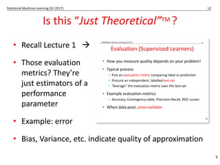
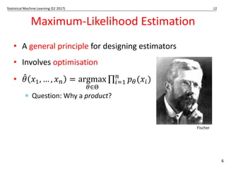
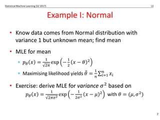
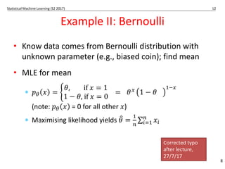
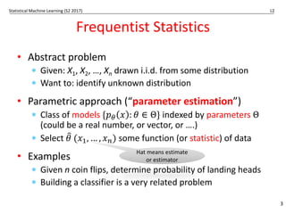
COMP90051 Statistical Machine Learning
Semester 2, 2017
Lecturer: Trevor Cohn
2. Statistical Schools
Adapted from slides by Ben Rubinstein
Statistical Machine Learning (S2 2017) L2
Statistical Schools of Thought
2
Based on Berkeley CS 294-34 tutorial slides by Ariel Kleiner
Remainder of lecture is to provide intuition into how
algorithms in this subject come about and inter-relate
Statistical Machine Learning (S2 2017) L2
Frequentist Statistics
โ€ข Abstract problem
* Given: X1, X2, โ€ฆ, Xn drawn i.i.d. from some distribution
* Want to: identify unknown distribution
โ€ข Parametric approach (โ€œparameter estimationโ€)
* Class of models {๐‘# ๐‘ฅ : ๐œƒ โˆˆ ฮ˜} indexed by parameters ฮ˜
(could be a real number, or vector, or โ€ฆ.)
* Select ๐œƒ
* (๐‘ฅ-, โ€ฆ , ๐‘ฅ0) some function (or statistic) of data
โ€ข Examples
* Given n coin flips, determine probability of landing heads
* Building a classifier is a very related problem
3
Hat means estimate
or estimator
Statistical Machine Learning (S2 2017) L2
How do Frequentists Evaluate Estimators?
โ€ข Bias: ๐ต# ๐œƒ
3 = ๐ธ# ๐œƒ
3 ๐‘‹-, โ€ฆ , ๐‘‹0 โˆ’ ๐œƒ
โ€ข Variance: ๐‘‰๐‘Ž๐‘Ÿ# ๐œƒ
3 = ๐ธ# (๐œƒ
3 โˆ’ ๐ธ#[๐œƒ
3])=
* Efficiency: estimate has minimal variance
โ€ข Square loss vs bias-variance
๐ธ# ๐œƒ โˆ’ ๐œƒ
3 =
= [๐ต(๐œƒ)]=
+๐‘‰๐‘Ž๐‘Ÿ#(๐œƒ
3)
โ€ข Consistency: ๐œƒ
3 ๐‘‹-, โ€ฆ , ๐‘‹0 converges to ๐œƒ as n gets
big
โ€ฆ more on this later in the subject โ€ฆ
4
Subscript q
means data really
comes from pq
๐œƒ
* still function of
data
Statistical Machine Learning (S2 2017) L2
Is this โ€œJust Theoreticalโ€TM ?
โ€ข Recall Lecture 1 ร 
โ€ข Those evaluation
metrics? Theyโ€™re
just estimators of a
performance
parameter
โ€ข Example: error
โ€ข Bias, Variance, etc. indicate quality of approximation
5
COMP90051 Machine Learning (S2 2017) L1
Evaluation (Supervised Learners)
โ€ข How you measure quality depends on your problem!
โ€ข Typical process
* Pick an evaluation metric comparing label vs prediction
* Procure an independent, labelled test set
* โ€œAverageโ€ the evaluation metric over the test set
โ€ข Example evaluation metrics
* Accuracy, Contingency table, Precision-Recall, ROC curves
โ€ข When data poor, cross-validate
22
Statistical Machine Learning (S2 2017) L2
Maximum-Likelihood Estimation
โ€ข A general principle for designing estimators
โ€ข Involves optimisation
โ€ข ๐œƒ
3 ๐‘ฅ-, โ€ฆ , ๐‘ฅ0 = argmax
#โˆˆD
โˆ ๐‘#(๐‘ฅF)
0
FG-
* Question: Why a product?
6
Fischer
Statistical Machine Learning (S2 2017) L2
Example I: Normal
โ€ข Know data comes from Normal distribution with
variance 1 but unknown mean; find mean
โ€ข MLE for mean
* ๐‘# ๐‘ฅ =
-
=H
exp โˆ’
-
=
๐‘ฅ โˆ’ ๐œƒ =
* Maximising likelihood yields ๐œƒ
* =
-
0
โˆ‘ ๐‘ฅF
0
FG-
โ€ข Exercise: derive MLE for variance ๐œŽ=
based on
๐‘# ๐‘ฅ =
-
=HNO
exp โˆ’
-
=NO ๐‘ฅ โˆ’ ๐œ‡ = with ๐œƒ = (๐œ‡, ๐œŽ=)
7
Statistical Machine Learning (S2 2017) L2
Example II: Bernoulli
โ€ข Know data comes from Bernoulli distribution with
unknown parameter (e.g., biased coin); find mean
โ€ข MLE for mean
* ๐‘# ๐‘ฅ = Q
๐œƒ, if ๐‘ฅ = 1
1 โˆ’ ๐œƒ, if ๐‘ฅ = 0
= ๐œƒV 1 โˆ’ ๐œƒ
-WV
(note: ๐‘# ๐‘ฅ = 0 for all other ๐‘ฅ)
* Maximising likelihood yields ๐œƒ
* =
-
0
โˆ‘ ๐‘ฅF
0
FG-
8
Corrected typo
after lecture,
27/7/17
Statistical Machine Learning (S2 2017) L2
MLE โ€˜algorithmโ€™
1. given data ๐‘ฅ-, โ€ฆ , ๐‘ฅ0 define probability distribution,
๐‘#, assumed to have generated the data
2. express likelihood of data, โˆ ๐‘#(๐‘ฅF)
0
FG-
(usually its logarithmโ€ฆ why?)
3. optimise to find best (most likely) parameters ๐œƒ
3
1. take partial derivatives of log likelihood wrt ๐œƒ
2. set to 0 and solve
(failing that, use iterative gradient method)
9
Statistical Machine Learning (S2 2017) L2
Bayesian Statistics
โ€ข Probabilities correspond to beliefs
โ€ข Parameters
* Modeled as r.v.โ€™s having distributions
* Prior belief in ๐œƒ encoded by prior distribution P(๐œƒ)
* Write likelihood of data P(๐‘‹) as conditional P(X|๐œƒ)
* Rather than point estimate ๐œƒ
*, Bayesians update belief P(๐œƒ)
with observed data to P(๐œƒ|๐‘‹) the posterior distribution
10
Laplace
Statistical Machine Learning (S2 2017) L2
More Detail (Probabilistic Inference)
โ€ข Bayesian machine learning
* Start with prior P(๐œƒ) and likelihood P(๐‘‹|๐œƒ)
* Observe data ๐‘‹ = ๐‘ฅ
* Update prior to posterior P(๐œƒ|๐‘‹ = ๐‘ฅ)
โ€ข Weโ€™ll later cover tools to get the posterior
* Bayes Theorem: reverses order of conditioning
๐‘ƒ ๐œƒ ๐‘‹ = ๐‘ฅ =
๐‘ƒ ๐‘‹ = ๐‘ฅ ๐œƒ ๐‘ƒ(๐œƒ)
๐‘ƒ(๐‘‹ = ๐‘ฅ)
* Marginalisation: eliminates unwanted variables
P ๐‘‹ = ๐‘ฅ =  ๐‘ƒ(๐‘‹ = ๐‘ฅ, ๐œƒ = ๐‘ก)
^
11
Bayes
Statistical Machine Learning (S2 2017) L2
Example
โ€ข We model ๐‘‹|๐œƒ as ๐‘(๐œƒ, 1) with prior N(0,1)
โ€ข Suppose we observe X=1, then update posterior
๐‘ƒ ๐œƒ ๐‘‹ = 1 =
` ๐‘‹ = 1 ๐œƒ `(#)
`(aG-)
โˆ ๐‘ƒ ๐‘‹ = 1 ๐œƒ ๐‘ƒ ๐œƒ
=
-
=H
๐‘’๐‘ฅ๐‘ โˆ’
(-W#)O
=
-
=H
๐‘’๐‘ฅ๐‘ โˆ’
#O
=
โˆ ๐‘ 0.5,0.5
NB: allowed to push constants out front and โ€œignoreโ€ as
these get taken care of by normalisation
12
Statistical Machine Learning (S2 2017) L2
How Bayesians Make Point Estimates
โ€ข They donโ€™t, unless forced at gunpoint!
* The posterior carries full information, why discard it?
โ€ข But, there are common approaches
* Posterior mean ๐ธ#|a ๐œƒ = โˆซ ๐œƒ๐‘ƒ ๐œƒ ๐‘‹ ๐‘‘๐œƒ
* Posterior mode argmax
#
๐‘ƒ(๐œƒ|๐‘‹) (max a posteriori or MAP)
13
๐‘ƒ(๐œƒ|๐‘‹)
๐œƒ
๐œƒMAP
Statistical Machine Learning (S2 2017) L2
MLE in Bayesian context
โ€ข MLE formulation: find parameters that best fit data
๐œƒ
3 = argmax# ๐‘ƒ ๐‘‹ = ๐‘ฅ ๐œƒ
โ€ข Consider the MAP under a Bayesian formulation
๐œƒ
3 = ๐‘ƒ ๐œƒ ๐‘‹ = ๐‘ฅ
= argmax#
๐‘ƒ ๐‘‹ = ๐‘ฅ ๐œƒ ๐‘ƒ ๐œƒ
๐‘ƒ ๐‘‹ = ๐‘ฅ
= argmax# ๐‘ƒ ๐‘‹ = ๐‘ฅ ๐œƒ ๐‘ƒ ๐œƒ
โ€ข Difference is prior ๐‘ƒ ๐œƒ ; assumed uniform for MLE
14
Statistical Machine Learning (S2 2017) L2
Parametric vs Non-Parametric Models
Parametric Non-Parametric
Determined by fixed, finite
number of parameters
Number of parameters grows
with data, potentially infinite
Limited flexibility More flexible
Efficient statistically and
computationally
Less efficient
15
Examples to come! There are non/parametric models
in both the frequentist and Bayesian schools.
Statistical Machine Learning (S2 2017) L2
Generative vs. Discriminative Models
โ€ข Xโ€™s are instances, Yโ€™s are labels (supervised setting!)
* Given: i.i.d. data (X1, Y1),โ€ฆ ,(Xn, Yn)
* Find model that can predict Y of new X
โ€ข Generative approach
* Model full joint P(X, Y)
โ€ข Discriminative approach
* Model conditional P(Y|X) only
โ€ข Both have proโ€™s and conโ€™s
16
Examples to come! There are generative/discriminative
models in both the frequentist and Bayesian schools.
Statistical Machine Learning (S2 2017) L2
Summary
โ€ข Philosophies: frequentist vs. Bayesian
โ€ข Principles behind many learners:
* MLE
* Probabilistic inference, MAP
โ€ข Discriminative vs. Generative models
17

A presentation about machine learning and NN

  • 1.
    COMP90051 Statistical MachineLearning Semester 2, 2017 Lecturer: Trevor Cohn 2. Statistical Schools Adapted from slides by Ben Rubinstein
  • 2.
    Statistical Machine Learning(S2 2017) L2 Statistical Schools of Thought 2 Based on Berkeley CS 294-34 tutorial slides by Ariel Kleiner Remainder of lecture is to provide intuition into how algorithms in this subject come about and inter-relate
  • 3.
    Statistical Machine Learning(S2 2017) L2 Frequentist Statistics โ€ข Abstract problem * Given: X1, X2, โ€ฆ, Xn drawn i.i.d. from some distribution * Want to: identify unknown distribution โ€ข Parametric approach (โ€œparameter estimationโ€) * Class of models {๐‘# ๐‘ฅ : ๐œƒ โˆˆ ฮ˜} indexed by parameters ฮ˜ (could be a real number, or vector, or โ€ฆ.) * Select ๐œƒ * (๐‘ฅ-, โ€ฆ , ๐‘ฅ0) some function (or statistic) of data โ€ข Examples * Given n coin flips, determine probability of landing heads * Building a classifier is a very related problem 3 Hat means estimate or estimator
  • 4.
    Statistical Machine Learning(S2 2017) L2 How do Frequentists Evaluate Estimators? โ€ข Bias: ๐ต# ๐œƒ 3 = ๐ธ# ๐œƒ 3 ๐‘‹-, โ€ฆ , ๐‘‹0 โˆ’ ๐œƒ โ€ข Variance: ๐‘‰๐‘Ž๐‘Ÿ# ๐œƒ 3 = ๐ธ# (๐œƒ 3 โˆ’ ๐ธ#[๐œƒ 3])= * Efficiency: estimate has minimal variance โ€ข Square loss vs bias-variance ๐ธ# ๐œƒ โˆ’ ๐œƒ 3 = = [๐ต(๐œƒ)]= +๐‘‰๐‘Ž๐‘Ÿ#(๐œƒ 3) โ€ข Consistency: ๐œƒ 3 ๐‘‹-, โ€ฆ , ๐‘‹0 converges to ๐œƒ as n gets big โ€ฆ more on this later in the subject โ€ฆ 4 Subscript q means data really comes from pq ๐œƒ * still function of data
  • 5.
    Statistical Machine Learning(S2 2017) L2 Is this โ€œJust Theoreticalโ€TM ? โ€ข Recall Lecture 1 ร  โ€ข Those evaluation metrics? Theyโ€™re just estimators of a performance parameter โ€ข Example: error โ€ข Bias, Variance, etc. indicate quality of approximation 5 COMP90051 Machine Learning (S2 2017) L1 Evaluation (Supervised Learners) โ€ข How you measure quality depends on your problem! โ€ข Typical process * Pick an evaluation metric comparing label vs prediction * Procure an independent, labelled test set * โ€œAverageโ€ the evaluation metric over the test set โ€ข Example evaluation metrics * Accuracy, Contingency table, Precision-Recall, ROC curves โ€ข When data poor, cross-validate 22
  • 6.
    Statistical Machine Learning(S2 2017) L2 Maximum-Likelihood Estimation โ€ข A general principle for designing estimators โ€ข Involves optimisation โ€ข ๐œƒ 3 ๐‘ฅ-, โ€ฆ , ๐‘ฅ0 = argmax #โˆˆD โˆ ๐‘#(๐‘ฅF) 0 FG- * Question: Why a product? 6 Fischer
  • 7.
    Statistical Machine Learning(S2 2017) L2 Example I: Normal โ€ข Know data comes from Normal distribution with variance 1 but unknown mean; find mean โ€ข MLE for mean * ๐‘# ๐‘ฅ = - =H exp โˆ’ - = ๐‘ฅ โˆ’ ๐œƒ = * Maximising likelihood yields ๐œƒ * = - 0 โˆ‘ ๐‘ฅF 0 FG- โ€ข Exercise: derive MLE for variance ๐œŽ= based on ๐‘# ๐‘ฅ = - =HNO exp โˆ’ - =NO ๐‘ฅ โˆ’ ๐œ‡ = with ๐œƒ = (๐œ‡, ๐œŽ=) 7
  • 8.
    Statistical Machine Learning(S2 2017) L2 Example II: Bernoulli โ€ข Know data comes from Bernoulli distribution with unknown parameter (e.g., biased coin); find mean โ€ข MLE for mean * ๐‘# ๐‘ฅ = Q ๐œƒ, if ๐‘ฅ = 1 1 โˆ’ ๐œƒ, if ๐‘ฅ = 0 = ๐œƒV 1 โˆ’ ๐œƒ -WV (note: ๐‘# ๐‘ฅ = 0 for all other ๐‘ฅ) * Maximising likelihood yields ๐œƒ * = - 0 โˆ‘ ๐‘ฅF 0 FG- 8 Corrected typo after lecture, 27/7/17
  • 9.
    Statistical Machine Learning(S2 2017) L2 MLE โ€˜algorithmโ€™ 1. given data ๐‘ฅ-, โ€ฆ , ๐‘ฅ0 define probability distribution, ๐‘#, assumed to have generated the data 2. express likelihood of data, โˆ ๐‘#(๐‘ฅF) 0 FG- (usually its logarithmโ€ฆ why?) 3. optimise to find best (most likely) parameters ๐œƒ 3 1. take partial derivatives of log likelihood wrt ๐œƒ 2. set to 0 and solve (failing that, use iterative gradient method) 9
  • 10.
    Statistical Machine Learning(S2 2017) L2 Bayesian Statistics โ€ข Probabilities correspond to beliefs โ€ข Parameters * Modeled as r.v.โ€™s having distributions * Prior belief in ๐œƒ encoded by prior distribution P(๐œƒ) * Write likelihood of data P(๐‘‹) as conditional P(X|๐œƒ) * Rather than point estimate ๐œƒ *, Bayesians update belief P(๐œƒ) with observed data to P(๐œƒ|๐‘‹) the posterior distribution 10 Laplace
  • 11.
    Statistical Machine Learning(S2 2017) L2 More Detail (Probabilistic Inference) โ€ข Bayesian machine learning * Start with prior P(๐œƒ) and likelihood P(๐‘‹|๐œƒ) * Observe data ๐‘‹ = ๐‘ฅ * Update prior to posterior P(๐œƒ|๐‘‹ = ๐‘ฅ) โ€ข Weโ€™ll later cover tools to get the posterior * Bayes Theorem: reverses order of conditioning ๐‘ƒ ๐œƒ ๐‘‹ = ๐‘ฅ = ๐‘ƒ ๐‘‹ = ๐‘ฅ ๐œƒ ๐‘ƒ(๐œƒ) ๐‘ƒ(๐‘‹ = ๐‘ฅ) * Marginalisation: eliminates unwanted variables P ๐‘‹ = ๐‘ฅ = ๐‘ƒ(๐‘‹ = ๐‘ฅ, ๐œƒ = ๐‘ก) ^ 11 Bayes
  • 12.
    Statistical Machine Learning(S2 2017) L2 Example โ€ข We model ๐‘‹|๐œƒ as ๐‘(๐œƒ, 1) with prior N(0,1) โ€ข Suppose we observe X=1, then update posterior ๐‘ƒ ๐œƒ ๐‘‹ = 1 = ` ๐‘‹ = 1 ๐œƒ `(#) `(aG-) โˆ ๐‘ƒ ๐‘‹ = 1 ๐œƒ ๐‘ƒ ๐œƒ = - =H ๐‘’๐‘ฅ๐‘ โˆ’ (-W#)O = - =H ๐‘’๐‘ฅ๐‘ โˆ’ #O = โˆ ๐‘ 0.5,0.5 NB: allowed to push constants out front and โ€œignoreโ€ as these get taken care of by normalisation 12
  • 13.
    Statistical Machine Learning(S2 2017) L2 How Bayesians Make Point Estimates โ€ข They donโ€™t, unless forced at gunpoint! * The posterior carries full information, why discard it? โ€ข But, there are common approaches * Posterior mean ๐ธ#|a ๐œƒ = โˆซ ๐œƒ๐‘ƒ ๐œƒ ๐‘‹ ๐‘‘๐œƒ * Posterior mode argmax # ๐‘ƒ(๐œƒ|๐‘‹) (max a posteriori or MAP) 13 ๐‘ƒ(๐œƒ|๐‘‹) ๐œƒ ๐œƒMAP
  • 14.
    Statistical Machine Learning(S2 2017) L2 MLE in Bayesian context โ€ข MLE formulation: find parameters that best fit data ๐œƒ 3 = argmax# ๐‘ƒ ๐‘‹ = ๐‘ฅ ๐œƒ โ€ข Consider the MAP under a Bayesian formulation ๐œƒ 3 = ๐‘ƒ ๐œƒ ๐‘‹ = ๐‘ฅ = argmax# ๐‘ƒ ๐‘‹ = ๐‘ฅ ๐œƒ ๐‘ƒ ๐œƒ ๐‘ƒ ๐‘‹ = ๐‘ฅ = argmax# ๐‘ƒ ๐‘‹ = ๐‘ฅ ๐œƒ ๐‘ƒ ๐œƒ โ€ข Difference is prior ๐‘ƒ ๐œƒ ; assumed uniform for MLE 14
  • 15.
    Statistical Machine Learning(S2 2017) L2 Parametric vs Non-Parametric Models Parametric Non-Parametric Determined by fixed, finite number of parameters Number of parameters grows with data, potentially infinite Limited flexibility More flexible Efficient statistically and computationally Less efficient 15 Examples to come! There are non/parametric models in both the frequentist and Bayesian schools.
  • 16.
    Statistical Machine Learning(S2 2017) L2 Generative vs. Discriminative Models โ€ข Xโ€™s are instances, Yโ€™s are labels (supervised setting!) * Given: i.i.d. data (X1, Y1),โ€ฆ ,(Xn, Yn) * Find model that can predict Y of new X โ€ข Generative approach * Model full joint P(X, Y) โ€ข Discriminative approach * Model conditional P(Y|X) only โ€ข Both have proโ€™s and conโ€™s 16 Examples to come! There are generative/discriminative models in both the frequentist and Bayesian schools.
  • 17.
    Statistical Machine Learning(S2 2017) L2 Summary โ€ข Philosophies: frequentist vs. Bayesian โ€ข Principles behind many learners: * MLE * Probabilistic inference, MAP โ€ข Discriminative vs. Generative models 17