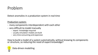
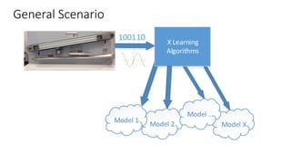
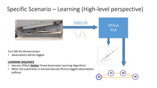
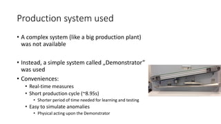
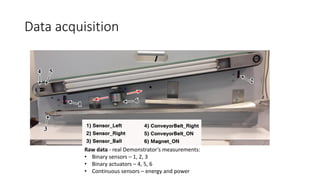
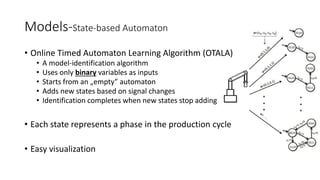
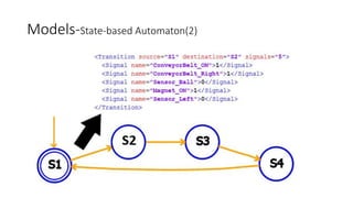
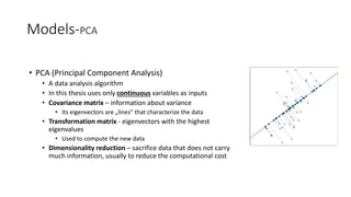
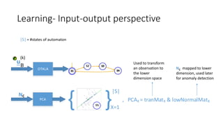
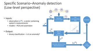
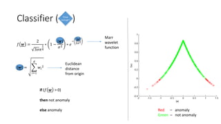
1) The document proposes using machine learning techniques like OTALA and PCA to automatically build models of production systems and detect anomalies in real-time without needing expert knowledge of the system's components. 2) It tests this approach on a "Demonstrator" production system, using OTALA to model normal behavior as a state machine and PCA to reduce data dimensions. It then detects anomalies by comparing new data to these models. 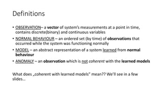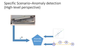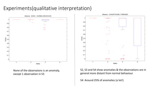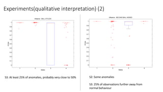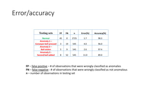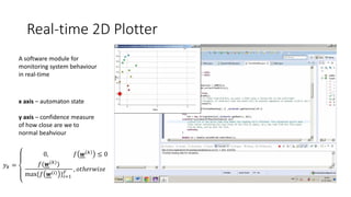3) Experiments show this approach can accurately detect various introduced anomalies, though it cannot diagnose their specific causes. The models also allow monitoring system behavior in real-time.

1. A combined approach for anomaly detection in production systems
using machine learning techniques
Università degli Studi di Trieste
Dipartimento di Ingegneria e Architettura
Corso di Laurea Magistrale in Ingegneria Informatica
Laureando:
David Fanjkutić
Relatore:
prof. Eric Medvet
Correlatori:
dott. Alexander Maier
dott. Andreas Bunte
Anno accademico 2014/2015
Sessione straordinaria

2. Problem
Detect anomalies in a production system in real-time
Production system:
- many components interdependent with each other
- very difficult to model manually
- expert knowledge required
- usually simulation models are built
- very time-consuming and expensive
How to build a model of a system automatically, without knowing its components
or structure, so reducing the need of expert knowledge?
Data-driven modelling

3. Why is it important?
Detect anomalies in RT:
- Fast reaction in production system’s failures
- Big saves in money
Ignore system’s components and structure:
- Independency of the physical components of a system
-> implementable in any production system
(needs only sensor measurements, actuator actions…)

4. Objective
Given measurements:
1. Learn models that represent the production system
2. Use those models for real-time anomaly detection and diagnosisand diagnosis
Anomaly detection – realize that the system is not working properly
Anomaly diagnosis – identify why the system isn’t working properly

5. Production system used
• A complex system (like a big production plant)
was not available
• Instead, a simple system called „Demonstrator”
was used
• Conveniences:
• Real-time measures
• Short production cycle (~8.95s)
• Shorter period of time needed for learning and testing
• Easy to simulate anomalies
• Physical acting upon the Demonstrator

6. Data acquisition
Raw data - real Demonstrator’s measurements:
• Binary sensors – 1, 2, 3
• Binary actuators – 4, 5, 6
• Continuous sensors – energy and power

7. General Scenario
100110
X Learning
Algorithms
Model XModel 2
Model 1
Model …

8. Definitions
• OBSERVATION– a vector of system’s measurements at a point in time,
contains discrete(binary) and continuous variables
• NORMAL BEHAVIOUR – an ordered set (by time) of observations that
occurred while the system was functioning normally
• MODEL – an abstract representation of a system learned from normal
behaviour
• ANOMALY – an observation which is not coherent with the learned models
What does „coherent with learned models” mean?? We’ll see in a few
slides…

9. Models-State-based Automaton
• Online Timed Automaton Learning Algorithm (OTALA)
• A model-identification algorithm
• Uses only binary variables as inputs
• Starts from an „empty” automaton
• Adds new states based on signal changes
• Identification completes when new states stop adding
• Each state represents a phase in the production cycle
• Easy visualization

10. Models-State-based Automaton(2)

11. Models-PCA
• PCA (Principal Component Analysis)
• A data analysis algorithm
• In this thesis uses only continuous variables as inputs
• Covariance matrix – information about variance
• Its eigenvectors are „lines” that characterize the data
• Transformation matrix - eigenvectors with the highest
eigenvalues
• Used to compute the new data
• Dimensionality reduction – sacrifice data that does not carry
much information, usually to reduce the computational cost

12. 100110
OTALA
PCA
Specific Scenario – Learning (High-level perspective)
Turn ON the Demonstrator
• observations will be logged
LEARNING SEQUENCE
• Execute OTALA (Online Timed Automaton Learning Algorithm)
• When the automaton is learned execute PCA on logged observations
(offline)

13. Observations and normal behaviour
( ) is the k-th observation containing only binary variables= 100110
NC = t=𝟏
𝐅
is the continuous normal behaviour, where F is the total number of observations used to represent ituC
(t)
( ) is the k-th observation containing only continuous variables=
uB
(k)
uC
(k)
( , ) is the k-th observationu(k) = 100110
N = t=𝟏
𝐅
𝐮(t) is the normal behaviour, where F is the total number of observations used to represent it

14. Learning- Input-output perspective
|S|= #states of automaton
Used to transform
an observation to
the lower
dimension space
NC mapped to lower
dimension, used later
for anomaly detection
PCA
OTALA
NC
{ }X=1
|S|
, PCAX = tranMatX & lowNormalMatX

15. Specific Scenario–Anomaly detection
(High-level perspective)
Anomaly
detection
u(k)

16. • Inputs:
• observation (u(k)) - a vector containing
system’s measurements
• models – PCA and automaton
• Output:
• binary classification – is it an anomaly?
Specific Scenario–Anomaly detection
(Low-level perspective)
Retrieve
current state
Map to
lower
dimension
Calculate distance from
Normal behaviour
Close
enough?
NO
Anomaly!
u(k)
Get
corresponding
PCA
w(k)
|w(k)
|

17. |𝒘| =
𝑖=1
𝑑
𝑤𝑖
2
Classifier ( )
Euclidean
distance
from origin
Marr
wavelet
function
if (𝑓 𝒘 > 0)
then not anomaly
else anomaly Red – anomaly
Green – not anomaly
Close
enough?
𝑓 𝒘 =
2
3𝜎𝜋
1
4
∗ 1 −
|𝒘|
𝜎2 ∗ 𝑒
−
𝒘
2𝜎2

18. Interpretation of anomalies
• Anomaly – non positive output of the Marr wavelet function
• What does it mean to have 1 anomaly?
• Probably just some noise, wrong measurements…
• Multiple consequent anomalies?
• Probably a real failure

19. Dataset
Training set Testing set
Observations 480 8175
Minutes ~2 ~33
Production
cycles
13 222

20. None of the observaions is an anomaly,
except 1 observation in S3
S2, S3 and S4 show anomalies & the observations are in
general more distant from normal behaviour
S4: Around 25% of anomalies (a lot!)
Experiments(qualitative interpretation)

21. S3: At least 25% of anomalies, probably very close to 50% S2: Some anomalies
S3: 25% of observations further away from
normal behaviour
Experiments(qualitative interpretation) (2)

22. Error/accuracy
Testing sets FP FN n Error(%) Accuracy(%)
Normal 45 0 2725 1.7 98.3
Anomaly 1 –
Conveyor belt pressed 3 19 545 4.0 96.0
Anomaly 2 –
Ball stolen 5 9 545 2.6 97.4
Anomaly 3 -
Second ball added 8 52 545 11.0 89.0
FP – false positive – # of observations that were wrongly classified as anomalies
FN – false negative - # of observations that were wrongly classified as not anomalous
n – number of observations in testing set

23. Real-time 2D Plotter
A software module for
monitoring system behaviour
in real-time
x axis – automaton state
y axis – confidence measure
of how close are we to
normal beahviour
𝑦 𝑘 =
0, 𝑓 𝒘 𝑘 ≤ 0
𝑓(𝒘(𝑘))
max{𝑓 𝒘(𝑖) }𝑖=1
𝐹
, 𝑜𝑡ℎ𝑒𝑟𝑤𝑖𝑠𝑒

24. Conclusion
• The experiments showed that OTALA+PCA can detect anomalies in the
given simple production system
• Advantages:
• independent of the production system
• keeps track in which state the anomaly occurred
(pseudo-diagnosis -> decreases significantly the possible causes of anomalies)
• detects early or late binary sensor change
• Shortcomings:
• cannot diagnose (find cause of) detected anomalies –> eligible for future work

25. La presente tesi è prodotto dello scambio internazionale
presso la Hochschule-Ostwestfalen Lin a Lemgo, Germania
in collaborazione con
Infine
Grazie per l’attenzione