This section discusses secondary ventilation systems used in underground mines. It describes four main types: forcing ventilation, exhausting ventilation, mixed systems, and overlap systems. Forcing ventilation pushes fresh air to the work face while exhausting ventilation extracts contaminated air, drawing in fresh air. The overlap system uses both forcing and exhausting fans placed close to the work face to maximize ventilation effectiveness. The section also outlines factors to consider such as minimum airflow rates to ensure worker safety, dilute exhaust gases, and dilute blasting gases. Prescribed minimum airflow rates vary between regions and are based on work area dimensions, number of workers, engine power, and type of explosives used.


![324 8 Secondary Ventilation
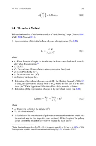
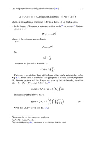
Q(x) = Q f + θ
Po
L
ϒ
1
ϒ + 1
xϒ+1
1
(8.42)
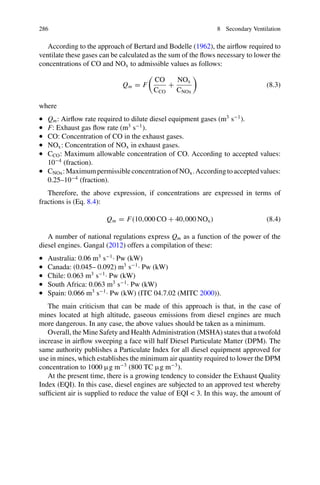
If x = L then Q(x) is the airflow rate at the fan, Qv, we have an equation to calculate
the total leakage along the length of the duct:
Qv = Q f + θ
Po
L
ϒ
1
ϒ + 1
Lϒ+1
1
(8.43a)
And after some simplification we arrive at Eq. 8.43b:
Qv − Q f = θ
Pϒ
o
ϒ + 1
L (8.43b)
Returning to Eq. 8.43a, we can rearrange terms such that:
Qv − Q f
L(ϒ+1)
= θ
1
ϒ + 1
Po
L
ϒ
Which can be substituted in Eq. 8.41, so obtaining Eq. 8.44:
Q(x) = Q f +
Qv − Q f
x
L
Υ +1
(8.44)
Taking the equation for friction losses (Eq. 8.37), at a point, x:
dP(x) = r Q(x)α
dx
then substituting for Q(x) from Eq. 8.44, we obtain Eq. 8.45:
dP(x) = r
Q f +
Qv − Q f
x
L
Υ +1
α
dx (8.45)
Which must be integrated to find the required fan pressure at point x. This can be
done by first doing a Taylor expansion of Eq. 8.45. Taking the first two terms of this
expansion, we have:
dP(x) ≈ r Qα
f
1 +
α
Qv − Q f
Q f
x
L
Υ +1
dx
Which, when integrated for the interval [0, L], with Pf = 0, gives us (Eq. 8.46):
P(x) = r Qα
f
x +
α
Qv − Q f
Q f
1
L
Υ +1
xΥ +2
Υ + 2](https://image.slidesharecdn.com/8secondaryventilation-210412125113/85/8-secondary-ventilation-46-320.jpg)
![8.12 Simplified Solution Following Bertard and Bodelle (1962) 325
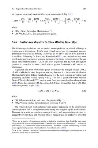
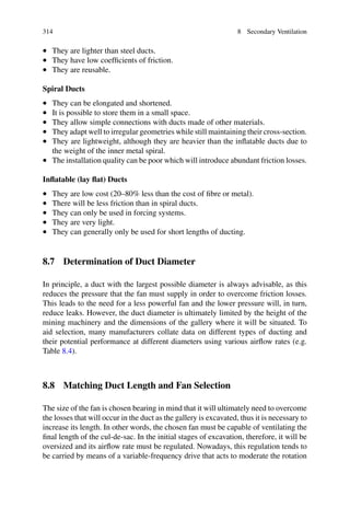
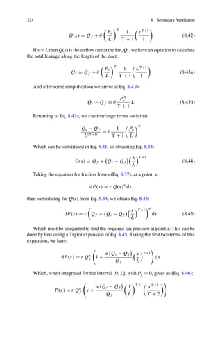
Therefore, the pressure provided by the fan (Pv) is as shown in Eq. 8.46:
Pv = P(x = L) = r Qα
f L
1 +
Qv − Q f
Q f
α
ϒ + 2
(8.46)
Since P0 = r Qα
f L, this simplifies to give Eq. 8.47:
Pv = P0
1 +
α
Υ + 2
Qv − Q f
Q f
(8.47)
A more formal solution to Eq. 8.45, in the case of turbulent conditions, (α = 2),
is obtained if we expand the square:
dP(x) = r
Q2
f + 2 Q f
Qv − Q f
x
L
Υ +1
+
Qv − Q f
2
x
L
2(Υ +1)
dx
Which when integrated for the range [0, L], with Pf = 0 as assumed previously,
gives us Eqs. 8.48 and 8.49, as alternative expressions for the calculation of the fan
pressure:
Pv = r Q2
f L
1 +
2
Υ + 2
Qv − Q f
Q f
+
1
2Υ + 3
Qv − Q f
2
Q2
f
(8.48)
Pv = P0
1 +
2
Υ + 2
Qv − Q f
Q f
+
1
2ϒ + 3
Qv − Q f
2
Q2
f
(8.49)
The leak rate (Qv − Qf ) can be obtained from Eq. 8.43a. When leakage is
high (poor installations), the value of (Qv − Qf )2
becomes important, leading to
discrepancies between results given by these expressions and the simplified ones.
In the above expressions, we usually work with the units proposed by Bertard and
Bodelle (1962):
• r: kμ m−1
.
• Pv: mmwc.
• Qv: m3
s−1
.
• Qf : m3
s−1
.
• L: m.
• α: Coefficient of regimen (2 for rigid ducts, 1.7 for flexible ones).
• Θ: Exponent of the leakage law. Values vary from 0.5 to 1.2 from higher to lower
tightness of the conduction.
Exercise 8.8 For proper ventilation, the required airflow flow rate is 1.7 m3
s−1
at
the face of a cul-de-sac. To this end, a metal duct 400 m long of 0.4 m diameter](https://image.slidesharecdn.com/8secondaryventilation-210412125113/85/8-secondary-ventilation-47-320.jpg)


![8.14 Discrete Solution (Step by Step Method) 339
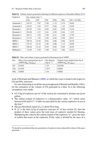
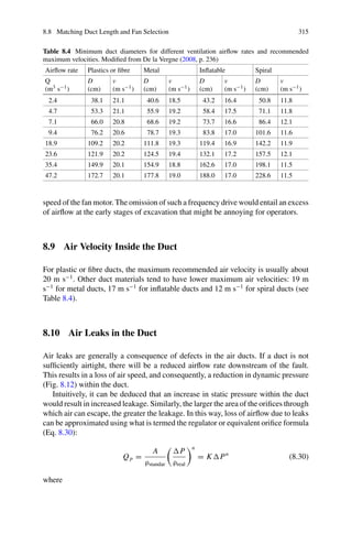
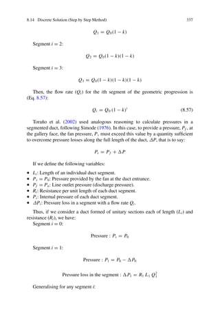
Solution
(a)
The conditions where n = 0 are equivalent to those pertaining to a fan output
without any coupled sections, i.e. in free discharge. It is not possible to use the
derived formula since it is only valid for cases where the fan is connected to a duct
section (n1).
(b)
Here we must use of the propierties of limits, thus, limit of a product of two functions
is equivalent to the product of their limits. In this case, Eq. 8.59, can be expresed
as the product of two limits, first:
lim
k→0
1
(1 − k)2n
= 1
And second:
lim
k→0
(1 − k)2n+2
− (1 − k)2
[(1 − k)2
− 1]
Using the L’Hôpital’s rule for the undeterminate form 0/0, we have:
• Numerator: f
(k) = (−1) (2n + 2) · (1 − k)2n+1
− 2·(1 − k) · (−1)
• Denominator: g
(k) = 2 · (1 − k) · (−1)
Hence:
f
(k)
g(k)
=
2n
2
= n
Therefore:
P = lim
k→0
Ri Li
Q2
f
(1 − k)2n
(1 − k)2n+2
− (1 − k)2
(1 − k)2
− 1
= RLQ2
f · 1 · n
Given that:
nRi Li = RT LT
We have:
P = RT LT Q2
f](https://image.slidesharecdn.com/8secondaryventilation-210412125113/85/8-secondary-ventilation-64-320.jpg)