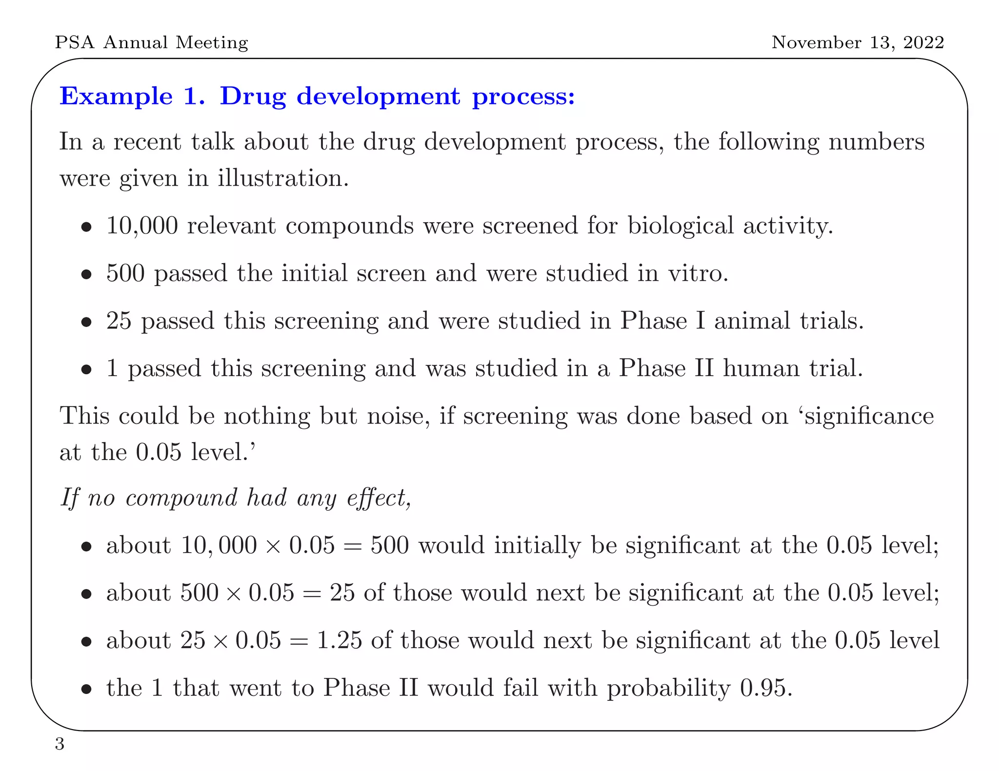
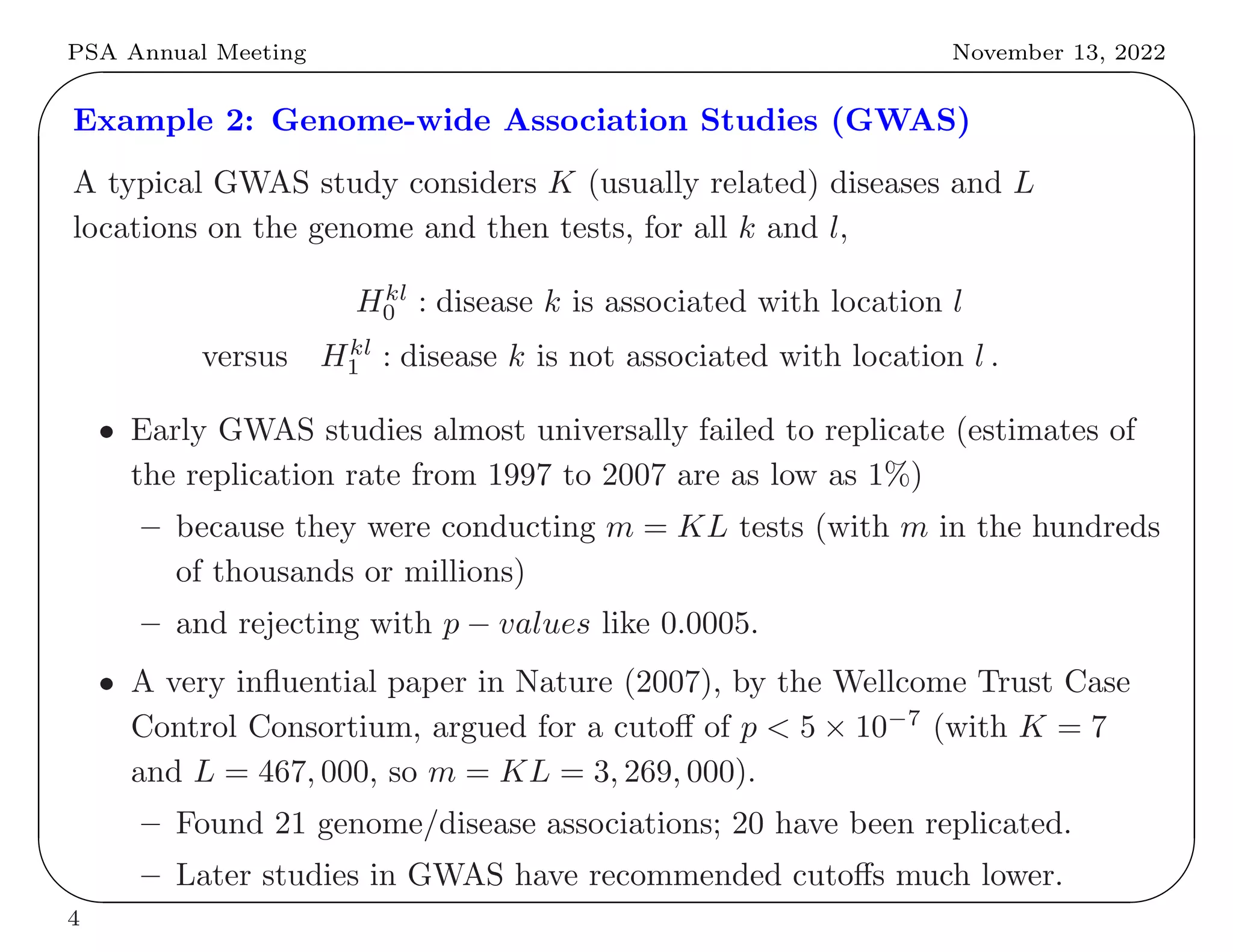
PSA Annual Meeting November 13, 2022
✬
✫
✩
✪
Comparing Frequentist and Bayesian Control
of Multiple Testing
Jim Berger
Duke University
PSA 2022, Pittsburgh, PA
November 13, 2022
1
PSA Annual Meeting November 13, 2022
✬
✫
✩
✪
Outline: four examples
• Drug development process
• Genome-wide association studies, where frequentists and Bayesians both
adjust for multiple testing.
• Optional stopping, where frequentists adjust but Bayesians do not.
• Sequential endpoint testing, where Bayesians adjust but frequentists do
not.
2
PSA Annual Meeting November 13, 2022
✬
✫
✩
✪
Example 1. Drug development process:
In a recent talk about the drug development process, the following numbers
were given in illustration.
• 10,000 relevant compounds were screened for biological activity.
• 500 passed the initial screen and were studied in vitro.
• 25 passed this screening and were studied in Phase I animal trials.
• 1 passed this screening and was studied in a Phase II human trial.
This could be nothing but noise, if screening was done based on ‘significance
at the 0.05 level.’
If no compound had any effect,
• about 10, 000 × 0.05 = 500 would initially be significant at the 0.05 level;
• about 500 × 0.05 = 25 of those would next be significant at the 0.05 level;
• about 25 × 0.05 = 1.25 of those would next be significant at the 0.05 level
• the 1 that went to Phase II would fail with probability 0.95.
3
PSA Annual Meeting November 13, 2022
✬
✫
✩
✪
Example 2: Genome-wide Association Studies (GWAS)
A typical GWAS study considers K (usually related) diseases and L
locations on the genome and then tests, for all k and l,
Hkl
0 : disease k is associated with location l
versus Hkl
1 : disease k is not associated with location l .
• Early GWAS studies almost universally failed to replicate (estimates of
the replication rate from 1997 to 2007 are as low as 1%)
– because they were conducting m = KL tests (with m in the hundreds
of thousands or millions)
– and rejecting with p − values like 0.0005.
• A very influential paper in Nature (2007), by the Wellcome Trust Case
Control Consortium, argued for a cutoff of p < 5 × 10⁻⁷
(with K = 7
and L = 467, 000, so m = KL = 3, 269, 000).
– Found 21 genome/disease associations; 20 have been replicated.
– Later studies in GWAS have recommended cutoffs much lower.
4
PSA Annual Meeting November 13, 2022
✬
✫
✩
✪
Possible corrections for this multiple testing:
• If strong error control is desired (essentially zero incorrect rejections):
– A Frequentist Solution - Bonferonni correction: If one is conducting
m = KL independent tests and wants the probability of any incorrect
rejection to be less than 0.05, then each test should only reject if
p < 0.05/m. (GWAS example: p < 0.05/3, 269, 000 = 1.5 × 10⁻⁸
.)
– A Bayesian solution: Let π1 denote the prior probability of a
disease/gene association, assume that π1 is unknown, and conduct a
Bayesian analysis.
∗ An objective Bayesian might assign π1 a uniform distribution on (0,1).
The posterior distribution of π1 would concentrate on very small values.
∗ A subjective Bayesian would chose the prior distribution to reflect their
beliefs on the plausibility of a disease/gene association.
– It has been observed that both the frequentist and the Bayesian
solution provide strong error control, with the Bayesian solution
having more power in situations of dependent test statistics.
5
PSA Annual Meeting November 13, 2022
✬
✫
✩
✪
• If control of the proportion of true rejections to false rejections is desired.
– A Frequentist Solution - False Discovery Rate
– A Bayesian solution (that chosen in the Nature paper):
∗ They decided that their desired proportion of true rejections to false
rejections is 10:1.
∗ They estimated that the prior odds that a gene is associated with a
disease to not being associated with a disease is
π1
1 − π1
=
1
100, 000
.
∗ They then used Bayes theorem to infer the p − value cutoff.
• Again these tend to give similar answers; how is this when the
approaches seem so different?
6
PSA Annual Meeting November 13, 2022
✬
✫
✩
✪
Example 3. Optional Stopping
The tradition in some sciences is to ignore optional stopping; if one is close
to p = 0.05, go get more data to try get there.
Example: Suppose the null hypothesis (H0) that a normal mean is zero is
true, and tested with a sample of size 100.
• Suppose one obtains p = 0.08.
– Suppose one takes up to four additional samples of size 25,
∗ computing the p-value after each sample, based on the combined data,
and stopping if the new p < 0.05,
∗ and then only reporting p < 0.05 and the combined sample size.
– The chance of obtaining a p < 0.05 with this optional stopping is 2
3
.
– If one repeatedly takes additional samples of size 25, the chance of
obtaining a p < 0.05 is 1.
– Virtually all statisticians and many scientists find this unacceptable and
urge correction for optional stopping when using frequentist tests, as above.
7
PSA Annual Meeting November 13, 2022
✬
✫
✩
✪
• In contrast, a Bayesian analysis does not correct for optional stopping
(the ‘stopping rule’ cancels out in Bayes theorem).
• Suppose one obtains P(H0 | data) = 0.08.
– Suppose one takes up to four additional samples of size 25,
∗ computing P(H0 | data) after each sample, based on the combined
data, and stopping if the new P(H0 | data) < 0.05,
∗ and then just reporting P(H0 | data) < 0.05 and the combined
sample size.
– The chance that P(H0 | data) < 0.05 with this optional stopping is
0.215.
– If one repeatedly takes additional samples of size 25, the chance of
obtaining a P(H0 | data) < 0.05 is 0.22. Futhermore, as one collects
more and more data, P(H0 | data) → 1.
8
PSA Annual Meeting November 13, 2022
✬
✫
✩
✪
Competing intuitions about optional stopping:
Intuition 1. It is wrong to give the investigator multiple tries to prove
something, and not reveal that this was done.
Intuition 2. The data is the data; thoughts the investigator had about the
data shouldn’t change what the data has to say (the stopping rule principal).
Famous example: Two collaborators are monitoring a graduate student
conducting an experiment where the observations are ‘success’ or ‘failure’.
• After 9 successes and 4 failures have been observed, the collaborators
simultaneously tell the graduate student to cease experimenting.
• They separately analyze the data and, to their surprise, one says the data is
‘significant’ (he had planned to stop the experiment after 4 failures) and the
other says it is not (she had planned to take 13 observations).
Intuition here has difficulty; as Savage (1961) said “When I first heard the
stopping rule principle from Barnard in the early 50’s, I thought it was scandalous
that anyone in the profession could espouse a principle so obviously wrong, even as
today I find it scandalous that anyone could deny a principle so obviously right.”
9
PSA Annual Meeting November 13, 2022
✬
✫
✩
✪
Example 4: Sequential endpoint testing. The scenario:
• A sequence of null and alternative hypotheses {H1
0 , H1
1 }, {H2
0 , H2
1 }, . . . ,
that are to be tested sequentially.
– The ordering of the hypotheses is important, and must be
pre-specified.
– Illustration: H1
1 : a new drug provides pain relief, H2
1 : the same drug
reduces blood pressure, and H3
1 : the same drug promotes weight loss.
• The same nominal Type I error, α, is chosen for each hypothesis test.
• The sequential process is as follows:
– Conduct the first test, stopping if H1
0 is not rejected.
– If H1
0 is rejected, perform the second test, stopping or continuing on
depending on whether the second test fails to reject or rejects.
– Continuing on in this fashion, the end result is some sequence
(possibly empty) {H1
0 , H2
0 , . . . , Hm
0 } of rejected null hypotheses, with
m + 1 being the first time one fails to reject.
10
PSA Annual Meeting November 13, 2022
✬
✫
✩
✪
Frequentist Fact:
P(one or more false rejections | H1
ii
, H2
i2
, . . .) ≤ α ,
no matter what sequence of hypotheses is true. Some comments:
• In traditional multiple testing, to obtain an overall level of α for the m
tests, one would need to do the individual tests at (say) nominal level
α/m.
• In sequential endpoint testing, however, not all tests are necessarily
conducted, the crucial reason that no Type I error correction is needed.
Sequential endpoint testing is incompatible with Bayesian reasoning. In
particular, the Bayesian posterior probabilities of the alternative hypotheses
satisfy
P(H1
1 | data) > P(H1
1 , H2
1 | data) > · · · > P(H1
1 , H2
1 , . . . Hm
1 | data) ,
so that increasing numbers of rejections result in less probability being
assigned to all the rejections being correct.
11
PSA Annual Meeting November 13, 2022
✬
✫
✩
✪
Final Thoughts
• Typical multiple testing problems crucially need adjustment, from either
frequentist or Bayesian perspectives,
– although they achieve this from very different directions.
– The Bayesian approach is guaranteed to be fully powered, even with
dependent test statistics.
∗ Indeed, the multiplicity adjustment through prior probabilities is
completely separate from the distributions being tested.
• Optional stopping is contentious, because frequentists adjust and
Bayesians do not.
– They are both right, within their own paradigms.
– It is an advantage of the Bayesian approach that, if the analysis is
indeed Bayesian, it is immune to undisclosed optional stopping.
• Frequentist sequential endpoint testing seems very wrong to me.
12

Comparing Frequentists and Bayesian Control of Multiple Testing

  • 1.
    PSA Annual MeetingNovember 13, 2022 ✬ ✫ ✩ ✪ Comparing Frequentist and Bayesian Control of Multiple Testing Jim Berger Duke University PSA 2022, Pittsburgh, PA November 13, 2022 1
  • 2.
    PSA Annual MeetingNovember 13, 2022 ✬ ✫ ✩ ✪ Outline: four examples • Drug development process • Genome-wide association studies, where frequentists and Bayesians both adjust for multiple testing. • Optional stopping, where frequentists adjust but Bayesians do not. • Sequential endpoint testing, where Bayesians adjust but frequentists do not. 2
  • 3.
    PSA Annual MeetingNovember 13, 2022 ✬ ✫ ✩ ✪ Example 1. Drug development process: In a recent talk about the drug development process, the following numbers were given in illustration. • 10,000 relevant compounds were screened for biological activity. • 500 passed the initial screen and were studied in vitro. • 25 passed this screening and were studied in Phase I animal trials. • 1 passed this screening and was studied in a Phase II human trial. This could be nothing but noise, if screening was done based on ‘significance at the 0.05 level.’ If no compound had any effect, • about 10, 000 × 0.05 = 500 would initially be significant at the 0.05 level; • about 500 × 0.05 = 25 of those would next be significant at the 0.05 level; • about 25 × 0.05 = 1.25 of those would next be significant at the 0.05 level • the 1 that went to Phase II would fail with probability 0.95. 3
  • 4.
    PSA Annual MeetingNovember 13, 2022 ✬ ✫ ✩ ✪ Example 2: Genome-wide Association Studies (GWAS) A typical GWAS study considers K (usually related) diseases and L locations on the genome and then tests, for all k and l, Hkl 0 : disease k is associated with location l versus Hkl 1 : disease k is not associated with location l . • Early GWAS studies almost universally failed to replicate (estimates of the replication rate from 1997 to 2007 are as low as 1%) – because they were conducting m = KL tests (with m in the hundreds of thousands or millions) – and rejecting with p − values like 0.0005. • A very influential paper in Nature (2007), by the Wellcome Trust Case Control Consortium, argued for a cutoff of p < 5 × 10⁻⁷ (with K = 7 and L = 467, 000, so m = KL = 3, 269, 000). – Found 21 genome/disease associations; 20 have been replicated. – Later studies in GWAS have recommended cutoffs much lower. 4
  • 5.
    PSA Annual MeetingNovember 13, 2022 ✬ ✫ ✩ ✪ Possible corrections for this multiple testing: • If strong error control is desired (essentially zero incorrect rejections): – A Frequentist Solution - Bonferonni correction: If one is conducting m = KL independent tests and wants the probability of any incorrect rejection to be less than 0.05, then each test should only reject if p < 0.05/m. (GWAS example: p < 0.05/3, 269, 000 = 1.5 × 10⁻⁸ .) – A Bayesian solution: Let π1 denote the prior probability of a disease/gene association, assume that π1 is unknown, and conduct a Bayesian analysis. ∗ An objective Bayesian might assign π1 a uniform distribution on (0,1). The posterior distribution of π1 would concentrate on very small values. ∗ A subjective Bayesian would chose the prior distribution to reflect their beliefs on the plausibility of a disease/gene association. – It has been observed that both the frequentist and the Bayesian solution provide strong error control, with the Bayesian solution having more power in situations of dependent test statistics. 5
  • 6.
    PSA Annual MeetingNovember 13, 2022 ✬ ✫ ✩ ✪ • If control of the proportion of true rejections to false rejections is desired. – A Frequentist Solution - False Discovery Rate – A Bayesian solution (that chosen in the Nature paper): ∗ They decided that their desired proportion of true rejections to false rejections is 10:1. ∗ They estimated that the prior odds that a gene is associated with a disease to not being associated with a disease is π1 1 − π1 = 1 100, 000 . ∗ They then used Bayes theorem to infer the p − value cutoff. • Again these tend to give similar answers; how is this when the approaches seem so different? 6
  • 7.
    PSA Annual MeetingNovember 13, 2022 ✬ ✫ ✩ ✪ Example 3. Optional Stopping The tradition in some sciences is to ignore optional stopping; if one is close to p = 0.05, go get more data to try get there. Example: Suppose the null hypothesis (H0) that a normal mean is zero is true, and tested with a sample of size 100. • Suppose one obtains p = 0.08. – Suppose one takes up to four additional samples of size 25, ∗ computing the p-value after each sample, based on the combined data, and stopping if the new p < 0.05, ∗ and then only reporting p < 0.05 and the combined sample size. – The chance of obtaining a p < 0.05 with this optional stopping is 2 3 . – If one repeatedly takes additional samples of size 25, the chance of obtaining a p < 0.05 is 1. – Virtually all statisticians and many scientists find this unacceptable and urge correction for optional stopping when using frequentist tests, as above. 7
  • 8.
    PSA Annual MeetingNovember 13, 2022 ✬ ✫ ✩ ✪ • In contrast, a Bayesian analysis does not correct for optional stopping (the ‘stopping rule’ cancels out in Bayes theorem). • Suppose one obtains P(H0 | data) = 0.08. – Suppose one takes up to four additional samples of size 25, ∗ computing P(H0 | data) after each sample, based on the combined data, and stopping if the new P(H0 | data) < 0.05, ∗ and then just reporting P(H0 | data) < 0.05 and the combined sample size. – The chance that P(H0 | data) < 0.05 with this optional stopping is 0.215. – If one repeatedly takes additional samples of size 25, the chance of obtaining a P(H0 | data) < 0.05 is 0.22. Futhermore, as one collects more and more data, P(H0 | data) → 1. 8
  • 9.
    PSA Annual MeetingNovember 13, 2022 ✬ ✫ ✩ ✪ Competing intuitions about optional stopping: Intuition 1. It is wrong to give the investigator multiple tries to prove something, and not reveal that this was done. Intuition 2. The data is the data; thoughts the investigator had about the data shouldn’t change what the data has to say (the stopping rule principal). Famous example: Two collaborators are monitoring a graduate student conducting an experiment where the observations are ‘success’ or ‘failure’. • After 9 successes and 4 failures have been observed, the collaborators simultaneously tell the graduate student to cease experimenting. • They separately analyze the data and, to their surprise, one says the data is ‘significant’ (he had planned to stop the experiment after 4 failures) and the other says it is not (she had planned to take 13 observations). Intuition here has difficulty; as Savage (1961) said “When I first heard the stopping rule principle from Barnard in the early 50’s, I thought it was scandalous that anyone in the profession could espouse a principle so obviously wrong, even as today I find it scandalous that anyone could deny a principle so obviously right.” 9
  • 10.
    PSA Annual MeetingNovember 13, 2022 ✬ ✫ ✩ ✪ Example 4: Sequential endpoint testing. The scenario: • A sequence of null and alternative hypotheses {H1 0 , H1 1 }, {H2 0 , H2 1 }, . . . , that are to be tested sequentially. – The ordering of the hypotheses is important, and must be pre-specified. – Illustration: H1 1 : a new drug provides pain relief, H2 1 : the same drug reduces blood pressure, and H3 1 : the same drug promotes weight loss. • The same nominal Type I error, α, is chosen for each hypothesis test. • The sequential process is as follows: – Conduct the first test, stopping if H1 0 is not rejected. – If H1 0 is rejected, perform the second test, stopping or continuing on depending on whether the second test fails to reject or rejects. – Continuing on in this fashion, the end result is some sequence (possibly empty) {H1 0 , H2 0 , . . . , Hm 0 } of rejected null hypotheses, with m + 1 being the first time one fails to reject. 10
  • 11.
    PSA Annual MeetingNovember 13, 2022 ✬ ✫ ✩ ✪ Frequentist Fact: P(one or more false rejections | H1 ii , H2 i2 , . . .) ≤ α , no matter what sequence of hypotheses is true. Some comments: • In traditional multiple testing, to obtain an overall level of α for the m tests, one would need to do the individual tests at (say) nominal level α/m. • In sequential endpoint testing, however, not all tests are necessarily conducted, the crucial reason that no Type I error correction is needed. Sequential endpoint testing is incompatible with Bayesian reasoning. In particular, the Bayesian posterior probabilities of the alternative hypotheses satisfy P(H1 1 | data) > P(H1 1 , H2 1 | data) > · · · > P(H1 1 , H2 1 , . . . Hm 1 | data) , so that increasing numbers of rejections result in less probability being assigned to all the rejections being correct. 11
  • 12.
    PSA Annual MeetingNovember 13, 2022 ✬ ✫ ✩ ✪ Final Thoughts • Typical multiple testing problems crucially need adjustment, from either frequentist or Bayesian perspectives, – although they achieve this from very different directions. – The Bayesian approach is guaranteed to be fully powered, even with dependent test statistics. ∗ Indeed, the multiplicity adjustment through prior probabilities is completely separate from the distributions being tested. • Optional stopping is contentious, because frequentists adjust and Bayesians do not. – They are both right, within their own paradigms. – It is an advantage of the Bayesian approach that, if the analysis is indeed Bayesian, it is immune to undisclosed optional stopping. • Frequentist sequential endpoint testing seems very wrong to me. 12