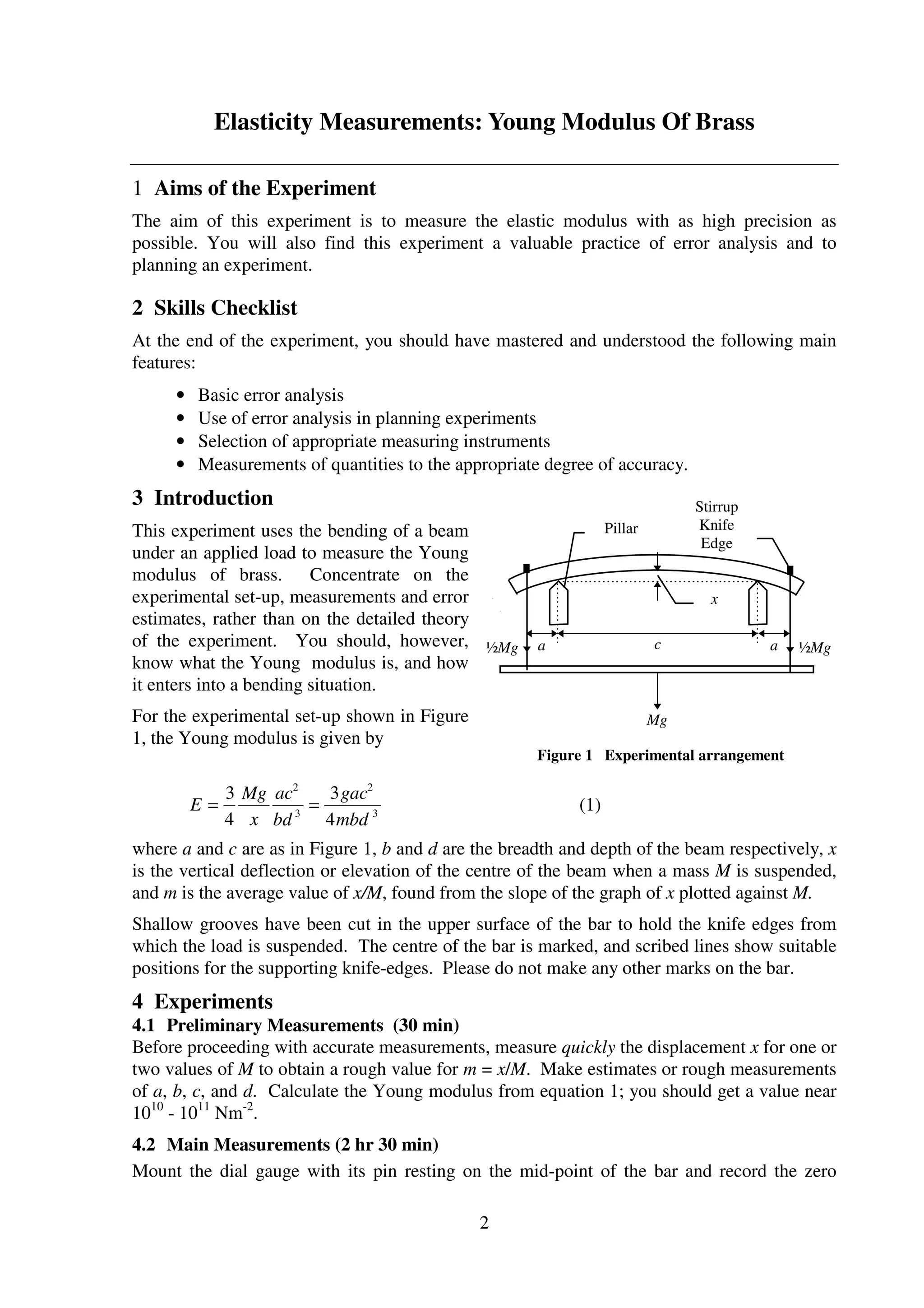
The document provides instructions for an experiment to measure the Young's modulus of brass using beam bending. Students are asked to: 1) Take preliminary measurements of a beam's deflection under different loads to estimate the Young's modulus. 2) Precisely measure the beam's deflection under varying loads and use the slope of a deflection vs. load graph to calculate Young's modulus. 3) Use error analysis to plan further measurements of beam dimensions to achieve a desired accuracy for calculating Young's modulus.

1. 1
Course 1 Laboratory
Second Semester
Experiment:
Young’s Modulus

2. 2
Elasticity Measurements: Young Modulus Of Brass
1 Aims of the Experiment
The aim of this experiment is to measure the elastic modulus with as high precision as
possible. You will also find this experiment a valuable practice of error analysis and to
planning an experiment.
2 Skills Checklist
At the end of the experiment, you should have mastered and understood the following main
features:
• Basic error analysis
• Use of error analysis in planning experiments
• Selection of appropriate measuring instruments
• Measurements of quantities to the appropriate degree of accuracy.
3 Introduction
This experiment uses the bending of a beam
under an applied load to measure the Young
modulus of brass. Concentrate on the
experimental set-up, measurements and error
estimates, rather than on the detailed theory
of the experiment. You should, however,
know what the Young modulus is, and how
it enters into a bending situation.
For the experimental set-up shown in Figure
1, the Young modulus is given by
E
Mg
x
ac
bd
gac
mbd
= =
3
4
3
4
2
3
2
3
(1)
where a and c are as in Figure 1, b and d are the breadth and depth of the beam respectively, x
is the vertical deflection or elevation of the centre of the beam when a mass M is suspended,
and m is the average value of x/M, found from the slope of the graph of x plotted against M.
Shallow grooves have been cut in the upper surface of the bar to hold the knife edges from
which the load is suspended. The centre of the bar is marked, and scribed lines show suitable
positions for the supporting knife-edges. Please do not make any other marks on the bar.
4 Experiments
4.1 Preliminary Measurements (30 min)
Before proceeding with accurate measurements, measure quickly the displacement x for one or
two values of M to obtain a rough value for m = x/M. Make estimates or rough measurements
of a, b, c, and d. Calculate the Young modulus from equation 1; you should get a value near
1010
- 1011
Nm-2
.
4.2 Main Measurements (2 hr 30 min)
Mount the dial gauge with its pin resting on the mid-point of the bar and record the zero
Mg
½Mg½Mg ca a
x
Stirrup
Knife
Edge
Pillar
Figure 1 Experimental arrangement

3. 3
reading. Hang the mass holder from the mid-point of the bar passing through the lower ends
of the stirrups which hang from the beam. Measure the resulting vertical deflection x. Take a
series of measurements of x for masses M up to 6 kg. Then take readings while the bar is
unloaded to check for reproducibility. What should you do if the readings do not reproduce
exactly? Check the positions of the knife edges frequently, and that they remain square.
Plot a graph of x against M on mm graph paper whilst you are taking the results, not
afterwards: this will enable you to spot "rogue" results immediately they arise, and you can
check them at once. Use the Mathcad least squares fitting spreadsheet to find the best value of
m and its error.
You will find that the experimental points do not all lie exactly on the straight line. To
investigate these deviations, measure the deflection x for a mass of about 2-3 kg. Make
several measurements at this mass, unloading and replacing the mass between each reading.
Use Excel to calculate the mean value of x, and to estimate the standard deviation of the
observations about the mean, σ(x), NOT the standard deviation (standard error) of the mean,
u(x).
Since each point on the graph was obtained by measuring one value of x for each value of M,
so the error in x for any one of these points should be the error in x when only one reading of x
is made, and this is σ(x). Put errors bars equal to ±σ(x) on each point of your graph. About
2/3 of the error bars should intersect the best-fit straight line; is this true for your results?
What can you say if all the error bars intersect the line? What can you say if only a few of the
error bars intersect the line? What is your value of χ2
and how does that relate to the above
observations?
Another (very rough) check on your results can be made. The computer will give a value for
the error in m, σ(m). However, assuming that the error in M is negligible, and that there are p
points on your graph, then the fractional error in m, σ(m)/m, is roughly 1/√p times the
fractional error in x, σ(x)/x. Use both methods to estimate σ(m); the two values should agree
to within a factor of 2 or so.
The checks described above are examples of consistency checks. If the different methods do
not agree, then something is wrong somewhere. Unfortunately, agreement does not guarantee
that nothing is wrong!
4.3 Completing the Experiment (1 hr)
The object of this part is to use the theory of propagation of errors as an aid in planning the
rest of the experiment, and then to use these results in measuring the remaining variables to an
appropriate accuracy using an appropriate instrument which you have selected on the basis of
your results.
The fractional error in E in terms of the fractional errors in m, a, b, c and d is
( ) ( ) ( ) ( ) ( ) ( )σ σ σ σ σ σE
E
m
m
a
a
b
b
c
c
d
d





 =





 +





 +





 +





 +






2 2 2 2 2 2
2 3 (2)
For maximum efficiency the percent errors in m, a, b, c², and d3
should be equal, i.e. the five
terms on the RHS of eq. (2) should be the same. But you have a value for one of these terms!
So knowing the percent error in m, use equation (2) to estimate the errors σ(a) etc. you want
in a, b, c, and d. What error in E would you expect to get at the end of the experiment?
Given that the resolution of a wood rule is 1mm, that of a good steel rule is 0.1mm, that of
micrometer screw gauge is 0.001mm (1µm),Vernier callipers is 0.02 mm and that of a

4. 4
select the appropriate instrument to make accurate measurements of a, b, c, and d
Make accurate measurements of a, b, c, and d, and find the errors in these values. The
following points should be noted.
1. Make and record repeated measurements. Use Excel to analyse your results. The errors
you want here are the standard errors of the means, NOT the standard deviations. The
estimates of errors that you have made before are targets, and it may not be possible to
reach them with the equipment you have available. Do not try to better any target unless
you can improve on all of them with little effort! Calculate the error in c² and d3
from the
errors in c and d.
2. When measuring b and d, check the beam for uniformity. Does it matter if the beam is
non-uniform outside the supports?
3. When you use a micrometer, use the ratchet mechanism to tighten the jaws; do not twist the
main barrel. Unless you are a skilled operator, using the barrel will give erratic results, and
you may damage the object being measured if it is squashed too fiercely. Remember it is
possible to read a micrometer to 0.1 of the smallest graduation on its barrel.
4. Use equation (1) to calculate the Young modulus of the brass. Use equation (2) to find the
error in your value of E, using the actual errors you have just found, not the target estimates
from the earlier work!
5 Discussion
1. The beam provided is made of brass. Compare your results with values of E for brass
given in books of tables. Take the experimental uncertainty in your value of E into
account.
2. Sketch a bent beam and mark the regions of tensile and compressive strains. Show the
stresses producing these strains; do they form a couple? Use your sketch to explain why
bending a beam allows the measurement of the tensile Young modulus.
3. Consider the advantages and disadvantages of this method compared with the direct
stretching of the beam or a wire of the same material. Can you think of any other ways of
measuring the Young modulus?
4. What are the main sources of error in E? Is the limit to your accuracy variation due to e.g.
non-uniformity or to the precision of your measuring equipment? Is it feasible, bearing in
mind the time and equipment available, to reduce these errors? Is it really essential to
reduce the errors?
5. Equation (1) relates the elevation per unit mass x/M to the lengths a and c. It is clear that
x/M=0 for a=0 or c=0, and therefore for a beam of fixed length (c+2a) there must be a
value of c for which x/M is a maximum. If you have time, show that this is achieved when
c=4a. Why should you choose c and a to satisfy this relation? Does it matter if c is not
exactly equal to 4a?
6 References
Newman F.H., Searle V.H.L., The General Properties of Matter, 5th edition, (Edward
Arnold, London) 1957.

5. 5
Sprackling M.T., Liquids and Solids, (Routledge and Kegan Paul, London) 1985.
7 Appendix 1
These notes summarise the general forms of the response of a solid body to applied forces.
Further details can be found in Sprackling, chapter 2, or Newman and Searle, chapter 5.
7.1 Elastic Moduli
The moduli of elasticity of a material are measures of its resistance to a change of size or
shape under the influence of a set of applied forces. The applied forces constitute stresses,
expressed as a force per unit area, and the resulting deformation is described as a strain, which
is the ratio of the change in some dimension to an original dimension. If the strain returns to
zero when the stress is removed, the deformation is said to be elastic. In many materials for
small elastic strains, the deformation obeys Hooke's law which states that the stress is
proportional to the strain. The constant of proportionality is the elastic modulus, so that
Modulus = stress/strain
Area A
F
F
F
F
ϕ
δll
Cross-sectional
area A
Figure 2 Shear modulus and Young modulus
Materials can be deformed in several different ways, corresponding to different moduli of
elasticity. For isotropic materials (i.e. those whose properties are the same in all directions)
there are three moduli of particular importance.
1. The bulk modulus, K, corresponds to a change of volume without change of shape. This
applies to deformation under a uniform hydrostatic pressure, The stress is the pressure p,
and the strain is the change in volume -δV (negative because increase in pressure produces
a decrease in volume) divided by the initial volume V. The bulk modulus is given by K =
p/(-δV/V) .
2. The shear modulus, n, also known as the modulus of rigidity, corresponds to a change of
shape at constant volume. The stress is the tangential force F acting over a surface of area
A divided by A, and the strain is represented by the angle of shear, φ. The modulus is given
by n = (F/A)/φ.
3. Young modulus, E, is used when a change in length of a sample is produced when a
tensile or compressive stress is applied, with no external forces applied to the side surfaces
of the specimen. The stress is the tensile force divided by the cross-sectional area of the
sample, and the strain is the change in length δl divided by the original length l, The
modulus is given by E = (F/A)/(δl/l).
At the same time, there is also a contraction or expansion at right angles to the tensile or
compressive stress. The ratio of the magnitude of this transverse strain to the principal strain
is called the Poisson ratio, σ.

6. 6
These various moduli are related by the equations
( ){ }
K
E
=
−3 1 σ
and
( ){ }
n
E
=
+2 1 σ
.
All types of elastic deformation of isotropic media can be described in terms of any two of
these moduli. Note however that an elastic modulus only has meaning if Hooke's law is
obeyed; the ratio stress/strain is not constant for a non-linear material, even if it is perfectly
elastic.
7.2 Theory of A Bending Beam
When a beam is bent into an arc of radius R, the material in one part of the beam is stretched
and under tension, and the material in another part is under compression. These tensile and
compressive strains are produced by related stresses, which combine to form a couple called
the bending moment G. R and G are obviously related to each other, and a little thought
should convince you that the Young modulus of the material, E, and the shape of the bar are
also involved. The full theory of the elastic bending of a beam or cantilever is given in
Newman and Searle (section 5.9). There it is shown (eq. 5.12) that E is given by
E
GR
I
= (A1)
where I, called the second moment of area, is the factor that takes account of the shape of the
bar. (Newman and Searle use the symbol Y for the Young Modulus. They call the second
moment of area I the geometrical moment of inertia, and they use the combination Ak² for
this.) In this experiment, the bending moment is constant along the length AB of the beam,
and its value is
G Mga=
1
2
(A2)
From the geometry of a circle, it can be shown that the radius R is related to the elevation x of
the mid-point by
R
c
x
=
8
(A3)
provided that x is much smaller than R
For a rectangular beam of thickness d and width b, the second moment of area I about its
neutral axis is
I b y y
bd
d
d
= =
−
∫ 2
2
2 3
12
d
/
/
(A4)
Substituting expressions (2), (3) and (4) into (1) gives an expression for the Young modulus in
terms of easily measurable quantities:
E
Mgac
xbd
gac
bd m
= =
3
4
3
4
2
3
2
3 (A5)
where m is the average value of x/M. This is equation (1) of the main text.