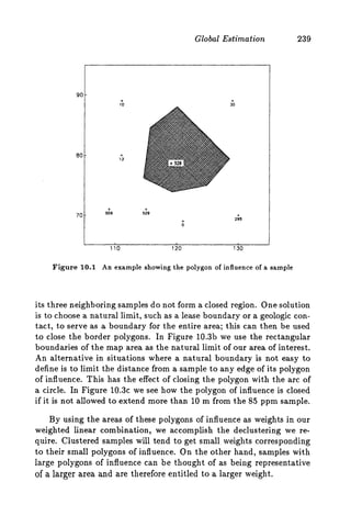
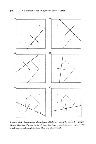
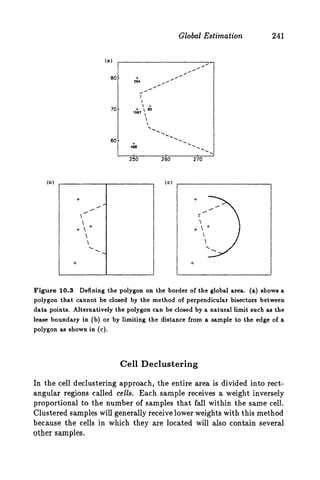
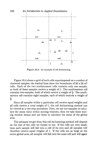
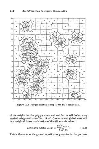
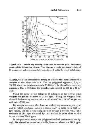
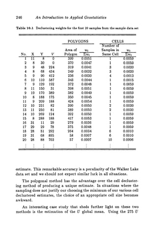
This document discusses two methods for declustering sample data to obtain a better estimate of the global mean: polygonal declustering and cell declustering. Polygonal declustering assigns each sample a polygon of influence based on its proximity to neighboring samples. The area of each polygon is used as the sample's declustering weight. Cell declustering divides the area into rectangular cells, with each sample receiving a weight inversely proportional to the number of samples in its cell. These methods are applied to sample data from Walker Lake to estimate the global vanadium and uranium means. Polygonal declustering performs better for vanadium, while both methods estimate uranium poorly due to sparse sampling in

1. 10
GLOBAL ESTIMATION
When we calculated the sample statistics in Chapter 6 we noticed that
the naive sample mean was a very poor estimate of the exhaustive
mean. Further analysis revealed that the sampling strategy caused our
samples to be preferentially located in areas with high V values. For
example, more than 125 of the 470 samples, for example, fall within the
Wassuk Range anomaly. While it is likely that these samples give good
information on the exhaustive mean within this anomaly, they are not
representative of the remaining area. Unfortunately, the remaining
area is not as densely sampled as the Wassuk Range anomaly. To
obtain a good estimate of the exhaustive mean, we will need to find
some way of weighting individual samples so that the clustered ones
do not have an undue influence on our estimate.
We have already seen in Table 6.2 that if we use only the 195
samples from the initial campaign, our sample mean is much closer
to the actual exhaustive value than if we include the samples from
the second and third campaigns. A weighted linear combination that
gives equal weight to the first 195 sample values and no weight to the
last 275 produces a better estimate of the global mean than one that
weights all 470 sample equally.
This method of giving no weight to the clustered samples has two
drawbacks. First, it completely ignores useful information. We should
not discard the measurements from our 275 clustered samples; instead,
we should try to find some way to moderate their influence. Second,
it may not always be possible to identify those samples that should

2. 238 An Introduction to Applied Geostatistics
be kept and those that should be discarded. We are fortunate with
the Walker Lake sample data set in being able to identify the three
sampling campaigns. In practice, we may not be able to find a natural
subset of samples that completely covers the area on a pseudo regular
grid.
In this chapter we look at two declustering methods that are gen-
erally applicable to any sample data set. In both methods we use a
weighted linear combination of all available sample values to estimate
the exhaustive mean. By assigning different weights to the available
samples, we can effectively decluster the data set. The first method,
called the polygonal method, assigns a polygon of influence to each
sample. The areas of these polygons are then used as the declustering
weights. The second method, called the cell declustering method, uses
the moving window concept to calculate how many samples fall within
particular regions or cells. The declustering weight assigned to a sam-
ple is inversely proportional to the number of other samples that fall
within the same cell. Following a detailed description of how these two
methods are implemented, we will see how both methods perform on
the Walker Lake data set.
PoIygona1 Dec1usteri11g
Each sample in our data set has a polygon of influence within which
it is closer than any other sample. Figure 10.1 shows the locations
of some arbitrary samples. The shaded area shows the polygon of
influence for the 328 ppm sample located near the center of this area.
Any point within the shaded region is closer to the 328 ppm sample
than to any other.
Figure 10.2 shows how the boundaries of the polygon of influence
are uniquely defined. The perpendicular bisector of a line segment is a
line on which points are equidistant from either end of the line segment;
points on either side of the perpendicular bisector have to be closer to
one end or the other. The perpendicular bisectors between a sample
and its neighbors form the boundaries of the polygon of influence.
The edges of the global area require special treatment. A sample
located near the edge of the area of interest may not be completely
surrounded by other samples and the perpendicular bisectors with its
neighbors may not form a closed polygon. Figure 10.3a shows an exam-
ple where the perpendicular bisectors between the 85 ppm sample and

3. Global Estimation 239
+ +
10 30
Figure 10.1 An example showing the polygon of influence of a sample
its three neighboring samples do not form a closed region. One solution
is to choose a natural limit, such as a lease boundary or a geologic con-
tact, to serve as a boundary for the entire area; this can then be used
to close the border polygons. In Figure 10.3b we use the rectangular
boundaries of the map area as the natural limit of our area of interest.
An alternative in situations where a natural boundary is not easy to
define is to limit the distance from a sample to any edge of its polygon
of influence. This has the effect of closing the polygon with the arc of
a circle. In Figure 1 0 . 3 ~we see how the polygon of influence is closed
if it is not allowed to extend more than 10 m from the 85 ppm sample.
By using the areas of these polygons of influence as weights in our
weighted linear combination, we accomplish the declustering we re-
quire. Clustered samples will tend to get small weights corresponding
to their small polygons of influence. On the other hand, samples with
large polygons of influence can be thought of as being representative
of a larger area and are therefore entitled to a larger weight.

4. 240
(
A n Introduction to Applied Geostatistics
Figure 10.2 Construction of a polygon of influence using the method of perpen-
dicular bisectors. Figures (a) to (f) show the steps in constructing a region within
which the central sample is closer than any other sample.

5. Global Estimation 241
Figure 10.3 Defining the polygon on the border of the global area. (a) shows a
polygon that cannot be closed by the method of perpendicular bisectors between
data points. Alternatively the polygon can be closed by a natural limit such as the
lease boundary in (b) or by limiting the distance from a sample to the edge of a
polygon as shown in (c).
Cell Declustering
In the cell declustering approach, the entire area is divided into rect-
angular regions called cells. Each sample receives a weight inversely
proportional to the number of samples that fall within the same cell.
Clustered samples will generally receive lower weights with this method
because the cells in which they are located will also contain several
other samples.

6. 242 A n .Introduction to Applied Geostatistics ,
I I I
I I I
---L--------_---~-------------~---
I I I
I I I
I I I
I I I
I I I
I I I
I I I
I
+
316
I
I
I+
10
I
(533 6 + I
13 +
4 8 I 328
I
I + + I
+ I +
I
I
I 325 I 0
I I I
I I I
II
I I
I I + +
I I 0 273 I
1 ; 2:6 506 529
I n=2 I n=8 I
I+
___-___-____-___-_________________
304
Figure 10.4 An example of cell declustering.
Figure 10.4 shows a grid of such cells superimposed on a number of
clustered samples; the dashed lines show the boundaries of 20 x 20 m2
cells. Each of the two northernmost cells contains only one sample,
so both of these samples receive a weight of 1. The southwestern cell
contains two samples, both of which receive a weight of $.The south-
eastern cell contains eight samples, each of which receives a weight of
8.
Since all samples within a particular cell receive equal weights and
all cells receive a total weight of 1, the cell declustering method can
be viewed as a two step procedure. First, we use our samples to calcu-
late the mean value within moving windows, then we take these mov-
ing window means and use them to calculate the mean of the global
area.
Tlie estimate we get from this cell declustering method will depend
on the size of the cells we choose to use. If the cells are very small,
then each sample will fall into a cell of its own and all samples will
therefore receive equal weights of 1. If the cells are as large as the
entire global area, all samples will fall into the same cell and will again
1

7. Global Estimation 243
receive equal weights. Somewhere between these two extremes we must
find an appropriate medium.
If there is an underlying pseudo regular grid, then the spacing of
this grid usually provides a good cell size. In our Walker Lake example,
the sampling grid from the first program suggests that 20 x 20 m2 cells
would adequately decluster our data. If the sampling pattern does not
suggest a natural cell size, a common practice is to try several cell
sizes and to pick the one that gives the lowest estimate of the global
mean. This is appropriate if the clustered sampling is exclusively in
areas with high values. In such cases, which are common in practice,
we expect the clustering of the samples to increase our estimate of the
mean, so we are justified in choosing the cell size that produces the
lowest estimate.
Comparison of Declustering Methods
Having discussed how the two declustering methods are implemented,
we can now try them both on our Walker Lake sample data set. We
will estimate the global V mean using the 470 V samples. From our
description of the exhaustive data set in Chapter 5 we know that the
true value is 278 ppm. Though the case study here aims only at the
estimation of the global mean, we will see later that the declustering
weights we calculate here can also be used for other purposes. In
Chapter 18, we will take a look at estimating an entire distribution
and its various declustered statistics.
The polygons of influence for the Walker Lake sample data set
are shown in Figure 10.5. In this figure we have chosen to use the
rectangular boundaries of the map area to close the border polygons.
For the cell declustering method we must choose an appropriate
cell size. Since we are using rectangular cells we can vary both the
east-west width and the north-south height of our cells. In Figure 10.6
we have contoured the estimated global means we obtain using cells
of different sizes. The minimum on this map occurs for a cell whose
east-west dimension is 20 m and north-south dimension is 23.08 m.
We are justified in choosing this minimum over all other possibilities
since our clustered samples are all located in areas with high V values.
This 20 x 23 m2cell size also nearly coincides with the spacing of the
pseudo regular grid from the first sampling campaign.
For the first 20 samples, Table 10.1 gives details of the calculation

8. 244 A n Introduction to Applied Ceostatistics
0
Figure 10.5 Polygon of influence map for the 470 V sample data.
of the weights for the polygonal method and for the cell declustering
method using a cell size of 20 x 23 m2. Our estimated global mean will
be a weighted linear combination of the 470 sample values:
xg;w;* vi
c;L; wj
Estimated Global Mean = (10.1)
This is the same as the general equation we presented in the previous

9. Global Estimation 245
Size of cells in E-W direction
Figure 10.6 Contour map showing the relation between the global declustered
mean and the declustering cell size. From this map it can be seen that a cell size of
20 m east-west and approximately 23 m north-south yields the lowest global mean.
chapter, with the denominator acting as a factor that standardizes the
weights so that they sum to 1. For the polygonal approach, C W j =
78,000 since the total map area is 78,000 m2; for the cell declustering
approach, Cwi = 169 since the global area is covered by 169 20 x 23 m2
cells.
Using the areas of the polygons of influence as our declustering
weights we get an estimate of 276.8 ppm. Using the weights from
the cell declustering method with a cell size of 20 x 23 m2 we get an
estimate of 288 pm.
For sample data sets that have an underlying pseudo regular grid
and in which clustered sampling occurs only in areas with high or
low values, the cell declustering method usually performs well. The
estimate of 288 ppm obtained by this method is quite close to the
actual value of 276.9 ppm.
In this particular study, the polygonal method performs extremely
well, We should be somewhat humble, however, about our 276.8 pprn

10. 246 An Introduction to Applied Geostatistics
Table 10.1 Declustering weights for the first 20 samples from the sample data set
POLYGONS CELLS
Number of
Area of wi Samples in wi
No. X Y V Polygon Cwj Same Cell Cwi
1 1 1 8 0 399 0.0051 1 0.0059
2 8
3 9
4 8
5 9
6 10
7 9
8 11
9 10
10 8
11 9
12 10
13 11
14 10
15 8
16 31
17 29
18 28
19 31
20 28
30
48
68
90
110
129
150
170
188
209
231
250
269
288
11
29
51
G8
88
0
224
434
412
587
192
31
389
175
188
82
81
124
188
29
78
292
895
703
370
319
249
236
343
372
398
382
350
424
390
389
392
417
279
375
2G4
58
57
0.0047
0.0041
0.0032
0.0030
0.0044
0.0048
0.0051
0.0049
0.0045
0.0054
0.0050
0.0050
0.0050
0.0053
0.0036
0.0048
0.0034
0.0007
0.0007
1
3
3
4
1
1
1
1
1
1
2
2
1
1
1
1
6
6
10
0.0059
0.0020
0.0020
0.0013
0.0015
0.0059
0.0059
0.0059
0.0059
0.0059
0.0030
0.0030
0.0059
0.0059
0.0059
0.0059
0.0010
0.0010
0.0006
estimate. This remarkable accuracy is a peculiarity of the Walker Lake
data set and we should not expect similar luck in all situations.
The polygonal method has the advantage over the cell decluster-
ing method of producing a unique estimate. In situations where the
sampling does not justify our choosing the minimum of our various cell
declustered estimates, the choice of an appropriate cell size becomes
awkward.
An interesting case study that sheds further light on these two
methods is the estimation of the U global mean. Using the 275 U

11. Global Estimation 247
samples we can repeat the calculation of the declustering weights for
both methods. In this case, the true value is 266 ppm. The polygonal
estimate is 338 ppm while the minimum cell declustering estimate is
473 ppm. In this example both methods fare poorly because there are
large portions of the map area with preferentially low values that have
no U samples. Neither of these methods can hope to replace actual
samples; all they do is make intelligent use of the available samples. It
is worth noting that in this case, where there is no underlying pseudo
regular grid that covers the area, the cell declustering approach pro-
duces a considerably poorer estimate than the polygonal approach.
Declustering Three Dimensional Data
The methods we have presented here work well with two-dimensional
data sets. For the declustering of three-dimensional data sets, there
are several possible adaptations of these tools.
If the data are layered, then one may be able to separate the
data into individual layers and then use a two-dimensional decluster-
ing methods on each layer. If the data set cannot easily be reduced
to several two-dimensional data sets, it is possible to use the three-
dimensional version of either of the methods discussed here.
For the cell declustering approach, the cells become rectangular
blocks whose width, height and depth we must choose. If the appro-
priate dimensions of such blocks are not obvious from the available
sampling, one can still experiment with several block dimensions in an
attempt to find the one that minimizes (or maximizes) the estimate of
the global mean. In three dimensions, however, this procedure is more
tedious and less difficult to visualize than in two.
The three-dimensional analog of the polygonal approach consists
of dividing the space into polyhedra within which the central sample is
closer than any other sample. The volume of each polyhedron can then
be used as a declustering weight for the central sample. An alternative
approach, which is easier to implement though usually more computa-
tionally expensive, is to discretize the volume into many points, and to
assign to each sample a declustering weight that is proportional to the
number of points which are closer to that sample than to any other.
A final alternative, one whose twcldimensional version we have
not yet discussed, is to use the global kriging weights as declustering
weights. In Chapter 20 we will show how these weights can be obtained

12. 248 An Introduction to Applied Geostatistics
by accumulating local kriging weights. If a good variogram model can
be chosen, this final alternative has the advantage of accounting for
the pattern of spatial continuity of the phenomenon.
Further Reading
Hayes, W. and Koch, G. , “Constructing and analyzing area-of-
influence polygons by computer,” Computers and Geosciences,
V O ~ .10, pp. 411-431, 1984.
Journel, A. , “Non-parametric estimation of spatial distributions,”
Mathematical Geology, vol. 15, no. 3, pp. 445-468, 1983.