The document discusses key concepts in probability and their application to archaeological data analysis. It explains that probability can be assessed from both frequentist and Bayesian perspectives. The frequentist view assesses probabilities as objective frequencies of outcomes, while the Bayesian view incorporates prior knowledge. Several probability concepts are defined, including discrete vs. continuous probabilities and independent vs. conditional probabilities. The binomial theorem is introduced for calculating probabilities of outcomes from repeated trials. The document demonstrates how these probability concepts can help archaeologists evaluate sample sizes, absence of artifact types, and differences between sites while accounting for chance.

1. Probability

2. Questions what is a good general size for artifact samples? what proportion of populations of interest should we be attempting to sample? how do we evaluate the absence of an artifact type in our collections?

3. “ frequentist” approach probability should be assessed in purely objective terms no room for subjectivity on the part of individual researchers knowledge about probabilities comes from the relative frequency of a large number of trials this is a good model for coin tossing not so useful for archaeology, where many of the events that interest us are unique…

4. Bayesian approach Bayes Theorem Thomas Bayes 18 th century English clergyman concerned with integrating “prior knowledge” into calculations of probability problematic for frequentists prior knowledge = bias, subjectivity…

5. basic concepts probability of event = p 0 <= p <= 1 0 = certain non-occurrence 1 = certain occurrence .5 = even odds .1 = 1 chance out of 10

6. if A and B are mutually exclusive events: P(A or B) = P(A) + P(B) ex., die roll: P(1 or 6) = 1/6 + 1/6 = .33 possibility set : sum of all possible outcomes ~A = anything other than A P(A or ~A) = P(A) + P(~A) = 1 basic concepts (cont.)

7. discrete vs. continuous probabilities discrete finite number of outcomes continuous outcomes vary along continuous scale basic concepts (cont.)

8. discrete probabilities 0 .25 .5 p HH TT HT

9. continuous probabilities total area under curve = 1 but the probability of any single value = 0  interested in the probability assoc. w/ intervals 0 .1 .2 p 0 .1 .2 p

10. independent events one event has no influence on the outcome of another event if events A & B are independent then P(A&B) = P(A)*P(B) if P(A&B) = P(A)*P(B) then events A & B are independent coin flipping if P(H) = P(T) = .5 then P(HTHTH) = P(HHHHH) = .5*.5*.5*.5*.5 = .5 5 = .03

11. if you are flipping a coin and it has already come up heads 6 times in a row, what are the odds of an 7 th head? .5 note that P(10H) < > P(4H,6T) lots of ways to achieve the 2 nd result (therefore much more probable)

12. mutually exclusive events are not independent rather, the most dependent kinds of events if not heads, then tails joint probability of 2 mutually exclusive events is 0 P(A&B)=0

13. conditional probability concern the odds of one event occurring, given that another event has occurred P(A|B)=Prob of A, given B

14. e.g. consider a temporally ambiguous, but generally late, pottery type the probability that an actual example is “ late ” increases if found with other types of pottery that are unambiguously late … P = probability that the specimen is late: isolated: P(T a ) = .7 w/ late pottery (T b ): P(T a |T b ) = .9 w/ early pottery (T c ): P(T a |T c ) = .3

15. P(B|A) = P(A&B)/P(A) if A and B are independent , then P(B|A) = P(A)*P(B)/P(A) P(B|A) = P(B) conditional probability (cont.)

16. Bayes Theorem can be derived from the basic equation for conditional probabilities

17. application archaeological data about ceramic design bowls and jars, decorated and undecorated previous excavations show: 75% of assemblage are bowls , 25% jars of the bowls , about 50% are decorated of the jars , only about 20% are decorated we have a decorated sherd fragment, but it’s too small to determine its form… what is the probability that it comes from a bowl ?

18. can solve for P(B|A) events:?? events: B = “bowlness”; A = “decoratedness” P(B)=??; P(A|B)=?? P(B)=.75; P(A|B)=.50 P(~B)=.25; P(A|~B)=.20 P(B|A)=.75*.50 / ((.75*50)+(.25*.20)) P(B|A)=.88 25% jar 50% of bowls 80% of jars undec. 75% 50% of bowls 20% of jars ?? dec. bowl

19. Binomial theorem P(n,k,p) probability of k successes in n trials where the probability of success on any one trial is p “ success” = some specific event or outcome k specified outcomes n trials p probability of the specified outcome in 1 trial

20. where n! = n*(n-1)*(n-2)…*1 (where n is an integer) 0!=1

21. misc. useful derivations from BT if repeated trials are carried out: mean successes (k) = n*p sd of successes (k) =  npq (note: q=1-p) (really only approximated when trials are repeated many times…) k=0; P(n,0,p)=(1-p) n

22. binomial distribution binomial theorem describes a theoretical distribution that can be plotted in two different ways: probability density function (PDF) cumulative density function (CDF)

23. probability density function (PDF) summarizes how odds / probabilities are distributed among the events that can arise from a series of trials

24. ex: coin toss we toss a coin three times, defining the outcome head as a “success”… what are the possible outcomes? how do we calculate their probabilities?

25. coin toss (cont.) how do we assign values to P(n,k,p) ? 3 trials; n = 3 even odds of success; p=.5 P(3,k,.5) there are 4 possible values for ‘k’, and we want to calculate P for each of them “probability of k successes in n trials where the probability of success on any one trial is p” HHH 3 H TT (THT,TTH) 1 HH T (HTH, THH) 2 TTT 0 k

27. practical applications how do we interpret the absence of key types in artifact samples?? does sample size matter?? does anything else matter??

28. we are interested in ceramic production in southern Utah we have surface collections from a number of sites are any of them ceramic workshops?? evidence: ceramic “wasters” ethnoarchaeological data suggests that wasters tend to make up about 5% of samples at ceramic workshops example

29. one of our sites  15 sherds, none identified as wasters… so, our evidence seems to suggest that this site is not a workshop how strong is our conclusion??

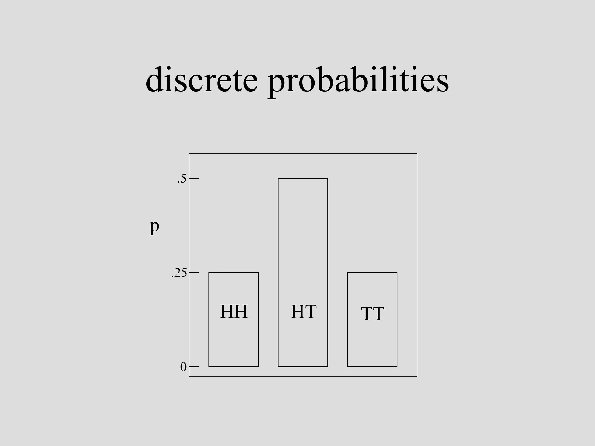
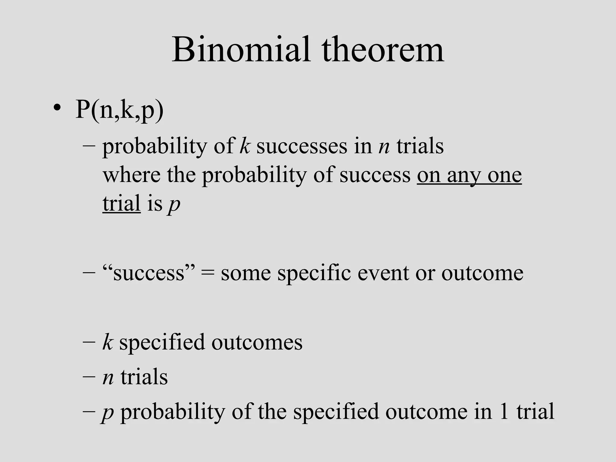
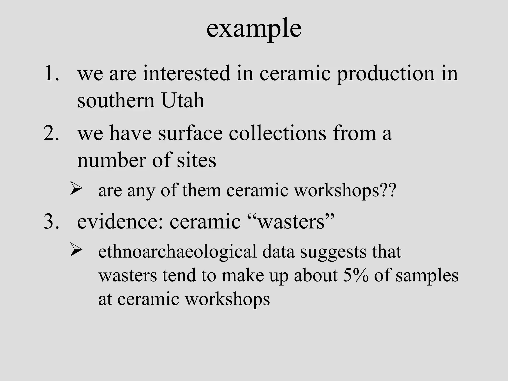
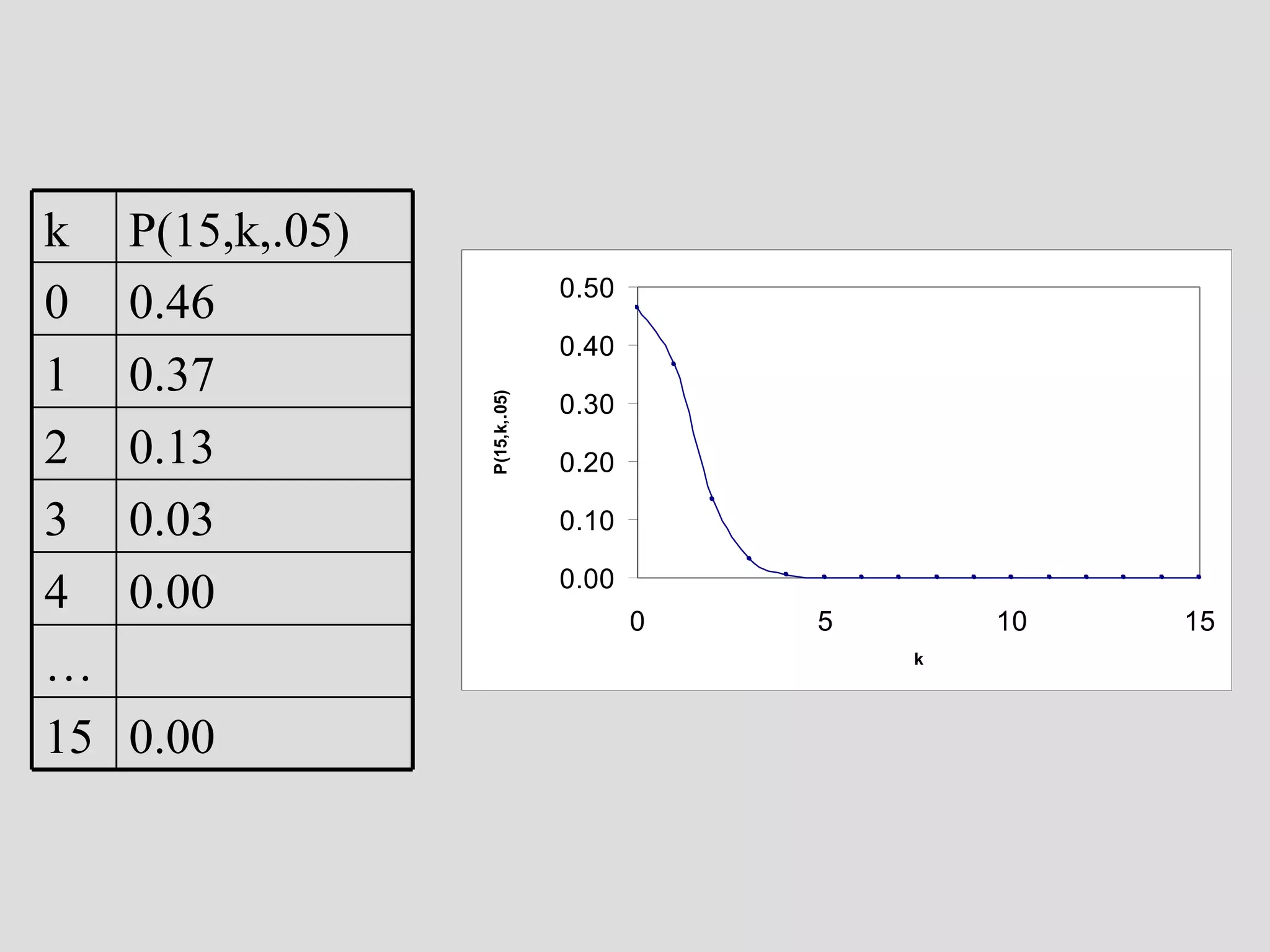
30. reverse the logic: assume that it is a ceramic workshop new question: how likely is it to have missed collecting wasters in a sample of 15 sherds from a real ceramic workshop?? P(n,k,p) [ n trials, k successes, p prob. of success on 1 trial] P(15,0,.05) [we may want to look at other values of k…]

31. … 15 4 3 2 1 0 k 0.00 0.00 0.03 0.13 0.37 0.46 P(15,k,.05)

32. how large a sample do you need before you can place some reasonable confidence in the idea that no wasters = no workshop? how could we find out?? we could plot P( n ,0,.05) against different values of n …

33. 50 – less than 1 chance in 10 of collecting no wasters… 100 – about 1 chance in 100…

34. What if wasters existed at a higher proportion than 5%??

35. so, how big should samples be? depends on your research goals & interests need big samples to study rare items… “rules of thumb” are usually misguided (ex. “200 pollen grains is a valid sample”) in general, sheer sample size is more important that the actual proportion large samples that constitute a very small proportion of a population may be highly useful for inferential purposes

36. the plots we have been using are probability density functions (PDF) cumulative density functions (CDF) have a special purpose example based on mortuary data…

37. Site 1 800 graves 160 exhibit body position and grave goods that mark members of a distinct ethnicity (group A) relative frequency of 0.2 Site 2 badly damaged; only 50 graves excavated 6 exhibit “group A” characteristics relative frequency of 0.12 Pre-Dynastic cemeteries in Upper Egypt

38. expressed as a proportion, Site 1 has around twice as many burials of individuals from “group A” as Site 2 how seriously should we take this observation as evidence about social differences between underlying populations?

39. assume for the moment that there is no difference between these societies—they represent samples from the same underlying population how likely would it be to collect our Site 2 sample from this underlying population? we could use data merged from both sites as a basis for characterizing this population but since the sample from Site 1 is so large, lets just use it …

40. Site 1 suggests that about 20% of our society belong to this distinct social class… if so, we might have expected that 10 of the 50 sites excavated from site 2 would belong to this class but we found only 6…

41. how likely is it that this difference (10 vs. 6) could arise just from random chance ?? to answer this question, we have to be interested in more than just the probability associated with the single observed outcome “6” we are also interested in the total probability associated with outcomes that are more extreme than “6”…

42. imagine a simulation of the discovery/excavation process of graves at Site 2: repeated drawing of 50 balls from a jar: ca. 800 balls 80% black, 20% white on average , samples will contain 10 white balls, but individual samples will vary

43. by keeping score on how many times we draw a sample that is as , or more divergent (relative to the mean sample) than what we observed in our real-world sample… this means we have to tally all samples that produce 6, 5, 4…0, white balls… a tally of just those samples with 6 white balls eliminates crucial evidence…

44. we can use the binomial theorem instead of the drawing experiment, but the same logic applies a cumulative density function (CDF) displays probabilities associated with a range of outcomes (such as 6 to 0 graves with evidence for elite status)

45. 0.103 0.055 0.20 6 50 0.048 0.030 0.20 5 50 0.018 0.013 0.20 4 50 0.006 0.004 0.20 3 50 0.001 0.001 0.20 2 50 0.000 0.000 0.20 1 50 0.000 0.000 0.20 0 50 cumP P(n,k,p) p k n

47. so, the odds are about 1 in 10 that the differences we see could be attributed to random effects—rather than social differences you have to decide what this observation really means, and other kinds of evidence will probably play a role in your decision…