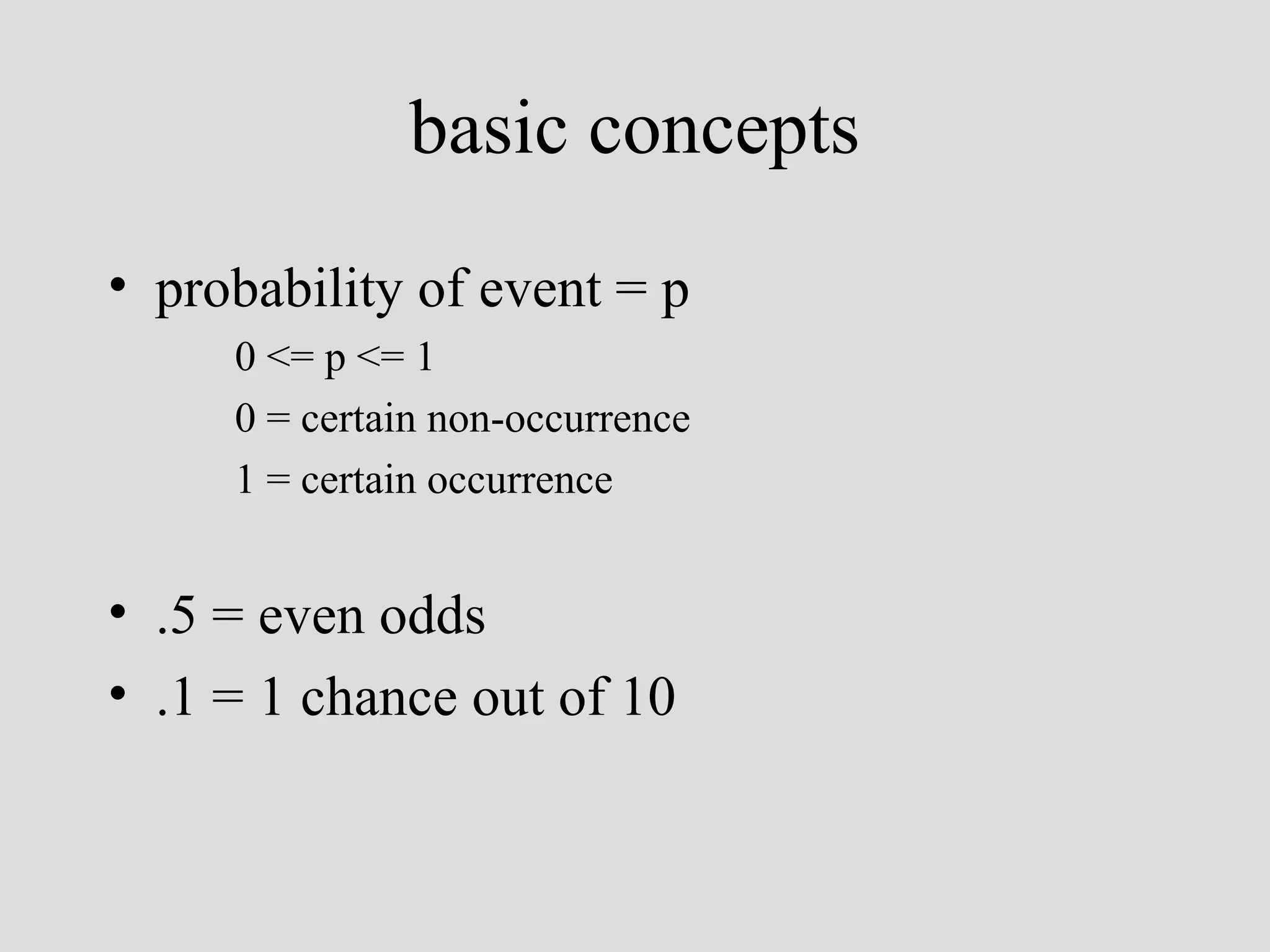
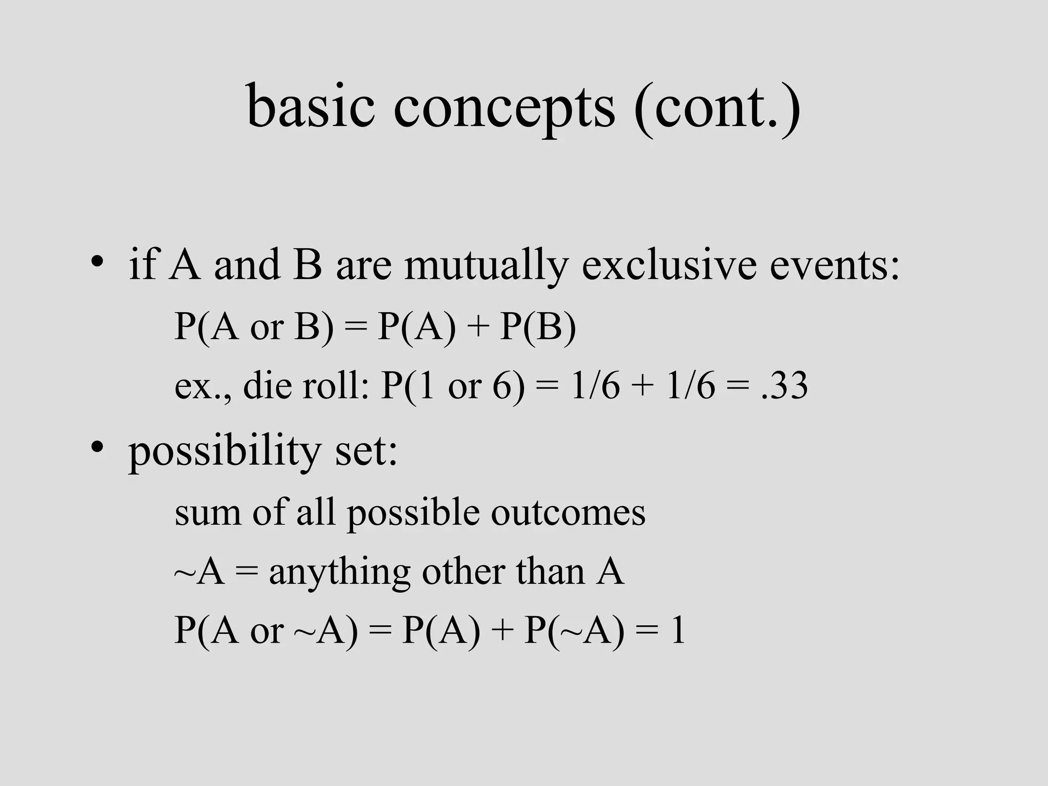
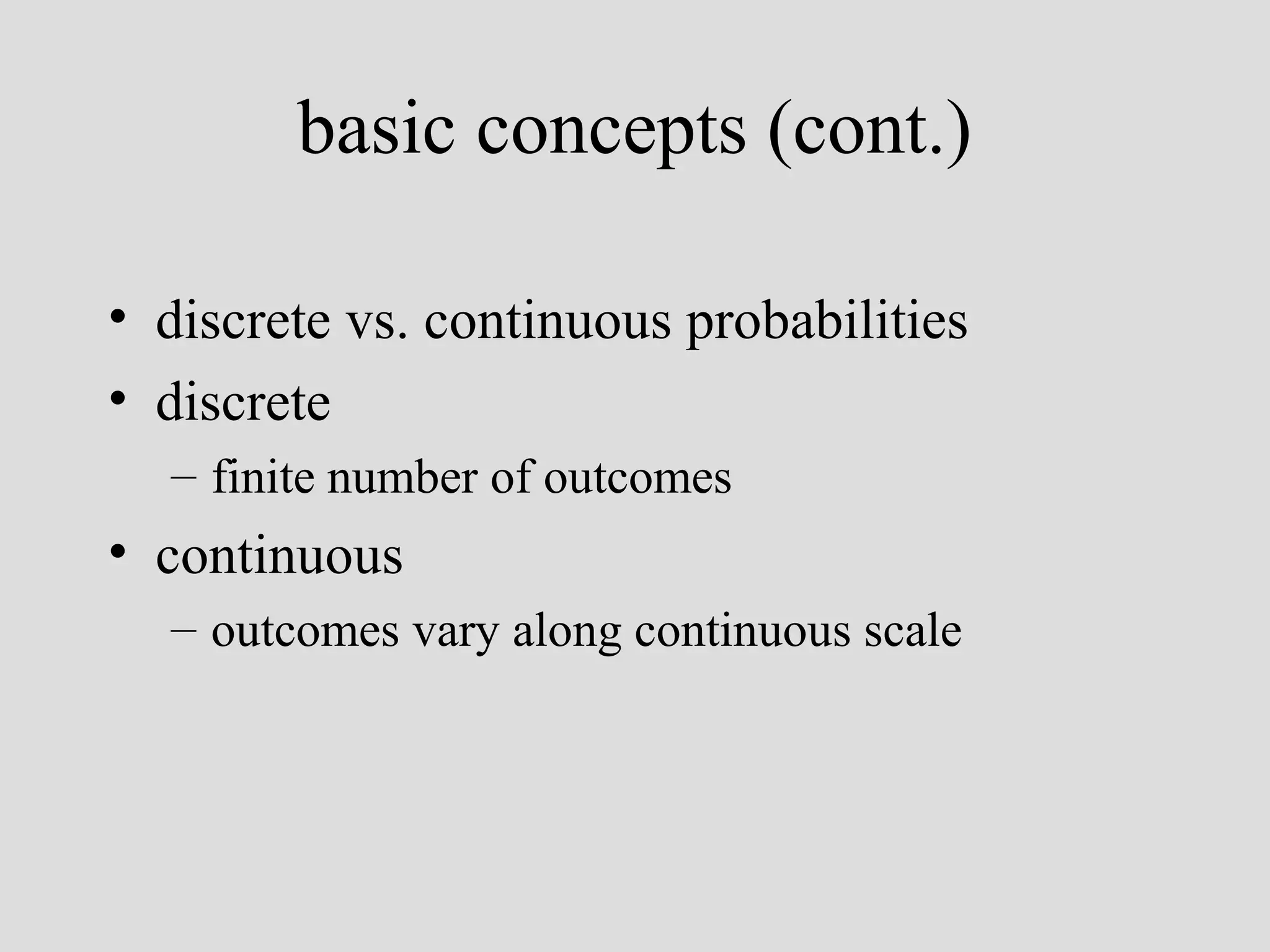
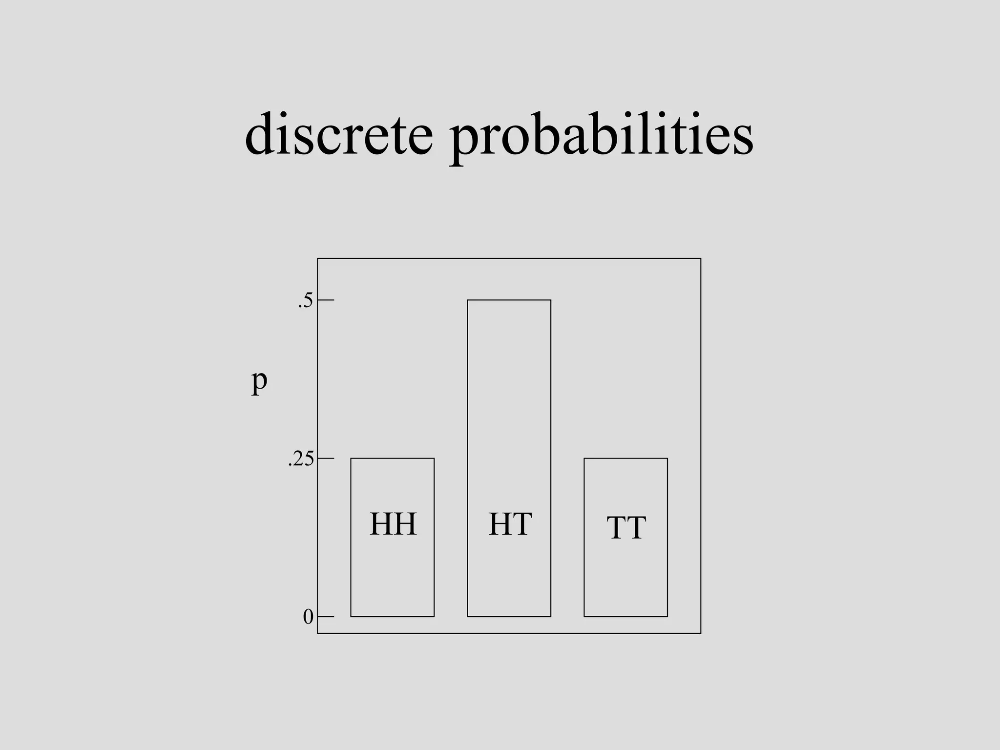
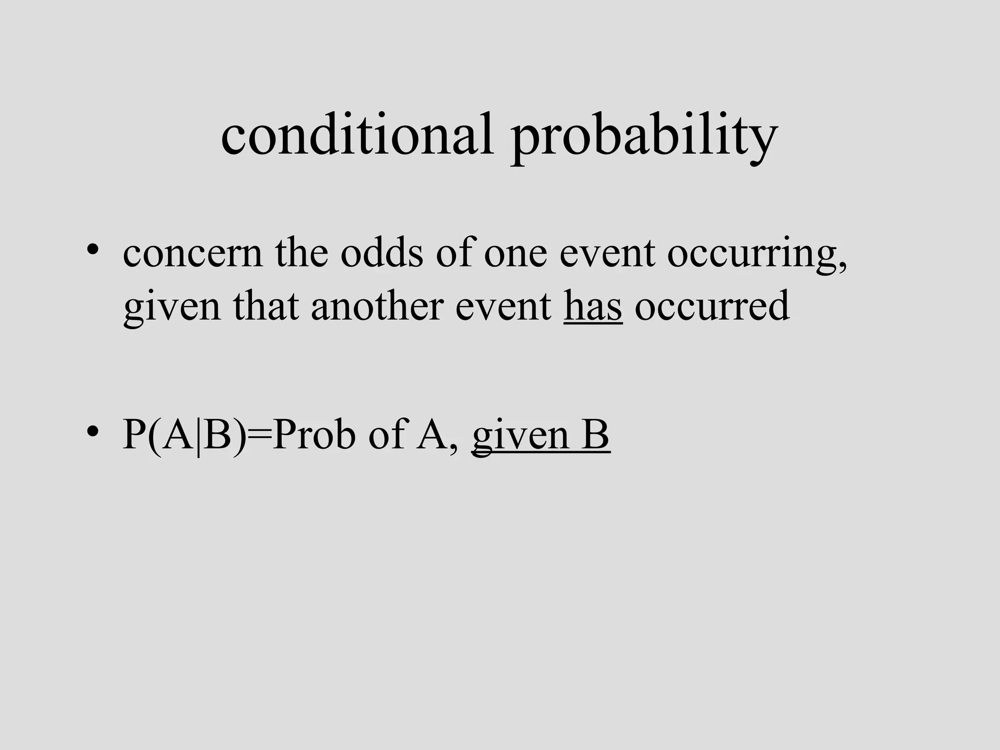
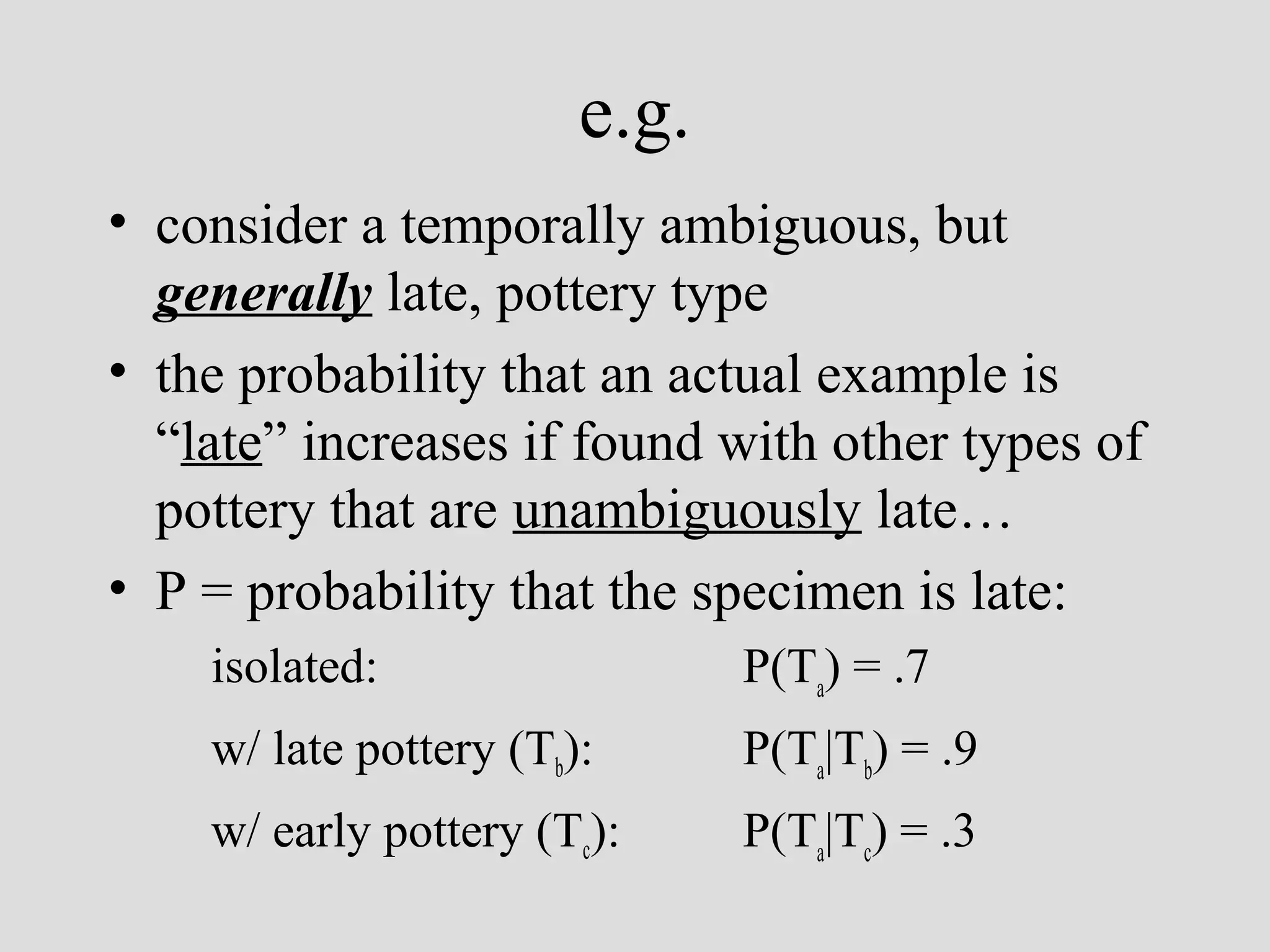
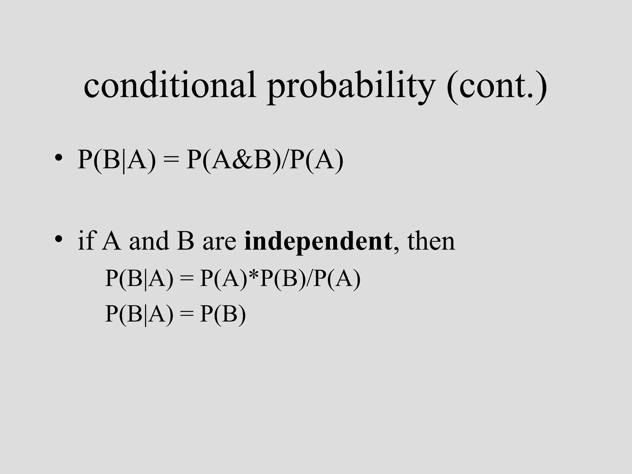
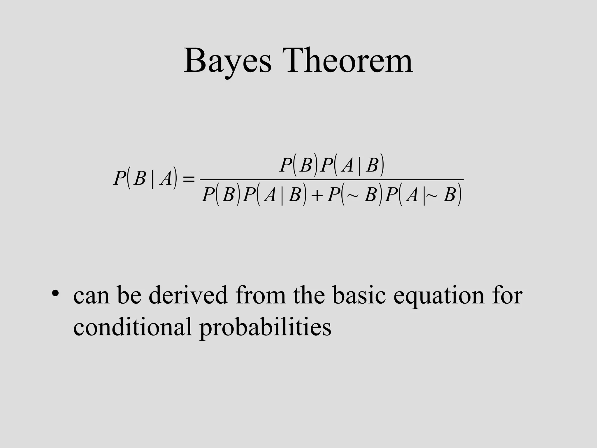
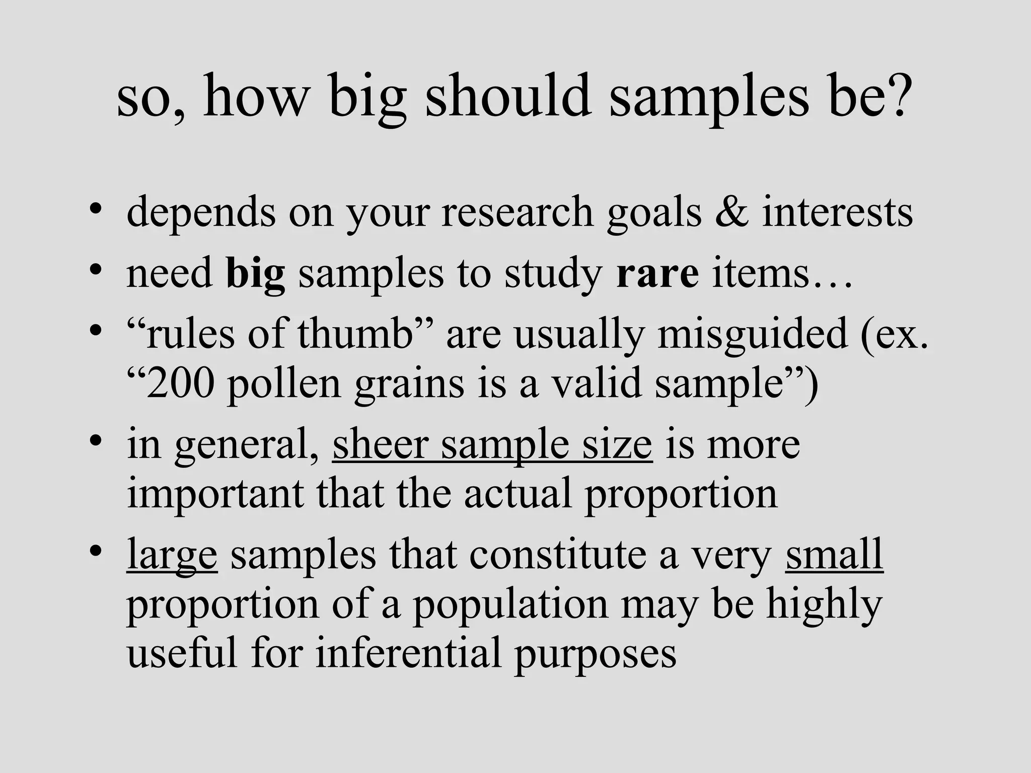
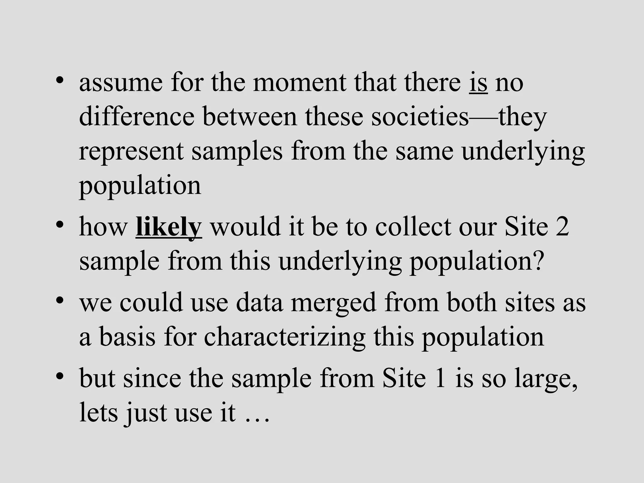
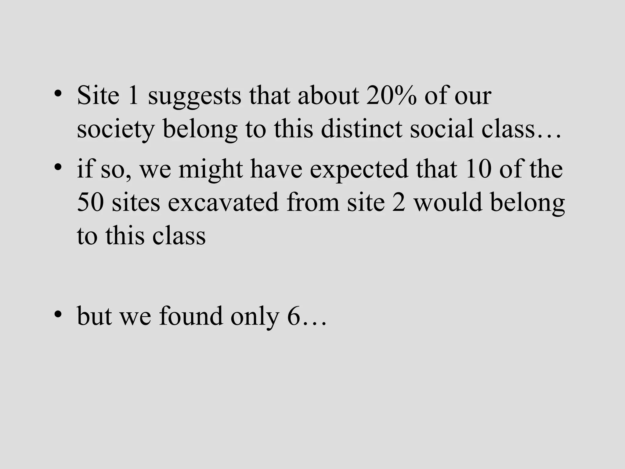
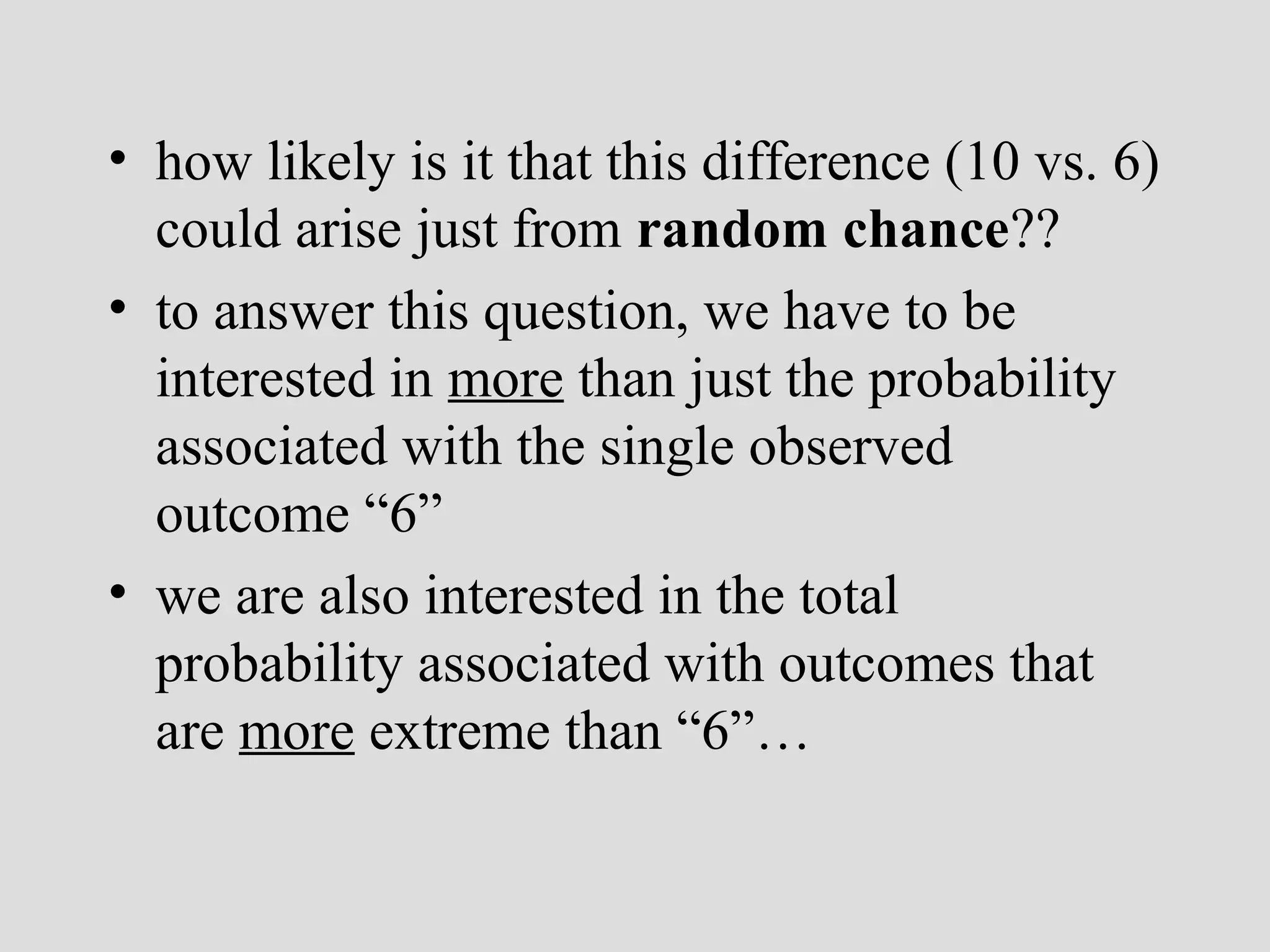
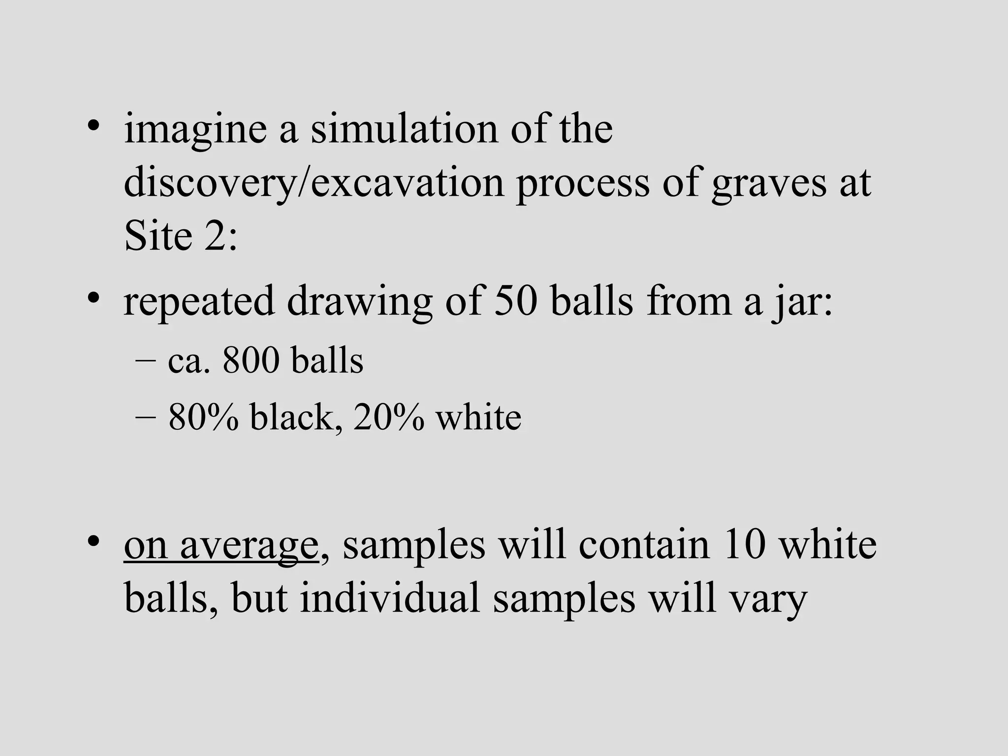
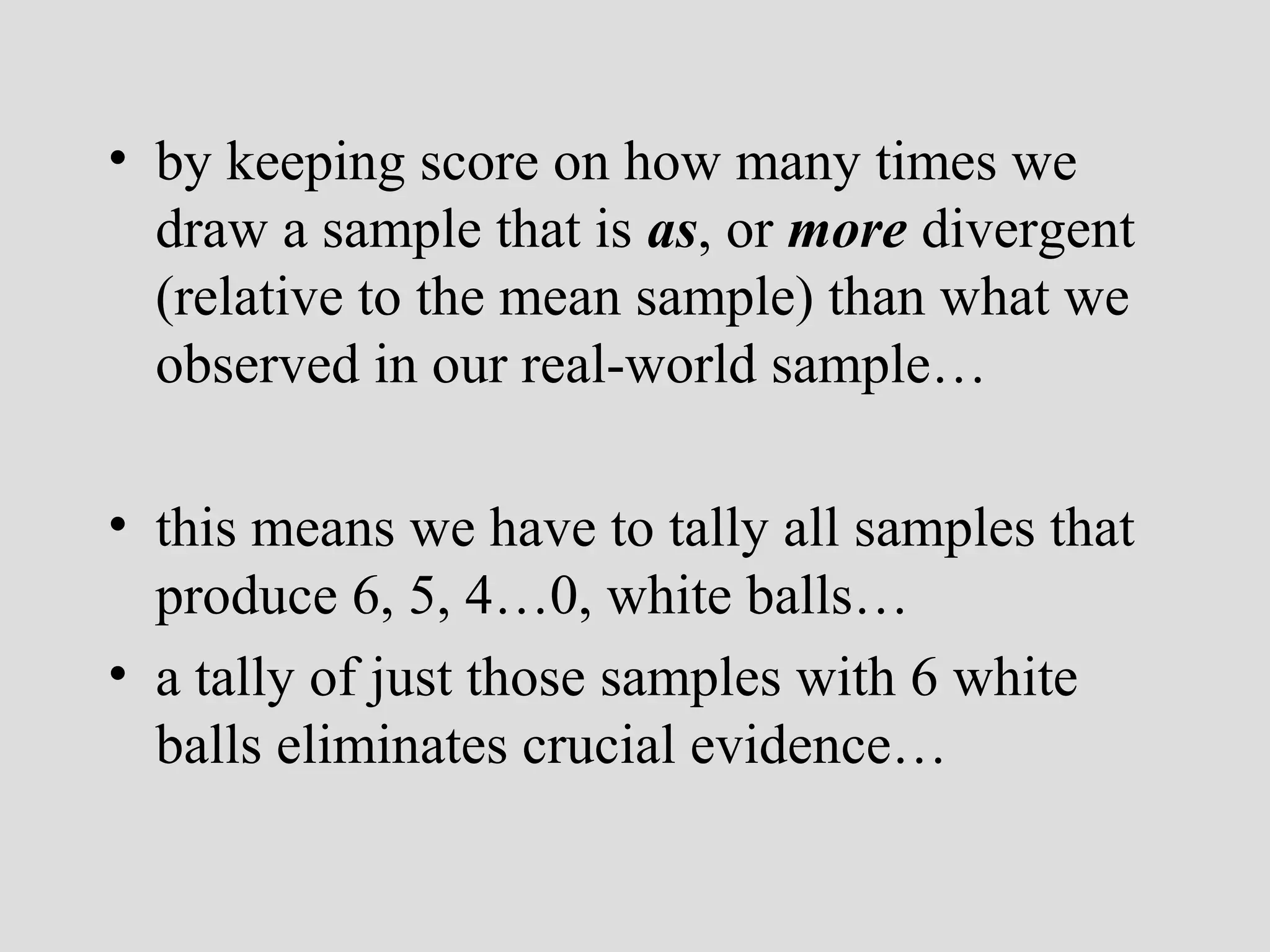
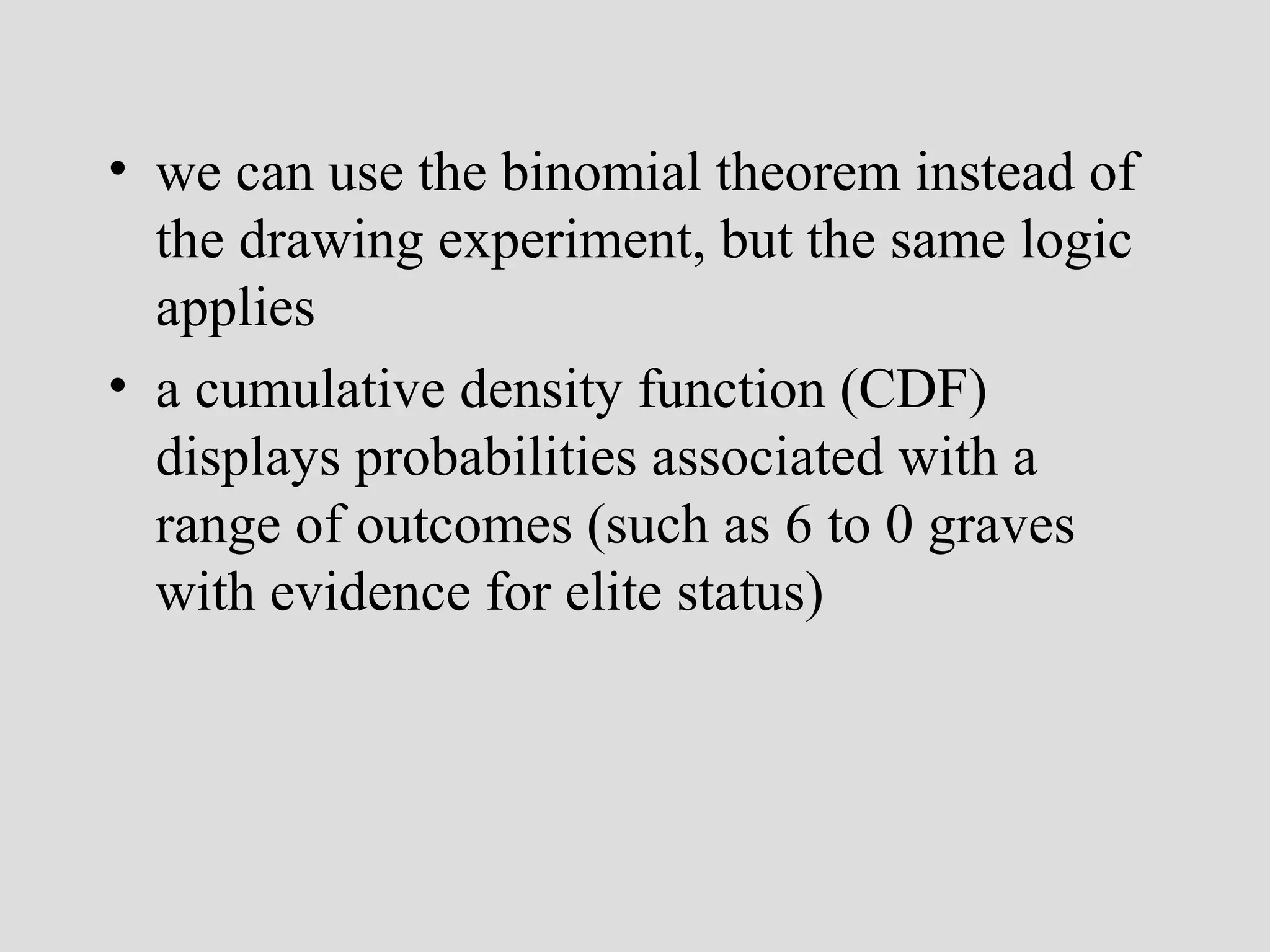
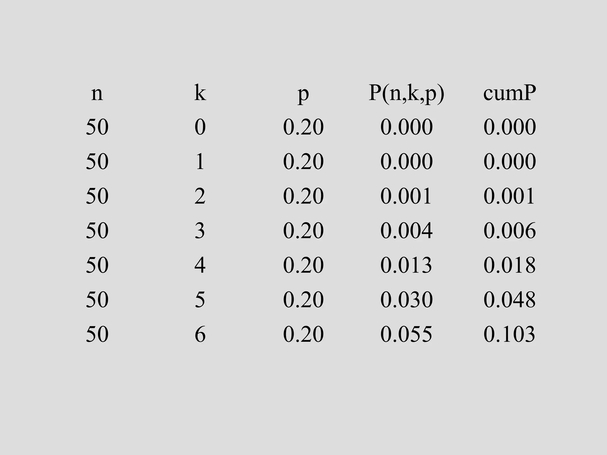
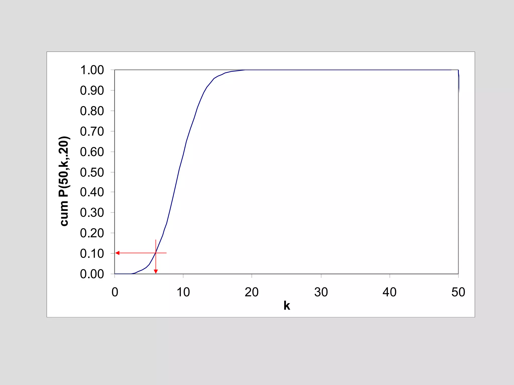
Downloaded 10 times
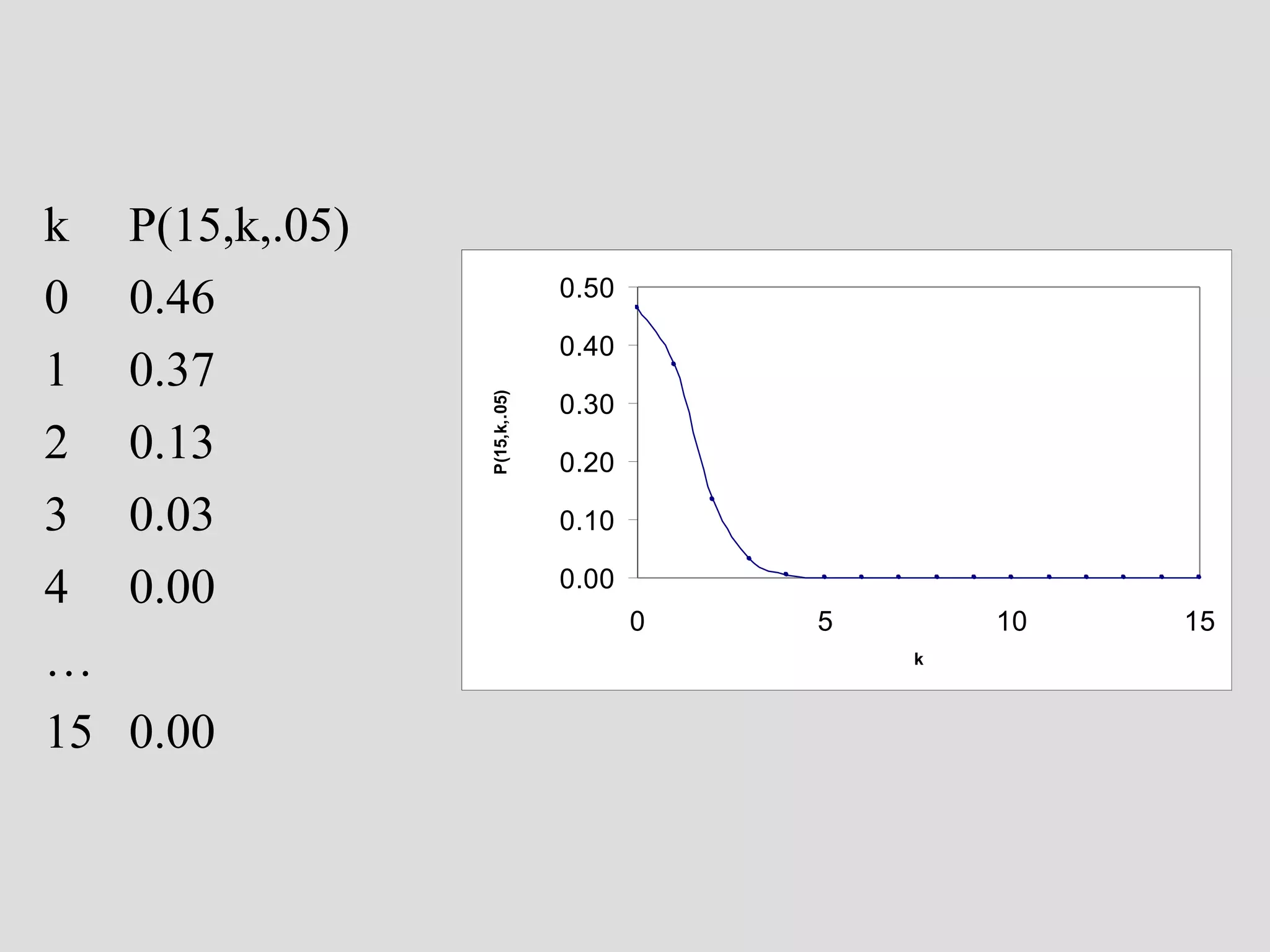
![• reverse the logic: assume that it is a ceramic
workshop
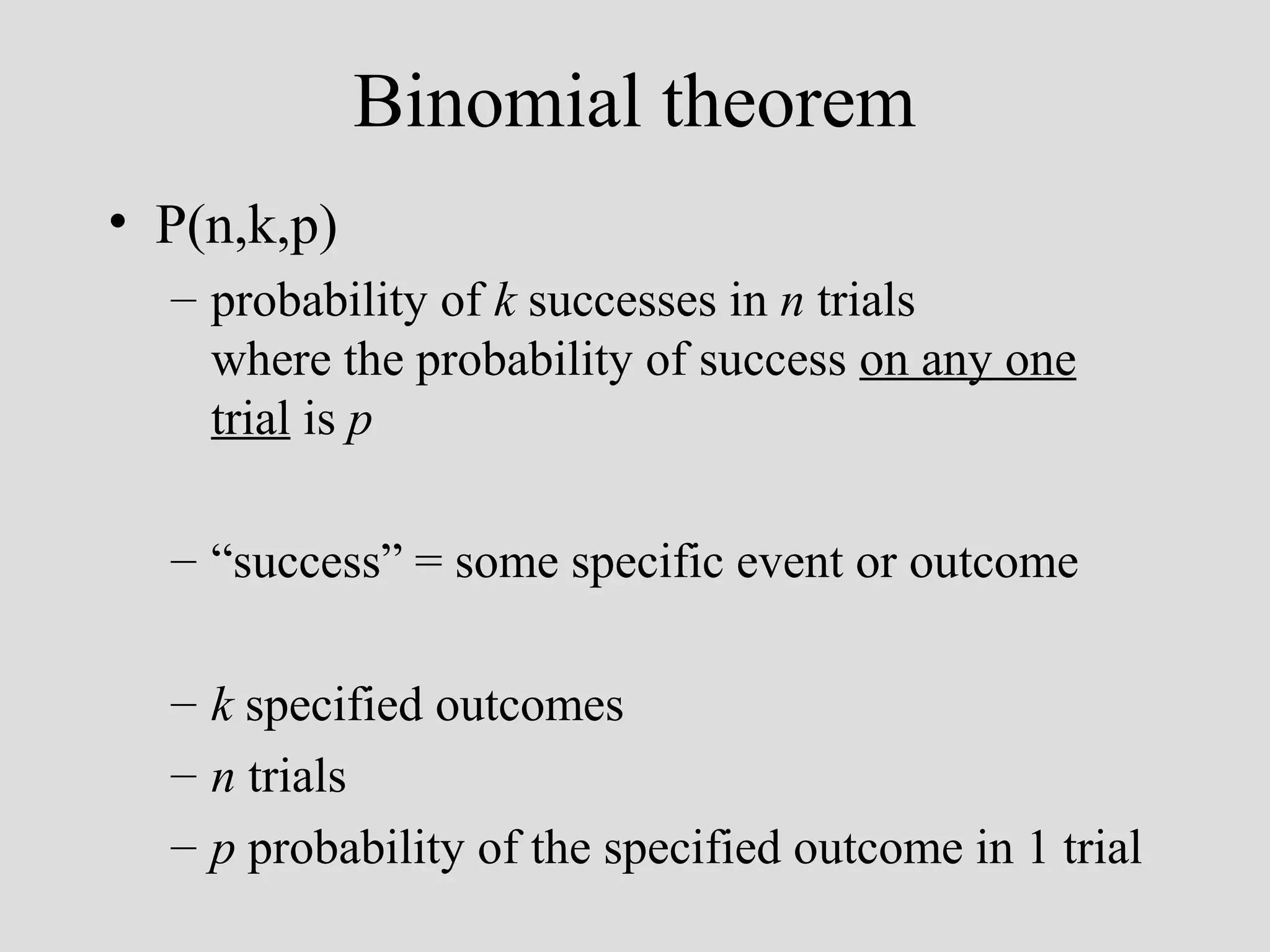
• new question:
– how likely is it to have missed collecting wasters in a
sample of 15 sherds from a real ceramic workshop??
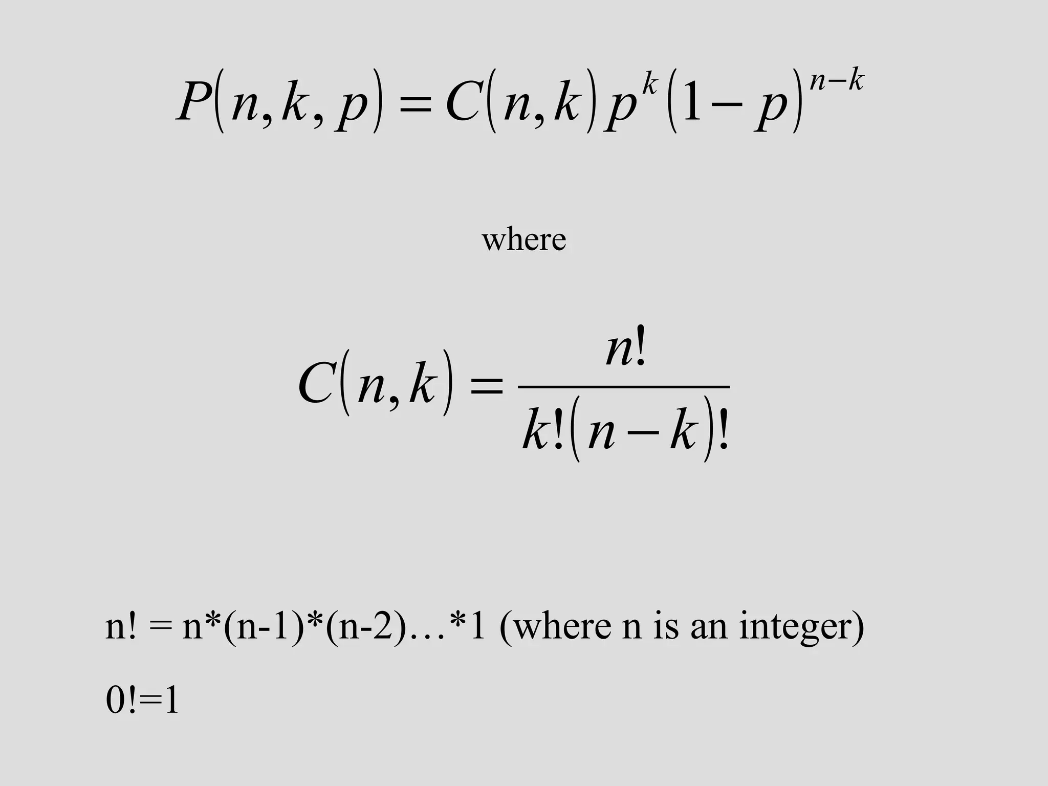
• P(n,k,p)
[n trials, k successes, p prob. of success on 1 trial]
• P(15,0,.05)
[we may want to look at other values of k…]](https://image.slidesharecdn.com/4probability-131209111956-phpapp02/75/4-probability-29-2048.jpg)


This document discusses key concepts in probability and how they can be applied in archaeology. It begins by explaining the frequentist and Bayesian approaches to probability. The basic concepts of probability, independent and conditional probability, and Bayes' Theorem are then defined. Examples are provided to demonstrate how binomial probability, probability density functions, and cumulative density functions can help archaeologists evaluate the significance of artifact samples and absence of types. Specifically, these statistical tools allow researchers to assess how likely it is their results are due to chance rather than reflecting real patterns in the archaeological record.


