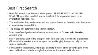
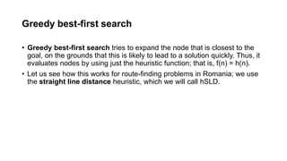
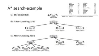
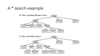
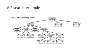
This document discusses various informed search algorithms including best-first search, greedy best-first search, A* search, and memory-bounded variants like IDA* and RBFS. It explains that A* search is optimal if the heuristic is admissible and consistent, and compares the performance of different heuristics for problems like the 8-puzzle. Memory-bounded algorithms trade optimality for practicality on large problems. Learning search control knowledge is also proposed.

1. Informed Search Algorithms
Dr. V. E. Sathish kumar
Dr.R.R.Rajalaxmi
Kongu Engineering College
Perundurai

2. Best First Search
• Best-first search is an instance of the general TREE-SEARCH or GRAPH-
SEARCH algorithm in which a node is selected for expansion based on an
evaluation function, f(n).
• The evaluation function is construed as a cost estimate, so the node with the lowest
evaluation is expanded first.
• The choice of f determines the search strategy.
• Most best-first algorithms include as a component of f a heuristic function,
denoted h(n):
• h(n) = estimated cost of the cheapest path from the state at node n to a goal state.
(Notice that h(n) takes a node as input, but, unlike g(n), it depends only on the
state at that node.)
• For example, in Romania, one might estimate the cost of the cheapest path from
Arad to Bucharest via the straight-line distance from Arad to Bucharest.

3. Greedy best-first search
• Greedy best-first search tries to expand the node that is closest to the
goal, on the grounds that this is likely to lead to a solution quickly. Thus, it
evaluates nodes by using just the heuristic function; that is, f(n) = h(n).
• Let us see how this works for route-finding problems in Romania; we use
the straight line distance heuristic, which we will call hSLD.

9. A* search
• evaluates nodes by combining g(n), the cost to reach the node, and h(n), the cost
to get from the node to the goal
f(n) = g(n) + h(n)
• Since g(n) gives the path cost from the start node to node n, and h(n) is the
estimated cost of the cheapest path from n to the goal, we have f(n) = estimated
cost of the cheapest solution through n
• reasonable thing to try first is the node with the lowest value of g(n) + h(n)
• A∗ search is both complete and optimal
• identical to UNIFORM-COST-SEARCH except that A∗ uses g + h instead of g

10. A* search-example

11. A * search-example

12. A * search-example

13. Conditions for optimality: Admissibility and
consistency
• admissible heuristic
• never overestimates the cost to reach the goal
• E.g-the straight-line distance hSLD that we used in getting to Bucharest
• Consistency
• required only for applications of A∗ to graph search
• A heuristic h(n) is consistent if, for every node n and every successor n of n
generated by any action a, the estimated cost of reaching the goal from n is
no greater than the step cost of getting to n plus the estimated cost of
reaching the goal from n’ :

14. Optimality of A*
• Properties
• tree-search version of A∗ is optimal if h(n) is admissible
• graph-search version is optimal if h(n) is consistent
• if h(n) is consistent, then the values of f(n) along any path are nondecreasing
• sequence of nodes expanded by A∗ using GRAPH-SEARCH is in nondecreasing order of
f(n)
• complexity of A∗ often makes it impractical to insist on finding an optimal solution.
• variants of A∗ can find suboptimal solutions quickly, or design heuristics that are more
accurate but not strictly admissible
• A∗ usually runs out of space long before it runs out of time
• A∗ is not practical for many large-scale problems

15. Memory-bounded heuristic search
• iterative-deepening A∗ (IDA∗)
• Cutoff used is the f-cost (g+h) rather than the depth
• IDA∗ is practical for many problems with unit step costs
• it suffers from the same difficulties with real valued costs as does the
iterative version of uniform-cost search

16. Recursive best-first search (RBFS)
• mimic the operation of standard best-first search, but using only linear space
• uses the f-limit variable to keep track of the f-value of the best alternative path
available from any ancestor of the current node
• If the current node exceeds this limit, the recursion unwinds back to the
alternative path
• As the recursion unwinds, RBFS replaces the f-value of each node along the path
with a backed-up value—the best f-value of its children
• RBFS remembers the f-value of the best leaf in the forgotten subtree and can
therefore decide whether it’s worth reexpanding the subtree at some later time
• IDA∗ and RBFS suffer from using too little memory

17. RBFS Stages
The path via Rimnicu Vilcea is followed until the current best leaf (Pitesti) has a value that is worse than the
best alternative path (Fagaras).

18. RBFS Stages
The recursion unwinds and the best leaf value of the forgotten subtree (417) is backed up to
Rimnicu Vilcea; then Fagaras is expanded, revealing a best leaf value of 450.

19. RBFS Stages
The recursion unwinds and the best leaf value of the forgotten subtree (450) is backed up to Fagaras; then Rimnicu Vilcea is
expanded. This time, because the best alternative path (through Timisoara) costs at least 447, the expansion continues to
Bucharest

20. RBFS
• RBFS retains more information in memory, but it uses only linear space:
even if more memory were available
• Two algorithms that use available memory are MA∗ (memory-bounded A∗)
and MA* SMA∗ (simplified MA∗).
• SMA∗
• it cannot add a new node to the search tree without dropping an old
one
• always drops the worst leaf node—the one with the highest f-value
• backs up the value of the forgotten node to its parent
• regenerates the subtree only when all other paths have been shown to
look worse than the path it has forgotten

21. Learning to search better
• Could an agent learn how to search better?
• metalevel state space
• Each state in a metalevel state space captures the internal (computational)
state of a program that is searching in an object-level state space
• Each state in a metalevel state space captures the internal
(computational) state of a program that is searching in an object-level
state space
• Internal state of A*-current search tree

22. HEURISTIC FUNCTIONS
• 8-puzzle problem
• h1 = the number of misplaced tiles.
• all of the eight tiles are out of position, so the start state would have h1 = 8. h1 is an
admissible heuristic because it is clear that any tile that is out of place must be moved at
least once.
• h2 = the sum of the distances of the tiles from their goal positions.
• Because tiles cannot move along diagonals, the distance we will count is the sum of the
horizontal and vertical distances. This is sometimes called the city block distance or
Manhattan distance.
• h2 is also admissible because all any move can do is move one tile one step closer to the goal.
• Tiles 1 to 8 in the start state give a Manhattan distance of
h2 = 3+1 + 2 + 2+ 2 + 3+ 3 + 2 = 18

23. Effect of heuristic accuracy on performance
Effective branching factor
• If the total number of nodes generated by A∗ for a particular problem is N and the solution depth is d, then b∗ is the
branching factor that a uniform tree of depth d would have to have in order to contain N + 1 nodes

24. References
1. Stuart Russell and Peter Norvig, "Artificial Intelligence: A Modern Approach", 3rd
Edition, Pearson Education, NA, 2013.
2. Elaine Rich, Kelvin Knight and Shivashankar B Nair, "Artificial Intelligence", 3rd
Edition, McGraw Hill Education Private Limited, India, 2017.