3645754 content

Journal of Economics and Sustainable Development www.iiste.org
ISSN 2222-1700 (Paper) ISSN 2222-2855 (Online)
Vol.2, No.6, 2011

Supply Response of Rice in Ghana: A Co-integration Analysis
John K.M. Kuwornu (Corresponding author)
Department of Agricultural Economics and Agribusiness, P. O. Box LG 68,
University of Ghana, Legon-Accra, Ghana
Tel: +233 245 131 807 E-mail: jkuwornu@ug.edu.gh / jkuwornu@gmail.com
Maanikuu P. M. Izideen
Tel: +233 241 913 985 E-mail: maanikuu@yahoo.com
Yaw B. Osei-Asare
Tel: +233 209 543 766 E-mail: yosei@ug.edu.gh

Received: October 1st, 2011
Accepted: October 11th, 2011
Published: October 30th, 2011

Abstract
This study presents an analysis of the responsiveness of rice production in Ghana over the period
1970-2008. Annual time series data of aggregate output, total land area cultivated, yield, real prices of rice
and maize, and rainfall were used for the analysis. The Augmented-Dickey Fuller test was used to test the
stationarity of the individual series, and Johansen maximum likelihood criterion was used to estimate the
short-run and long-run elasticities. The land area cultivated of rice was significantly dependent on output,
rainfall, real price of maize and real price of rice. The elasticity of lagged output (12.8) in the short run was
significant at 1%, but the long run elasticity (4.6) was not significant. Rainfall had an elasticity of 0.004 and
significant at 10%. Real price of maize had negative coefficient of -0.011 and significant at 10%
significance level. This is consistent with theory since a rise in maize price will pull resources away from
rice production into maize production. The real price of rice had an elasticity of 2.01 and significant at 5%
in the short run and an elasticity of 3.11 in the long run. The error correction term had the expected negative
coefficient of -0.434 which is significant at 1%. It was found that in the long run only real prices of maize
and rice were significant with elasticities of -0.46 and 3.11 respectively. The empirical results also revealed
that the aggregate output of rice in the short run was found to be dependent on the acreage cultivated, the
real prices of rice, rainfall and previous output with elasticities of 0.018, 0.01, 0.003 and 0.52 respectively.
Real price of rice and area cultivated are significant 10% level of significance while rainfall and lagged
output are significant 5%. In the long run aggregate output was found to be dependent on acreage cultivated,
real price of rice, and real price maize with elasticities of 0.218, 0.242 and -0.01 respectively at the 1%
significance level. The analysis showed that short-run responses in rice production are lower than long-run
response as indicated by the higher long-run elasticities. These results have Agricultural policy implications
for Ghana.

Key Words: Supply response, Rice, Error Correction Model, Co-integration Analysis, Ghana

1. Introduction
One of the most influential policy prescriptions for low-income countries ever given by development
economists has been to foster industrialization by withdrawing resources from agriculture (e.g., Lewis,
1954). There is robust evidence that the majority of policy makers followed this prescription at least until
the mid-1980s. The results of a comprehensive World Bank study (Krueger et al., 1992), for example, show
for the period 1960 –1985 that in most countries examined, agriculture was taxed both directly via

1

Vol.2, No.6, 2011

interventions in agricultural markets and indirectly via overvalued exchange rates and import substitution
policies. It is not obvious whether the disincentives for agricultural production have continued to exist since
the mid-1980s. On the one hand, most developing countries have adopted structural adjustment programs
which explicitly aim at a removal of the direct and indirect discrimination against agriculture. But, on the
other hand, it is known that many of these programs were not fully implemented, especially in Sub-Saharan
Africa (Kherallah et al., 2000; Thiele and Wiebelt 2000; World Bank, 1997). Hence it can be concluded that
a certain degree of discrimination still prevails.
One of the most important issues in agricultural development economics is supply response of crops. This
is because the responsiveness of farmers to economic incentives determines agricultures’ contribution to the
economy especially where the sector is the largest employer of the labour force. This is often the case in
third world low income countries. Agricultural pricing policy plays a key role in increasing farm production.
Supply response is fundamental to an understanding of this price mechanism (Nerlove and Bachman,
1960).
There is a notion that farmers in less developed countries respond slowly to economic incentives such as
price and income. Reasons cited for poor response vary from factors such as constraints on irrigation and
infrastructure to a lack of complementary agricultural policies. The importance of non-price factors drew
adequate attention in the literature: rainfall, irrigation, market access for both inputs and output, and literacy.
The reason cited for a low response to prices in less developed economies is the limited access to input and
product markets or high transaction costs associated with their use. Limited market access may be either
due to physical constraints such as absence of proper road links or the distances involved between the roads
and the markets, or institutional constraints like the presence of intermediaries (Mythili, 2008).
In Ghana, the goals of agricultural price policy are among others fair incomes for farmers, low food prices
for urban consumers, cheap raw materials for manufacturing (Ministry of Food and Agriculture (MOFA),
2005). Price support was one policy that was used by government in targeting these goals. Price support has
been used in many countries across the world. The prices of major commodities have been set below world
prices using subsidies and trade barriers, guaranteed prices (act as floors) and domestic market forces
determining actual prices (Food and Agriculture Organization (FAO), 1996). The effect of liberalization on
the growth of agriculture crucially depends on how the farmers respond to various price incentives.
For many low-income countries, the impact of structural reforms on economic growth and poverty
alleviation crucially depends on the response of aggregate agricultural supply to changing incentives.
Despite its policy relevance, the size of this parameter is still largely unknown (Thiele, 2000).
Rice is a very important crop especially for those areas where it is produced. Rice is gradually taking the
position as the main staple food for the majority of families in Ghana especially in the urban centres. The
growth in consumption of rice has been not been matched with a corresponding growth in local production
of the crop. Per capita consumption of rice has steadily increased over the years since the 1980s from about
12.4kg/person /year in 1984 to about 20kg/person /year (Statistical Research and Information Division
(SRID), 2005). It continued to rise to 38kg/person/year in 2008 (National Rice Development Policy
(NRDP), 2009). Over the last decade rice per capita consumption has increased by more than 35%. This is
attributed mainly to the rapid urbanization and changes in food consumption patterns. It is estimated based
on population and demand growth rates that per capita consumption will reach 41.1kg by 2010 and 63.0kg
by 2015 giving an aggregate demand of 1,680,000tons/year (Statistical Research and Information Division
(SRID), 2005). Changes in population dynamics and the taste or preference for foreign products is
contributing to this trend. These changes are significant considering the rate of population growth. Ghana’s
population has grown by about 70% from 12.3 million in 1984 to about 21 million in 2004. The population
is now 24 million (Ghana Statistical Service (GSS), 2011).
The growing quantum of rice imports into the country has also been triggered partly by the fall in world
market price. This is largely due to increased output levels in India and South Asia. Massive subsidies in
rice exporting countries have also contributed to this phenomenon. Despite all these developments there
seem to be a lack of coherent and comprehensive national policy for rice in Ghana. From the period of
economic recovery and structural adjustment, the country has had to embark on trade liberalization and the
removal of all forms of subsidies on agriculture. These policies no doubt have adversely affected rice
production in the country. The smallholder rural farmer is faced with unfair competition from abroad. The
2

Vol.2, No.6, 2011

role of incentives to farmers has generally been sidelined or ignored in most developing countries due to
conditions of trade liberalization and global trade integration. However, a number of empirical studies in
other developing economies addressed the question of farmers’ response to economic incentives and
efficient allocation of resources (e.g. Chinyere, 2009). The agricultural sector in Ghana has undergone
various policy regimes which has affected both the factor and product market resulting in changes in the
structure of market incentives (prices) faced by farmers. Most of these policies have, however, not been
crop specific and therefore has wide variations in the quantum of changes in the incentives. This study
therefore follows the supply response framework of analysis to examine the dynamics of the supply of rice
in Ghana. Effort in this direction will have to be preceded by a thorough analysis of the factors that affects
the supply of rice. These teething problems lead to the following research questions;
How responsive is rice production to price and non-price factors? What are the long run and short run
elasticities of rice production? What are the trends in area cultivated, output and real prices of output?
Therefore, objective of the study is threefold: (a) Examine the acreage and output response of rice
production in Ghana. (b) Estimate and compare the long run and short run elasticities of rice production.
(c) Analyze the trends in output, area cultivated and real prices.
The rest of the paper is structured as follows. Section 2 outlines the methodology. In section 3 we present
the empirical applications and the results. Section 4 provides the conclusions.

2.0 Methodology
This section presents the methodology of the study.
2.1 Linear Regression
Linear regression was conducted to determine the growth rates of the variables over the study period. Time
in years was regressed on acreage cultivated, aggregate output, real price of rice separately.
2.2 Time series analysis
In empirical analysis using time series data it is important that the presence or absence of unit root is
established. This is because contemporary econometrics has indicated that regression analysis using time
series data with unit root produce spurious or invalid regression results (e.g. Townsend, 2001). Most time
series are trended over time and regressions between trended series may produce significant parameters
with high R2s, but may be spurious or meaningless (Granger and Newbold, 1974). When using the classical
statistical inference to analyze time series data, the results are only stationary when the series are stationary.
The solution to this problem was initially provided by Box and Jenkins (1976), by formulating regressions
in which the variables were expressed in first difference. Their approach simply assumed that
non-stationary data can be made stationary by repeated differencing until stationarity is achieved and then
to perform the regression using these differenced variables. However, according to Davidson et al., (1978),
this process of repeated differencing even though leads to stationarity of the series; it is achieved at the
expense of losing valuable long run information. This posed a new challenge to time series econometrics.
The concept of cointegration was introduced to solve these problems (Granger, 1981; Engle and Granger,
1987). By using the method of cointegration an equation can be specified in which all terms are stationary
and so allow the use of classical statistical inference. It also retains information about the long run
relationship between the levels of variables, which is captured in the stationary co-integrating vector. This
vector will comprise the parameters of the long run equilibrium and corresponds to the parameters of the
error correction term in the second stage regression (Mohammed, 2005). The cointegration approach takes
into consideration the long-run information such that spurious results are avoided.

2.3 Stationarity Tests

A data series is said to be stationary if it has a constant mean and variance. That is the series fluctuates around
its mean value within a finite range and does not show any distinct trend over time. In a stationary series
displacement over time does not alter the characteristics of a series in the sense that the probability
distribution remains constant over time. A stationary series is thus a series in which the mean, variance and
covariance remain constant over time or in other words do not change or fluctuate over time. In a stationary

3

Vol.2, No.6, 2011

series the mean always has the tendency to return to its mean value and to fluctuate around it in a more or less
constant range, while a non-stationary series has a changing mean at different points in time and its variance
change with the sample size (Mohammed, 2005). The conditions of stationarity can be illustrated by the
following:

Yt = ѳYt-1 + µ t t=1………T (1)
Where µ t is a random walk with mean zero and constant variance. If ѳ < 1, the series Yt stationary and if
ѳ = 1 then the series Yt is non-stationary and is known as random walk. In other words the mean, variance
and covariance of the series Yt changes with time or have an infinite range. However Yt can be made
stationary by differencing. Differencing can be done multiple times on a series depending on the number of
unit roots a series has. If a series becomes stationary after differencing d times, then the series contains d
unit roots and hence integrated of order d denoted as I (d). Thus, in equation (1) where ѳ = 1, Yt has a unit
root. A stationary series could also exhibit other properties such as when there are different kinds of time
trends in the variable.
The DF (Dickey-Fuller)-statistic used in testing for unit root is based on the assumption that µ t is white
noise. If this assumption does not hold, it leads to autocorrelation in the residuals of the OLS regressions
and this can make invalid the use of the DF-statistic for testing unit root. There are two approaches to solve
this problem (Towsend, 2001). In the first instance the equations to be tested can be generalized. Secondly
the DF-statistics can be adjusted. The most commonly used is the first approach which is the Augmented
Dickey-Fuller (ADF) test. µ t is made white noise by adding lagged values of the dependent variable to the
equations being tested, thus:
∆Yt = (ѳ1 – 1) Yt-1 + IYt-I + µ t (2)
∆Yt = α2 + (ѳ2 – 1) Yt-1 + I ∆Yt-I + µ t (3)
∆Yt= α3+β3t(ѳ3–1)Yt-1+ I ∆Yt-I + µ t (4)
The ADF test uses the same critical values with DF. The results of the ADF test for unit roots for each of
the data series used in this study are presented in in the next section using equation (4) where Yt is the
series under investigation, t is the time trend, α3 is the constant term and µ t are white noise residuals.
Eviews was used in the analysis, all the data series was tested for stationarity and the results are presented
in section three.
2.4 Cointegration
Cointegration is founded on the principle of identifying equilibrium or long run relationships between
variables. If two data series have a long run equilibrium relationship it implies their divergence from the
equilibrium are bounded, that is they move together and are cointegrated. Generally for two or more series
to be co-integrated two conditions have to be met. One is that the series must all be integrated to the same
order and secondly a linear combination of the variables exist which is integrated to an order lower than
that of the individual series. If in a regression equation the variables become stationary after first
differencing, that is I (1), then the error term from the cointegration regression is stationary, I (0)
(Hansen and Juselius, 1995). If the cointegration regression is presented as:
Yt = α + βXt + µ t (5)
where Yt and Xt are both I (1) and the error term is I (0), then the series are co-integrated of order I (1,0 )
and β measures the equilibrium relationship between the series Yt and Xt and µ t is the deviation from the
long-run equilibrium path. An equilibrium relationship between the variables implies that even though Yt
and Xt series may have trends, or cyclical seasonal variations, the movement in one are matched by
movements in the other. The concept of cointegration has implications for economists. The economic
interpretation that is accepted is that if in the long-run two or more series Yt and Xt themselves are
non-stationary, they will move together closely over time and the difference between them is constant
(stationary) (Mohammed 2005).
2.4.1 Testing for Cointegration
There are two most commonly used methods for testing cointegration. The Augmented Dickey-Fuller
residual based test by Engle and Granger (1987), and the Johansen Full Information Maximum Likelihood
(FIML) test (Johansen and Juselius, 1990). For the purpose of this study the Johansen Full Information
Maximum Likelihood test is used due to its advantages. The major disadvantage of the residual based test is
4

Vol.2, No.6, 2011

that it assumes a single co-integrating vector. But if the regression has more than one co-integrating vector
this method becomes inappropriate (Johansen and Juselius, 1990). The Johansen method allows for all
possible co-integrating relationships and allows the number of co-integrating vectors to be determined
empirically.
2.4.2 Johansen Full Information Maximum Likelihood Approach
The Johansen approach is based on the following Vector Autoregression
Zt = AtZt-1 + … + AkZt-k + µ t (6)
Where Zt is an (n×1) vector of I(1) variables (containing both endogenous and exogenous variables), At is
(n×n) matrix of parameters and µ t is (n×1) vector of white noise errors. Zt is assumed to be nonstationary
hence equation (6) can be rewritten in first difference or error correction form as;
∆Zt = Γ1∆Zt-1 + … + Γk-1∆Zt-k+1 + πZt-k + µ t (7)

where Γ1 = - ( 1- A1 - A2 - … -Ai), (i = 1, …, k-1) and π = - (1- A1-A2- …-Ak).
Γ1 gives the short run estimates while π gives the long run estimates. Information on the number of
co-integrating relationships among variables in Zt is given by the rank of the matrix π. If the rank of π
matrix r, is 0 < r > n, there are r linear combinations of the variables in Zt that are stationary. Thus π can be
decomposed into two matrices α and β where α is the error correction term and measures the speed of
adjustment in ∆Zt and β contains r co-integrating vectors, that is the cointegration relationship between
non-stationary variables. If there are variables which are I(0) and are significant in the long run
co-integrating space but affect the short run model then equation (7) can be rewritten as:
∆Zt = Γ1∆Zt-1 + πZt-k + vDt + µ t (8)
where Dt represents the I(0) variables.
To test for co-integrating vector two likelihood ratio (LR) tests are used. The first is the trace test statistic;

Λtrace = -2lnQ = -T i) (9)
Which test the null hypothesis of r co-integrating vectors against the alternative that it is greater than r. The
second test is known as the maximal-eigen value test:
Λmax = -2 ln(Q: r 1 r + 1 = -T ln(1-λr+1 ) (10)
which test the null hypothesis of r co-integrating vectors against the alternative of r+1 co-integrating
vectors. The trace test shows more robustness to both skewness and excess kurtosis in the residuals than the
maximal eigen value test (Harris, 1995). The error correction formulation in (7) includes both the difference
and level of the series hence there is no loss of long run relationship between variables which is a
characteristic feature of error correction modeling.
It should be noted that in using this method, the endogenous variables included in the Vector
Autoregression (VAR) are all I(1), also the additional exogenous variables which explain the short run
effect are I(0). The choice of lag length is also important and the Akaike Information Criterion (AIC), the
Scharz Bayesian Criterion (SBC) and the Hannan-Quin Information Criterion (HQ) are used for the
selection.
According to Hall (1991) since the process might be sensitive to lag length, different lag orders should be
used starting from an arbitrary high order. The correct order is where a restriction on the lag length is
rejected and the results are consistent with theory.
2.5 Error Correction Models (ECMs)
The idea behind the mechanism of error correction is that a proportion of disequilibrium from one period is
corrected in the next period in an economic system (Engle and Granger, 1987). The process of making a
data series stationary is either done by differencing or inclusion of a trend. A series that is made stationary
by including a trend is trend stationary and a series that is made stationary by differencing is difference
stationary. The process of transforming a data series into stationary series leads to loss of valuable long run
information (Engle and Granger, 1987). Error correction models helps to solve this problem.
The Granger representation theorem is the basis for the error correction model which indicates that if the
variables are cointegrated, there is a long-run relationship between them and can be described by the error
correction model. The following equation shows an ECM of agricultural supply response involving the
variables Y and X in its simplest form:
5

Vol.2, No.6, 2011

∆Yt = α∆Xt – ѳ(Yt-1 – γXt-1)+µ t (11)
Where µ t is the disturbance term with zero mean, constant variance and zero covariance. Parameter α takes
into account the short run effect on Y of the changes in X, while γ measures the long-run equilibrium
relationship between Y and X that is:
Yt = γXt + µ t (12)
Where Yt-1 – γYt-1 + µ t-1 measures the divergence (errors) from long-run equilibrium. Also ѳ measures the
extent of error correction by adjustment in Y and its negative sign indicates that the adjustment is in the
direction which restores the long-run relationship (Hallam and Zanoli, 1993). In order to estimate equation
(5), Engle and Granger (1987) proposed a two stage process. Firstly the static long run cointegration
regression (6) is estimated to test cointegration between the two variables. If cointegration exists the lagged
residuals from equation (5) are used as error correction term in the Error Correction Model (in equation 6)
to estimate the short run equilibrium relationship between the variables in the second stage. The validity of
the Error Correction Models (ECMs) depends upon the existence of a long-run or equilibrium relationship
among the variables (Mohammed, 2005).
The Error Correction Model (ECM) has several advantages. It contains a well-behaved error term and
avoids the problem of autocorrelation. It allows consistent estimation of the parameters by incorporating
both short-run and long-run effects. Most importantly all terms in the ECM are stationary. It ensures that no
information on the levels of the variables is lost or ignored by the inclusion of the disequilibrium terms
(Mohammed, 2005). ECM solves the problems of spurious correlation because ECMs are formulated in
terms of first difference which eliminates trends from the variables (Ganger and Newbold, 1974). It avoids
the unrealistic assumption of fixed supply based on stationary expectations in the partial adjustment model.
2.6 Supply Response Models
This study estimated the total area cultivated and aggregate output of rice in Ghana using double
logarithmic regression models.
Area cultivated of rice (lgarea) is a function of own price (Lrp), rainfall (lgrain), aggregate output (lgoutput)
and price of maize (lmp). The equation used for the regression is:
Lgarea = f1 (Lgoutput, Lrp, Lgrain, Lmp) (13)
Aggregate output of rice (lgoutput) is a function of the area cultivated (lgarea), the price of rice (Lrp), price
of maize (Lmp), rainfall (lgrain). The estimating equation is:
Lgoutput = f2 (lgrain, Lrp, Lmp, Lgarea)1. (14)

3. Empirical Application and Results
3.1 Results for linear regression
Table 1: The results of the regression analysis for the trend of the variables against time
Variable Coefficient Std error t-statistic R2 F-statistic Prob
Lgarea 1.334274 1.149167 1.61079 0.035154 0.253046 0.2530
Lgoutput -13.86625 68.09380 -0.20364 0.005889 0.844432 0.8444
lgyield -25.99348 35.51112 -0.73198 0.071100 0.487957 0.4880
Lrp 2.588941 5.221601 4.956136 0.399186 24.58311 0.0000

As can be seen from table 1 the results indicated that the regression for area, output and yield turned out
insignificant. Only the trend of real price of rice was significant at 1% significance level. Real rice price
yielded a positive coefficient of 2.589 which implies that for each year the real price of rice grew by 2.589
units.
3.2 Unit Root Test Results
As a requirement for cointegration analysis the data was tested for series stationarity and to determine the
order of integration of the individual variables. For cointegration analysis to be valid all series must be
integrated of the same order usually of order one (Towsend, 2001). Eviews was used to perform these tests.

1
Price of maize is included because we assume that the same resources (land type, fertilizer etc.) can be used to
produce both maize and rice. Hence, a rise in the price of maize will pull resources away from rice production to maize
production.
6

Vol.2, No.6, 2011

The data series on annual acreage cultivated (Lgarea), aggregate output (Lgoutput), aggregate yield
(Lgyield), real price of rice (Lrp), real price of maize (Lmp), rainfall (Lgrain) was tested for unit root for
the study period 1970 - 2008. The Augmented Dickey-Fuller test was used for this test. The results are
presented below.

Table 2: Results of unit root test at levels
Series ADF test Mackinnon Lag-length Prob Conclusion
statistic critical value
Lgarea 2.221125 3.615588 2 0.2024 Non-stationary
Lgoutput 1.519278 5.119808 2 0.4582 Non-stationary
Lgyield 0.103318 4.580648 2 0.9419 Non-stationary
Lmp 0.378290 3.621023 2 0.9026 Non-stationary
Lrp 1.429037 3.615588 2 0.5579 Non-stationary

Lgrain 3.006033 2.963972 7 0.0457 Stationary

The results of the unit root test after first differencing are presented in table 3.

Table 3: Results of unit root test at first differences
Series ADF test Mackinnon Lag-length Prob Conclusion
statistic critical value
Lgarea 7.517047 3.621023 2 0.0000 I(1)
Lgoutput 9.577098 3.621023 2 0.0000 I(1)
Lgyield 7.517047 3.621023 2 0.0000 I(1)
Lmp 10.02189 3.621023 2 0.0000 I(1)
Lrp 6.346392 3.626784 2 0.0000 I(1)

Note; All variables are in log form. The ADF method test the hypothesis that H0 : X ~ I(1), that is, has unit
root (non-stationary) against H1 : X ~ I(0), that is, no unit root (stationary). The Mackinnon critical values
for the rejection of the null hypothesis of unit root are all significant at 1%. Lgarea denotes log of area
cultivated, Lgoutput denotes log total output, Lgyield denotes log of yield, Lmp denotes log of maize price,
Lrp denotes log of rice price and Lgrain denotes log of rainfall.
The results of the unit root tests showed that all the series are non-stationary at levels except for rainfall
which is stationary at levels as shown in table 2 above. However as expected all the non-stationary series
became stationary after first differencing. From table 2 the null hypothesis of unit root could not be rejected
at levels since none except rainfall of the ADF test statistics was greater than the relevant Mackinnon
Critical values. Hence the null of the presence of unit root is accepted.
However the hypothesis of unit root in all series was rejected at 1% level of significance for all series after
first difference since the ADF test statistics are greater than the respective Mackinnon critical values as
shown in table 3 above.
3.3 Cointegration Results
When the order of integration of the data series have been established, the next step in the process of
analysis is to determine the existence or otherwise of cointegration in the series. This is to establish the
existence of valid long-run relationships between variables. Basically there are two most commonly used
methods to test for cointegration. These were suggested by Engle and Granger (1987) and Johansen and
Juselius (1990). This study applies the Johansen approach which provides likelihood ratio tests for the
presence of number of co-integrating vectors among the series and produces long-run elasticities. The Error
correction model was then used to estimate short-run elasticities.
7

Vol.2, No.6, 2011

3.3.1 Supply Response of Rice Output
Firstly, the Vector Error Correction Modeling (VECM) procedure using the Johansen method involves
defining an unrestricted Vector Autoregression (VAR) using the following equation.
Zt=AtZt-1+…+AkZt-1+µ t (15)
Likelihood Ratio (LR) tests were conducted with maximum of three lags due to the short time series. The
results are shown in table 4.

Table 4: Results for lag selection output model
VAR Lag Order Selection Criteria
Endogenous variables: OUTPUT AREA MP RP
Exogenous variables: C RAIN

Lag LogL LR FPE AIC SC HQ

0 -1208.968 NA 6.64e+32 86.92626 87.30689* 87.04262
1 -1184.928 37.77692 3.84e+32 86.35198 87.49387 86.70107
2 -1174.563 13.32579 6.37e+32 86.75452 88.65766 87.33633
3 -1138.068 36.49514* 1.92e+32* 85.29058* 87.95499 86.10511*

* indicates lag order selected by the criterion
LR: sequential modified LR test statistic (each test at 5% level)
FPE: Final prediction error
AIC: Akaike information criterion
SC: Schwarz information criterion
HQ: Hannan-Quinn information criterion
LogL: Log-likelihood

The results indicate that the Akaike Information Criterion (AIC) and the Hannan-Quin information criterion
(HQ) selected lag order three while the Scharz Bayesian Criterion (SBC) selected the lag order zero. Thus,
this study selects the lag order three as the order for the VAR models. The next step in the Johansen method
is to test for the number of co-integrating vectors among the series in the model.
The results for the cointegration test imply that both the trace test and the maximum eigen value test selects
the presence of one co-integrating vector, thus it can be concluded that the variables in the model are
co-integrated. The Johansen model is a form of Error Correction Model. When only one co-integrating
vector is established its parameters can be interpreted as estimates of long run co-integrating relationship
between the variables (Hallam and Zanoli, 1993). This implies that the estimated parameter values from
this equation when normalized on output are the long run elasticities for the model. Eviews automatically
produces the normalized estimates. These coefficients represent estimates of long-run elasticities with
respect to area cultivated, real price of rice and real price of maize. The normalized cointegration equation
for rice output is given below;
Output=0.216748area+0.241522rp-0.009975mp-12841.69 (16)
Since cointegration has been established among the variables, then the dynamic ECM can be used for
supply response analysis since it provides information about the speed of adjustment to long run
equilibrium and avoids the spurious regression problem between the variables (Engle and Granger, 1987).
The ECM for rice output is presented as;
∆output = α0+ 1i∆outputt-i + 2i∆areat-i + 3i∆rpt-I + 4i∆mpt-I + 5rain – θECt-I (17)
Where θECt-I = α (β1outputt-I – β2areat-I – β3rpt-I – β4mpt-I)
8

Vol.2, No.6, 2011

In the ECM model above, the α’s explain the short run effect of changes in the explanatory variables on the
dependent variable whereas β’s represent the long run equilibrium effect. θECt-I is the error correction term
and correspond to the residuals of the long run cointegration relationship, that is the normalized equation
(16). The negative sign on the error correction term indicates that adjustments are made towards restoring
long run equilibrium. This representation ensures that short run adjustments are guided by and consistent
with the long run equilibrium relationship. This method provides estimates for the short run elasticities, that
is the coefficients of the difference terms and, whereas the parameters from the Johansen cointegration
regression are estimates of the long run elasticities (Townsend and Thirtle, 1994). In selecting the best ECM
estimates, models with lag lengths are estimated and those with insignificant parameters are eliminated.
Note that the estimates presented above represent the short run effect of the explanatory variables on the
dependent variable. The long run effect is captured by the estimates of the normalised Johansen regression
results presented in equation (16). The diagnostic tests are the t-ratio test of the coefficients, LM test for
autocorrelation and the Jarque Berra test for normality of residuals.
Table 5: ECM results for rice output
Variable Coefficient t-statistic Prob

∆lgarea 0.017611 0.668907 0.0510

∆lgoutput(-1) 0.523393 2.283959 0.0319

lgRain 0.003740 0.997918 0.0328

∆lgmp -0.001107 -0.298174 0.7683

∆lgrp 0.009922 0.307758 0.0761

Residual -0.174253 -1.321005 0.0043

R2 (0.754242) F-statistic (2.523411) Prob(F-stat) 0.058261

It indicates that aggregate rice output is dependent on area cultivated, previous year’s output, and previous
year’s price of rice. The coefficient of maize price was not significant.
An R2 of 0.754 indicates that 75% of the variation in the dependent variable can be accounted for by
variation in the explanatory variables. The results indicate that area cultivated was significant at 10%, with
elasticity of 0.0176, which implies that a one percent increase in area cultivated of rice will lead to a
0.018 % increase in output in the short run. This is rather on the low side. This can be attributed to the fact
that an increase in the land cultivated without a necessary increase in the resources of the farmer will
increase adverse effect on the minimal resources available to the farmer hence resulting in this marginal
increase in output. This result also indicates that the productivity of the farmer reduces with increase in
farm size. The long run elasticity of area cultivated is 0.2167 (in equation (16)) is higher than the 0.0176 for
the short run. This indicates that over the long run farmers adjust their farm sizes more to output than in the
short run. That is, a 1% increase in area cultivated will lead to 0.217% increase in output in the long run.
Lagged output has elasticity of 0.523393 in the short run and is significant at the 5% significance level
implying that a one percent increase in output in a year will lead to a 0.52% increase in output the
subsequent year. This simply means that an increase in output will make capital available for the farmer to
invest in the subsequent year’s rice production activities. This is only true if the additional resource is
invested into the following year’s rice production activities.
Rainfall is significant at 5%. An elasticity of 0.003740 for rainfall indicates that a 1% increase in rainfall
will result in a 0.004% rise in output. This low impact of rainfall can be explained by the fact that a large
proportion of total rice output is produced under the irrigation projects across the country. This makes the
response of output to rainfall highly inelastic.
A coefficient of 0.009922 which is significant at 10% for real price of rice indicates that a 1% rise in real
9

Vol.2, No.6, 2011

prices will lead to 0.01% increase in output the subsequent year in the short run. This makes prices also
inelastic. This low rice price elasticity suggests that farmers do not always necessarily benefit from
increasing prices due to the structure of the marketing system. Middlemen and other marketing channel
members purchase the rice from farmers at the farm gate and thereafter transport it to market centres to be
sold. Hence when there is a rise in prices a little fraction of it is transmitted to the famer. The low price
elasticity could also be attributed to the fact that farmers are hindered by an array of constraints such as
land tenure issues, rainfall variability, lack of capital resources and credit facilities which limits their
capacity to respond to price incentives. The long run coefficient of 0.2415 indicates that 1% percent
increase in real prices will lead to a 0.24% increase in output. The long run elasticity far exceeds the short
run. This is because over the long run when prices show a continual rise, farmers are able to accumulate
capital enough to enhance production.
The residual which is the error correction term is significant at 1% and has the expected negative sign. It
measures the adjustment to equilibrium. Its coefficient of -0.174 indicates that the 17.4% deviation of rice
output from long run equilibrium is corrected for in the current period. This slow adjustment can be
attributed to the fact that famers in the short run are constrained by technical factors as mentioned earlier
which limits their ability to adjust immediately to price incentives.
In the long run maize price is significant at 1%. With a negative coefficient of 0.009975 it implies that a 1%
increase in the price of maize will lead to 0.01% reduction in the output of rice. This is to say that resources
will be diverted to maize production relative to rice production leading to the fall in rice output. However,
Maize price was not significant in the short run. The results of the LM test of serial correlation for up to
fifth order show that there is no serial correlation in the data set.
3.3.2 Supply Response of Area Cultivated
Testing for the selection of lag length yielded the same results for both the acreage and output models.
Hence the same lag order three is therefore used for the Vector Error Correction model (VEC).
The trace test selects one co-integrating vector while the eigen value test selects two co-integrating vectors.
But since the trace test is the more powerful test (Mohammed, 2005), the result from the trace test is used
here. Thus the acreage model has one co-integrating vector. The normalised cointegration equation for area
cultivated is given as;
lgarea =4.613649lgoutput+3.11429lrp–0.46020lmp–59247 (18)
The ECM for area cultivated is presented as;
∆lgarea = α0 + 1i ∆lgoutputt-i + 2i ∆lgareat-i + 3i ∆lgrpt-I + 4i ∆lgmpt-I + 5l lgrain –
θECt-I (19)
Where θECt-I = α (β1areat-I – β2outputt-I – β3rpt-I – β4mpt-I)

The result of the estimated ECM is given in table 6 below.
Table 6: ECM results for area cultivated
Variable Coefficient t-statistic Prob
∆lgarea(-1) 0.169747 1.343021 0.1192
∆lgoutput(-1) 12.80810 1.816372 0.0824
lgRain 0.003984 0.138622 0.0891
∆lmp(-1) -0.011350 -0.401819 0.0691
∆lrp(-1) 2.016747 1.440683 0.0265
Residual -0.435411 -1.043641 0.0047
R2 (0.770669) F-statistic Prob(F-stat) 0.017301
(1.707148)

An R2 of 0.77067 indicates that 77% 0f the variation in the dependent variable is accounted for by variation
in the explanatory variables. Output is significant at 10% with an elasticity of 12.80 indicating that a 1%
increase in output this year will increase land cultivated in the subsequent year by 12.8% in the short run.
Thus acreage cultivated is highly elastic with respect to output. An increase output level gives the farmers
an opportunity to acquire necessary resources and equipment to put more land under cultivation. Output
10

Vol.2, No.6, 2011

elasticity is even higher than that for real prices. This can be attributed to the fact that a large proportion of
output is for household consumption and thus is independent of prices. Increased output alone is enough
motivation to increase acreage under cultivation. In the long run output is insignificant. This because in the
long run land will get exhausted and output will be dependent on productivity (and not the area of land
cultivated).
Rainfall is significant at 10% with a coefficient of 0.003984; this implies a 1% increase in rainfall leads to
0.004% increase in area cultivated. This low response to rain can be attributed to the fact that large areas
under rice cultivation are in irrigated fields which depends less on rainfall for cultivation. Rainfall is an
exogenous variable (I(0)), hence it measures short run effect.
Maize price is significant at 10% with a negative coefficient of -0.011350 in the short run and -0.460 in the
long run. This means over the long run if maize prices are continually increasing farmers will commit more
resources into maize farming relative to rice farming. Thus as the price of maize rises area under rice
cultivation reduces both in the short and long run. In the short run a 1% increase in maize price reduces area
cultivated of rice by 0.0114% and by 0.46% in the long run.
Real price of rice was significant at 5% with elasticities of 2.017 and 3.11 in the short run and long run
respectively, thus price is elastic. This implies a 1% percent increase in real price of rice will result 2.017%
and 3.11% increase in acreage cultivated in the short run and long run respectively. This is expected since
in the long run farmers are able to adjust to overcome some the major challenges of production and hence
are able to adjust more to price incentives.
The error correction term has the expected negative sign and with a coefficient of 0.4354 indicating that
43.54% of the deviation from long run equilibrium is corrected for in the current period.
The results of the test for serial correlation show that is no autocorrelation in the series. The Jarque-Berra
test statistic of 10.18 with probability value of 0.25 implies that the residuals are normally distributed.
4. Conclusions
Economic theory in the past had been based on the assumption that time series data is stationary and hence
standard statistical techniques (Ordinary Least Squares regression (OLS)) designed for stationary series was
used. However, it is now known that many time series data are non-stationary and therefore using
traditional OLS methods will lead to invalid or spurious results. To address this problem, the method of
differencing was introduced. Differencing according to Granger however leads to loss of valuable long-run
information. Granger and Newbold (1974) introduced the technique of cointegration which takes into
account long-run information therefore avoiding spurious results while maintaining long-run information.
This study presents an analysis of the responsiveness of rice production in Ghana over the period
1970-2008. Annual time series data of aggregate output, total land area cultivated, yield, real prices of rice
and maize, and rainfall were used for the analysis.
The Augmented-Dickey Fuller test was used to test the stationarity of the individual series. The Johansen
maximum likelihood criterion is used to estimate the short-run and long-run elasticities.
The trend analysis for rice output, rice price, acreage cultivated, and yield revealed that only rice price is
significant at 1% significance level. The results imply that for each year, the price of rice will increase by
2.589 units.
All the time series data that was used were tested for unit root. They were found to be non-stationary at
levels but stationary after first differencing at the one percent significance level except for rainfall which
was stationary at levels at the 5% significance level. The Likelihood Ratio tests selection of lag order
selected order three by the AIC and HQ criteria for both models. The Johansen cointegration test selected
one cointegration vector (in both rice output and rice price models) indicating that the variables are
co-integrated. The diagnostic tests of serial correlation and normality test was done using the Lagrange
Multiplier test for autocorrelation and the Jarque-Berra test for normality of residuals. The results indicate
no serial correlation and normally distributed residuals.
The land area cultivated of rice was significantly dependent on output, rainfall, real price of maize and real
price of rice. The elasticity of lagged output was 12.8 in the short run and was significant at 1%. However,
this elasticity was not significant in the long run.
Rainfall had an elasticity of 0.004 and significant at 10%. Also real price of maize had negative coefficient
of -0.011 which was significant at 10%. This is consistent with theory since a rise in maize price will pull
11

Vol.2, No.6, 2011

resources away from rice production into maize production. The coefficient of the real price of maize
estimated by Chinere (2009) was -0.066 for rice farming in Nigeria. This is higher than the -0.011 estimated
for Ghana (in this study).
The real price of rice had an elasticity of 2.01 and significant at 5% in the short run and an elasticity of 3.11
in the long run. The error correction term had the expected negative coefficient of -0.434 which is
significant at 1%. It was found that in the long run only real prices of maize and rice were significant with
elasticities of -0.46 and 3.11 respectively. The error correction estimated by Chinere (2009) was -0.575.
This indicates that adjustment to long run equilibrium is faster in Nigeria. This could be attributed to better
agricultural infrastructure in Nigeria compared to Ghana. The error correction for Indian rice in the rice
zone as estimated by Mohammed (2005) was -0.415. This could be attributed to the fact that Indian
agriculture was highly constrained by land problems hence leaving room for little adjustments in terms of
increasing acreage cultivated.
The aggregate output of rice in the short run was found to be dependent on the acreage cultivated, the real
prices of rice, rainfall and previous output with elasticities of 0.018, 0.01, 0.004 and 0.52 respectively. Real
price of rice and area cultivated are significant 10% level of significance while rainfall and lagged output
are significant 5%. In the long run aggregate output was found to be dependent on acreage cultivated and
the real price of rice and real price maize with elasticities of 0.218, 0.242 and -0.01 respectively at the 1%
significance level.
Mythili (2008) used panel data to estimate the supply response of Indian farmers. His findings also support
the view that farmers’ response to price is low in the short-run and their adjustment to reaching desired
levels is low for food grains.
The analysis showed that short-run response in rice production is lower than long-run response as indicated
by the higher long-run elasticities. This is because in the short run the farmers are constrained by the lack of
resources needed to respond appropriately to incentives. In the short-run inputs such as land, labour, and
capital are fixed. To address these concerns government should devise policies to make land available to
farmers so that prospective farmers could increase acreage cultivated. More irrigation facilities should be
constructed to put more land under cultivation.
It was also observed that the acreage model had higher elasticities than the output model. Thus farmers tend
to increase acreage cultivated in response to incentives. This implies that farmers have more control over
land than the other factors that influence output.
Efforts should be put in place to make the acquisition of inputs such as tractors and fertilizer more
accessible and affordable to farmers, and to improve the road network linking farming communities and the
urban centres.
Price control policy should be introduced and enforced to address the problem of frequent price fluctuation
which is the main reason for the low response to prices. Since farmers are aware of these price fluctuations
they are reluctant to immediately respond positively to price rises.
Though there is a market for rice in Ghana, recent developments have shown that consumers prefer foreign
polished rice; therefore, government should put in place the needed infrastructure to process the locally
produced rice to ensure the sustainability of local rice production.

References

Box G. E. P. and Jenkins G. M. (1976). ‘Time Series Analysis: Forecasting and Control’, 2nd ed, San
Francisco, Holden-day. Cambridge University Press.

Chinyere G. O. (2009). ‘Rice output supply response to changes in real prices in Nigeria; An Autoregressive
Distributed Lag Model approach’. Journal of Sustainable Development in Africa, 11(4), 83 -100. Clarion
University of Pennsylvania, Clarion, Pennsylvania.

Davidson, J. E. H., Handry, D. F., Srba F., and Yeo S. (1978). ‘Econometric modeling of aggregate time
series relationships between consumer’s expenditures and income in the UK’, Economic Journal. 88,
661-692.
12

Vol.2, No.6, 2011

Dickey D. A. and Fuller W. A, (1981). ‘Likelihood ratio statistics for autoregressive time series with a unit
root’. Econometrica, 49, 1057-1072.

Engle R. F, and Granger C. W. J. (1987). ‘Cointegration and error correction: Representation, estimation
and testing’, Econometrica, 55, 251 -276.

FAO (1996). ‘Report of expert consultation on the technological evolution and impact for sustainable rice
production in Asia and Pacific’. FAO-RAP Publication No. 1997/23, 206 pp. Regional Office for the Asia
and the Pacific.

Granger C. W. J. (1981). ‘Some properties of time series data and their use in econometric model
specification.’ Journal of Econometrics, 16 (1), 121-130.

Granger C. W. J. and Newbold P. (1974). ‘Spurious Regression in Econometrics’, Journal of Econometrics
2, 111-120.

Ghana Statistical Service (2011). ‘Ghana Statistical Service release’.

Hall S. G. (1991). ‘The effect of varying length VAR on the maximum likelihood estimates of
co-integrating vectors.’ Scottish Journal of Political Economy, 38, 317- 323.

Hallam D. and Zanoli R. (1993). ‘Error Correction Models and Agricultural Supply Response’. European
Review of Agricultural Economics, 20, 151-166.

Hansen S. and Juselius K. (1995). ‘Cats in rats: Cointegration analysis of time series, Evanston, Illinois.

Harris R, (1995). Using cointgration analysis in econometric modeling. Prentice Hall, Harvester
Wheatsheaf, England.

Johansen S. and Juselius K. (1990). ‘Maximum likelihood estimation and inference on cointegration- with
application to the demand for money’. Oxford bulletin of Economics and statistics, 52, 170-209.

Kherallah M C., Delgado E., Gabri-Madhin N. M., and Johnson M., (2000). ‘The Road Half Travelled:
Agricultural Market Reform in Sub-Saharan Africa’. International Food Policy Research Institute, Food
Policy Report 10. Washington D.C. Kiel Working Paper No. 1016.

Krueger A. O., Schiff M, and Valdés A. (1992). ‘The Political Economy of Agricultural Pricing Policies’. A
World Bank Comparative Study, Baltimore.

Lewis W. A, (1954). ‘Economic Development with Unlimited Supplies of Labour’. Manchester School 22:
139–191.

Ministry of Food and Agriculture, Ghana (2005), Ministry of Food and Agriculture report.

Mohammed S. (2005). ‘Supply response analysis of major crops in different agro-ecological zones in
Punjab.’ Pakistan Journal of Agricultural Research, 2007, 124 (54).

Mythili G. (2008). ‘Acreage and yield response for major crops in the pre – and post reform periods in India:
A dynamic panel data approach’, Report prepared for IGIDR-ERS/USDA project: Agricultural markets and
policy, Indira Gandhi Institute of Development Research, Mumbai.

13

Vol.2, No.6, 2011

Nerlove M. and Bachman K L., (1960). ‘Analysis of the changes in agricultural supply, Problems and
Approaches’. Journal of farm economics. 3(XLII), 531-554.

National Rice Policy Development (2009). National Rice Policy Development Report.

Statistical Research and Information Division (SRID). (2005). Statistics Research and Information
Department Release.

Thiele R., (2000). ‘Estimating the aggregate supply response, a survey of techniques and results for
developing countries.’ Kiel Institute of world Economics Duuesternbrooker Weg 120 241015 Kiel, Germany.
Kiel working paper No 1016 Rainer Thiele.

Thiele R, and Wiebelt M, (2000). ‘Adjustment lending in Sub Saharan Africa Kiel Institute of World
Economics.’ Kiel Discussion Papers 357, Kiel. Tobacco In Zimbabwe Contributed Paper Presented at the
41st Annual.

Townsend R and Thirtle C. (1994). ‘Dynamic acreage response. An error correction model for maize and
tobacco in Zimbabwe’. Occasional paper number 7 of the International Association Agricultural
Economics.

Townsend T. P. (2001). "World Cotton Market Conditions". Beltwide Cotton Conferences, Proceedings,
Cotton Economics and Marketing Conference, National Cotton Council, Memphis, TN, pp. 401-405.

World Bank. (1997). "Cotton and Textile Industries: Reforming to Compete." Vol. I, II, Rural Development
Sector Unit; South Asian Region, World Bank. Report No. 16347- IN, Washington, D.C, 1997.

14

Vol.2, No.6, 2011

Sustainable Use of Water Resources in the Form of Pisciculture
to Generate Income in West Bengal -A study report.
Bairagya Ramsundar
Department of Economics, SambhuNath College,
Labpur, Birbhum, West Bengal, India, Pin-731303
Mobile No. +919474308362 Fax: +913463 266255, E-mail: ramsundarbairagya@gmail.com


Abstract
Though the two-third of earth’s volume is comprised of water the world is facing the problem of scarcity of
fresh- water. Because most of the water is sea water which is salt in nature. It is the modern day tragedy that
due to the scarcity of these valuable lives saving natural resources life will exist no more. So the sustainable
use of this resource is very much important today. India was blessed with vast inland natural water
resources. But Indian Economy faces the problem of proper utilization of these huge water resources
spread over its vast stretches of land. A proper policy for utilization of these resources would become a
governing direction of economic growth. The role of fisheries in the country’s economic development is
amply evident. It generates employment, reduces poverty, generates income, increases food supply and
maintains ecological balance between flora and fauna. Scientists have shown that 3 bighas forest areas are
equivalent to 1 bigha plank origin in water bodies which create more O2. This paper intends to develop a
scientific plan use of water with a view to sustainable management of water resources to generate income
from fishery in the field of pisciculture by using the scarce water resources in a sustainable eco-friendly
manner.

Keywords: Ecology, Growth, Perishable, Pisciculture, Pollution, Project, Sustainable development,
Composite fish culture

1. Introduction

According to 2001 Census India is the second (next to China) largest populous country in the world
about 17.5% of world populations live in India which covers only 2.4% (Dutt R. and Sundharam K.P.M.
2009) of geographical land area. The density of population is 324 persons per sq. km. If the current growth
rate of population (i.e. 2.11% per annum) continues within 2030 India will be the most populous country in
the world creating a food scarcity and a huge amount of unemployment in a massive scale. About 68% of
total population spends their livelihood from agriculture and the per capita income is very low. Water
scarcity is too much related to food scarcity. Hence it is very crucial to develop a scientific plan of water
use with a view to sustainable management of water resource. Management of shortage of water and
management of water pollution are complex task. These issues have drawn the attention of the developed
and developing countries as well as the various national and international organizations including the
Johannesburg Summit 2002, Year 2003 has been declared as year of Fresh -Water. But in India there are
huge prospect to utilize the unused fresh water resources for pisciculture which can play an important role
in this aspect. Realizing its importance during the 5th - five year plan the Government of India introduced
15

Vol.2, No.6, 2011

beneficiary-oriented programme in the form of a pilot project entitled ‘Fish Farmers Development Agency’
(FFDA) to provide self employment, financial, technical and extension support to fish farming in rural
areas. In 1974-75 this Programme was further extended under World Bank-assisted, Inland fisheries project
to cover about 200 districts of various states in India.

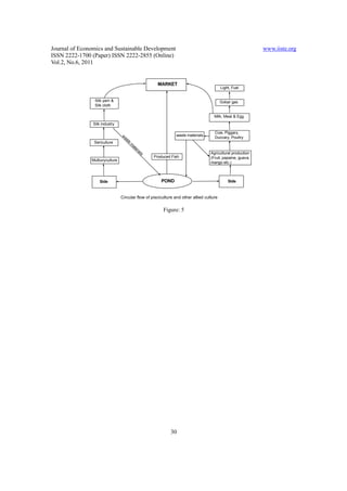
2. Sustainable development and Pisciculture

Sustainable development is a pattern of resource use that aims to meet human needs while preserving
the environment so that these needs can be met not only in the present, but also for future generations. The
term was used by the Brundtland Commission which coined what has become the most often-quoted
definition of sustainable development as development that “meets the needs of the present without
compromising the ability of future generations to meet their own needs”. It is usually noted that this
requires the reconciliation of environmental, social and economic demands - the “three pillars” of
sustainability. This view has been expressed as an illustration using three overlapping ellipses indicating
that the three pillars of sustainability are not mutually exclusive and can be mutually
reinforcing. Sustainable development ties together concern for the carrying capacity of natural systems with
the social challenges facing humanity. As early as the 1970s “sustainability” was employed to describe an
economy in equilibrium with basic ecological support systems [Wikipedia]. A primary goal of sustainable
development is to achieve a reasonable and equitable distributed level of economic well being that can be
perpetuated continually for next generation. Thus the field of sustainable development can be broken into
three constituent parts i.e. environmental, economic and social sustainability. It is proved that socio-
economic sustainability is depended on environmental sustainability because the socio- economic aspects,
like agriculture, transport, settlement, and other demographic factors are born and raised up in the
environmental system. All the environmental set up is depended on a piece of land where it exists.

Water is a renewable natural resource and is a free gift of nature. In the early days the supply
of water was plenty in relation to its demand and the price of water was very low or even zero but in course
of time the scenario has totally changed (Bairagya R. and Bairagya H. 2011). Water is a prime need for
human survival and also an essential input for the development of the nation. For sustainable development
management of water resources is very important today. Due to rapid growth of population, expansion of
industries, rapid urbanization etc. the demand of water rises many-fold which is unbearable in relation to its
resources in the earth. All the environmental set up is depended on a piece of land where it exists. So, to get
sustainable environmental management, sustainable land management is necessary. As a result the use of
water resources in the form pisciculture in a sustainable manner may gain priority.

4. Importance of the study

Social scientists have always identified the rural areas for investigation. In the case of India to a large
number of studies have been carried out in rural situations including panchayats and co-operative societies.
Though many research works have been done in the biological and marine sciences, the economic
investigations of pisciculture have not yet been done so far. In this respect the present study has a clear
economic importance for the upliftment of the rural economy at the grass root level. Thus pisciculture has a
positive effect on ecology and hence to maintain ecological balance a meaningful use of unused water
resources has an important role. Scarcity of water is a modern day tragedy human society will exist no more
16

Vol.2, No.6, 2011

due to these scarce resources. So a meaningful use of this resources in the form of pisciculture to generate
income of the rural poor gain topmost priority.

The state of West Bengal plays an important role for the implementation of the programme. Though the two
districts Burdwan and Birbhum of W.B. are primarily agricultural districts, there is huge scope for
pisciculture. A few studies have been undertaken by several experts, notably, D. Prasad (1968), R. Charan
(1981), A.V. Natarajan (1985), K. M. B. Rahim (1992,93), A Chakravorty (1996), I Guha and R. Neogy
(1996), P.K. Ghosh (1998) and others on the economic evaluation of pisciculture. Though these are useful
guides to researchers, yet there is ample scope for further works relating to pisciculture in the rural areas of
W.B. Besides, there is the necessity of developing studies concerning the impact of these programmes on
the rural economy. The present study is a modest attempt in remedying this inadequacy.

4.1 Objectives

This pilot study was conducted on the following objectives i) To generate employment in rural India. ii) To
rise in food supply and reduce mal-nutrition. iii) For proper utilisation of unused water resources. iv) To
maintain ecological balance in a sustainable manner. V) Identification of fish farmers suitable and willing
to develop fish farming in ponds.vi) Arranging training in organized manner and ensuring extension
services to fish farmers.

4.2 Methodology of the study

4.2.1 Selection of study area

The present study was confined to survey the rural areas of Burdwan and Birbhum districts of W. B. in
respect of implementation of the programme of Fish Farmers Development Agency (Mishra S. 1987). In
the selection of districts following considerations weighed most: i) Both the districts are covered with water
areas constituting half of the total inland water resources. ii) There is a heavy concentration of tanks and
ponds in both the districts. iii) Both the districts are considered as having one homogeneous agro-climatic
zone in view of the broad similarities of soils, climate and other features. Since they are also neighboring
districts a suitable comparison can easily be made. iv) In both the districts, the FFDA programmes are being
implemented in full fledged form by the Government authority. v) Data from both the districts can be
obtained because of my personal knowledge about the two districts.

4.2.2 Selection of sample

Keeping in view the time factor, limited fund and limited ability it was not possible to collect data from all
the recorded fish farmers of the two districts. At first 5 blocks from each district have been purposefully
selected. Then 10 recorded fish farmers from each block have been selected purposefully. Thus 50 fish
17

Vol.2, No.6, 2011

farmers from each district have been selected for interview. For comparative analysis of data each farmer
was taken as the unit. For this study data have been collected on different aspects of the programme such as
farmers’ income, water area, finance, total production, product price, cost of production, profit, duration of
training period etc. The data have been collected by personal interview method through a questionnaire.
Thus the collected data are entirely primary in nature.

4.2.3 Location map of the study area

The state of West Bengal lies between latitude 21038/ to 27010/ North and longitude 85038/ to 89050/ East.
The district Burdwan lies between 22056/ and 25053/ North latitude and 86048/ and 88025/ East longitude.
The district Birbhum lies between 23032/30// and 24035/00// North Latitudes and 88001/40// and 87005/25//
East Longitudes shown in figure-1.

5. Fisheries in India

Indian fisheries can broadly be divided into two categories: i) Inland fisheries & ii) Marine fisheries.
Further Inland fisheries can be classified into two types: i) Capture & ii) Culture. Capture fisheries consist
of rivers, lakes canals etc. where farmers do not cultivate fishes. Natural breeding process is the common
phenomenon there. On the other hand, culture fisheries consist of ponds, tanks, swamps, marshes etc. In
this case, farmers have to sow fish seeds, nurse it and send it to proper size before harvesting. India is the
third largest producer of fish in the world and the second in inland fish production. Indian fishing resources
comprising of 2 million sq.km.of EEZ for deep sea fishing, 7,520 km. of coast line, 29,000 km. of Rivers,
1.7 million Ha. of reservoirs, 1 million Ha. of brackish water and .8 million Ha. of ponds, lakes and tanks
for inland and marine fish production (Giriappa S. (ed) 1994) . About 14 million fishermen draw their
livelihood from fishery. During the period 1981 to 2002 the contribution of fishery to GDP has increased
from Rs.1230 crores to Rs.32060 crores. The fish production increased from 0.7 million tons in1951 to 6.8
million tons in 2006.

5.1 Fisheries in West Bengal

West Bengal has a vast water resource potentiality. By utilizing these water resources there is a huge
prospect of pisciculture (Chakraborty S. K.1991). These resources can be divided into two categories: i)
Inland water resources and ii) Marine water resources. Inland resources constitute ponds, rivers, marshy
lands, canals, reservoirs etc. Water Resources of West Bengal shown in figure-2.

It should be noted that tanks/ponds occupy the major share i.e. 46.70% of total inland water resources. But
out of 2, 76,202 Ha. area under ponds and tanks only 2, 20,000 Ha. i.e. 79.65% are presently used for
pisciculture which means 20.35% remains unused. Moreover, out of 5, 91,476.71 Ha. total inland water
resource only 2.87000 Ha. water area is brought under pisciculture i.e. 48.56% are presently used and
51.44% remains unused. These unused water resources can be brought under pisciculture through proper
utilization.
18

Vol.2, No.6, 2011

In West Bengal marine fishery has a substantial share amounting to a coast line of 158 km. inshore area up
to 10 fathoms depth is 770 sq. km. (Mamoria C.B. 1979), offshore area (10-40) fathoms depth is 1813 sq.
km. and a continental shelf up to 100 Fathom is 17,049 sq.km. Out of 19 districts of West Bengal only two
districts East- Midnapur and South 24-Parganas are coastal. West Bengal is on the top of the list in fish
production in the country. With the passage of time, more and more people are getting themselves involved
in fishery. As fish constitutes the staple food of the people efforts are being made to augment fish
production.

From the period 1986 to 2000, the total fish production increased from 424000 tons to 1045,000 tons (i.e.
2.46 times). At the same period the inland fish production increased 2.25 times and marine fish production
increased 4.50 times. In the year 1986, the share of inland and marine fisheries to total fish production were
91% and 9% respectively. But in the year 2000, the share of inland and marine fisheries to total fish
production are 83% and 17% respectively. Thus we see that during the period 1986 to 2000, the share of
inland fish to total production declined (from 91% in 1986 to 83% in 2000) and the share of marine
fisheries increased (from 9% in 1986 to 17% in 2000).

Not only in fish production but also in the demand for fish West Bengal is the highest in the country. The
domestic demand for fish in West Bengal is high because almost all the people of West Bengal are
fish-eating. But the state has a higher demand for fish than its production of fish i.e. this state has a deficit
in fish supply. To meet this gap the state West Bengal has to import fish from other states like Andhra
Pradesh, Tamil Nadu etc. At the same time various efforts have been made to augment fish production to
bridge this gap.

5.2 Fisheries in Burdwan district

The district of Burdwan is mainly an agricultural district though it is also well advanced in industrial
production. It is called the ‘granary’ of West Bengal. The district is filled with well fertile productive land.
Not only that, the district is also well endowed with a large number of water bodies in the form of rivers,
ditches, canals, marshy lands, ponds, tanks etc. The principal rivers are Ajoy, Damodar and Kunur etc.
There is a good prospect of pisciculture by utilizing these water resources. The distribution of total water
resources in Burdwan district (i.e. 66480.82 Ha.) is shown in figure-3.

Though the district has huge water resources, during the period 1982-1998 only 50% of this water area was
brought under scientific pisciculture. In the year 1999, the district’s total fish production was 55,500 metric
tons while demand in that year was 65,000 metric tons. Thus there was a deficit of 9,500 metric tons. To
meet this demand the district had to import fish from neighboring states. The district will be self-sufficient
in fish production if the unused 50% water resources are brought under pisciculture.

5.3 Fisheries in Birbhum district

19

Vol.2, No.6, 2011

The district of Birbhum is a part of Rarh area. The district is well-drained by a number of rivers and rivulets.
The principal rivers of this district are: Ajoy, Brahmani, Dwarka, Kopai, Mayurakshi etc. But most of the
rivers remain dried up during a greater part of the year. Due to this adverse natural factor pisciculture has not
made any significant progress in this district. Agriculture is the main occupation of the common people of
this district. The main water areas for pisciculture of this district are rivers, tanks, ponds, khals, Bills, baors,
reservoirs etc. The distribution of total water resources in Birbhum district (i.e. 45215.81 Ha.) is shown in
figure-4.

The figure-4 shows that this district has a large number of water resources. But during the period 1980-1999,
only 46% of this water area was brought under pisciculture through FFDA. So there is a huge prospect of
pisciculture by utilizing these unused water resources. In the year 1999 total number of fish farmers in this
district was 2, 00747 out of which 56.5% were males and 43.5% were females. The total number of fisherman
family in this district was 4,975. The average fish production of this district was 21,000 metric tons and the
annual demand was 24,000 metric tons. Thus the district had a deficit (3000 mt) in fish production. To meet
its own demand the district has also to import fish from the neighbouring states.

6. Findings

6.1 Income distribution of sample fish farmers before and after assistance from FFDA

It was observed that 26 farmers in Burdwan district & 32 farmers in Birbhum district have pisciculture as
the main occupation while others have pisciculture as a subsidiary occupation. Their basic occupations are
agriculture, business and service and have various types of incomes from those occupations. But as income
generation scheme only income from fishery was taken into account i.e. income means income earned from
selling fishes. From sample survey we have collected two sets of income data (one showing income before
and other showing income after the assistance of FFDA) for each fish farmer. Thus the amount of income
reveals the income of the fish farmer before the receipt of assistance of FFDA and the income after the
assistance of FFDA. In this regard the income comparison has done in two areas (namely within the
district, between the district and the overall change of income) and‘t’ (Gujarati D.N. 2009) test was used for
statistical analysis. Now the various types of incomes distribution of fish farmers of the two districts are
shown in terms of four tables.

From table- 1 it is clear in both the districts the average income of most of the fish farmers (i.e. 89 out of
100 fish farmers of the two districts taken together) has monthly income before assistance below Rs. 4000
i.e. they are basically come from poor family income group

i) From the field survey we get that the per capita availability of fish in Burdwan district is 24 kg. per head
per year while in Birbhum district it is 23.5 kg. per head per year. Now the world’s per capita availability of
fish is 11.5 kg. per head per year and for developed countries it is 25 kg. per head per year. But India has a
low per capita availability of 3.5 kg. per head per year only. Thus we see that the fishermen have a standard
level of per capita fish consumption. The point is very important to reduce mal-nutrition (which is a
common phenomenon for the country) by means of intensive pisciculture. But India has a poor per capita

20

Vol.2, No.6, 2011

availability of fish of only 3.5 kg per head per year. Thus we see that the per capita availability of fish for
these 100 farmers’ families of these two districts are much higher than that of India and world’s average
and even equal to the standard of the developed countries.

ii) It was found that the average monthly income of fish farmers before the assistance of FFDA in Burdwan
district was Rs. 2680 and in Birbhum district it was Rs. 2045. But after the assistance of FFDA the average
monthly incomes of the fish farmers of the two districts increased to Rs.3935 and Rs.3721 respectively.
Thus we see that the average monthly income of fish farmers of Burdwan district has increased 1.47 times
and in case of Birbhum district it has increased 1.8 times. The result indicates that the average income of
fish farmers of Burdwan district was higher than the average income of those of Birbhum district in respect
of both before and after the assistance of FFDA. However, the rate of increment was higher in Birbhum
than that of Burdwan district. Thus we can say that the incomes of the fish farmers have improved due to
pisciculture.

iii) Statistical methods were adopted is to judge whether the change of income of the sample fish farmers
before and after the assistance of FFDA was significant or not. This has been done in two areas: - a) Change
of income within the district and b) Overall change of income of the two districts.

6.2 Change of income within the district

Burdwan district- It is seen that the value of‘t’ = 3.31 is significant at .01 level, meaning thereby that the
change income of sample fish farmers of Burdwan district is significant. The gain is in favor of the
assistance of FFDA. It may be concluded from the result that there is a positive impact of assistance on fish
farming (i.e. the production of fish). It may also be concluded that production has increased significantly in
Burdwan district.

Birbhum district-The result indicates that “t” is significant at .01 level. Hence it may be said that in
Birbhum district the change of income of fish farmers is significant.

6.3 Overall change of income taking the two districts together

It is seen from the above table that the value of‘t’ is significant at .01 level which indicates that the income
of fish farmers before and after assistance differ significantly. The result reveals that the mean income after
assistance is significantly greater than that before assistance. It may be concluded from the overall results
considering both the districts that the impact of assistance on fish production is significant.

The finding of these results was that the assistance of FFDA programme has raised the fish farmer’s income
undoubtedly in both the districts. Not only that the change of income was statistically significant but also
the result revealed that there was a positive impact of FFDA assistance on fish production (i.e. fish
21

Vol.2, No.6, 2011

production has significantly increased). Moreover, it was also found that the gain of income of fish farmers
of Birbhum district was higher than that of Burdwan district. Thus we can conclude that in case of the
implementation of the programme of FFDA the district Burdwan has more successful achievements than
the district of Birbhum.

7 Suggestions

7.1 General suggestions

i) In pisciculture, fishermen are not only directly employed in fishing but also some other alternative
occupations like net making, marketing of fish seed and fishery product , transport, boat making etc. many
rural people earn income. Since fish is a perishable commodity proper marketing channels should be
established. Hence to reduce pressure from agriculture pisciculture may be alternative occupations for
generating income and employment for a large number of poor people. ii) In Burdwan district there are
some open caste pits (OCP) in Ranigang coal belt and in Birbhum district also such pits are available at
Khoirasole block, calamines at Md.Bazar block. Fish production may increase by utilizing these water
resources for pisciculture purposes.iii) The urban waste (i.e. garbage) may be recycled as fish feed (to those
ponds and water areas lying near the towns) to raise fish production and to prevent the environmental
pollution in those areas. v) To make financial support for the poor fishermen Bank should grant loan on a
long-term basis and at a low rate of interest in proper amount and in proper time.vi) the selection of actual
beneficiary is very much essential and it should be made on the basis of need and neutrally not in politically.
vii) Since fish is a perishable commodity storage facilities should be provided such that the fishermen are
not forced to sell their product at a lower price. Prices of organic manures and fish seeds should be kept as
low as possible or the Government should give more subsidies in the case of chemical fertilizers so that the
poor fish farmers can buy them. viii) For welfare measures of the rural poor fishermen some Group and
Personal Insurance Schemes, Old- Age Pension Schemes should be taken and the Fishery Dept. should
issue “Identity Card” to each fisherman. ix) Since both the districts are agricultural based we should
interlink agriculture with pisciculture shown in figure-5. Along with pisciculture in ponds other allied
culture can be inter-linked in composite farming. The concept of composite farming e.g. in the pond- there
are pisciculture and on one side of the pond mulberry trees can be cultivated for the development of
sericulture industry-from there silk industry can be grown. Thus the final products (i.e. silk yarn and silk
cloth) come to the market and their waste materials are drained off to the pond and used as fish feed. In the
same pattern on another side of the pond animal husbandry can be practiced (e.g. poultry, duccary and
piggery). Their waste can be used as a valuable manure for fish feed and the residual can be utilized for
agricultural production. The excreta of the animal husbandry can also be used in the bio-gas plant for fuel
and light. The products of animal husbandry e.g. milk, meat and egg come to the market directly. On
another side of the pond some fruit plants such as papine, guava, mango etc. can be cultivated by using the
excess manure of animal husbandry and the products can be sold in the market.

x) Composite fish culture: Stocking of various species should be in a certain proportion such that various
types of fishes live in various layers and eat the entire food organism (so called Polyculture or Composite
Fish Culture). Stocking is an important factor to raise fish production. On an average the survibility of
stocking is 80% (Jhingran V.G. 1991). This means that 20% of stocking is lost for various reasons such as
improper handling, netting and also eaten by preratory animals like snakes, frogs etc. The main species
cultured in India are Rahu, Catla, Mrigel, Silver Carp (S.C.), Grass Carp (G.C.), Cyprinus Carpio (Cy, Ca.)

22

Vol.2, No.6, 2011

and Bata etc. In polyculture (where various fishes are cultured simultaneously) (Agarwal S.C. 1990) system
all these species are cultured in certain ratios. It is found that all of these species do not generally live in the
same layer. In mixed (or polyculture or composite culture) culture all these fishes are cultured in such a way
that all layer’s feed are used. If we divide the whole layer into 3 parts i.e. upper, middle and lower layers,
then Cattla and S.C live in the upper layer, Rahu and G.C. live in the middle layer and Mrigel and Cy. Ca.
live in the lower layer. It is also to be noted that these two species in the same layer are not competitors of
each other. In their feed habit one eats waste weeds and the other eats green weeds. Hence in polyculture all
the pond’s feed are used scientifically and economically. The production of Big head and Big head African
giant hybrid magur are totally banned because their food habits are too much and hamper the foods of other
common species. Suppose 1000 fish seed is cultivated in the pond. Then the stocking ratios for various
fishes are Rahu: Catla: Mrigel: S.C.: G.C.: Cy.Car = 3 : 1 : 1.5 : 1.5 : 1 : 2 Thus the number of seeds are,
Rahu = 300, Catla = 100, Mrigel = 150, S.C = 150, G.C. = 100, Cy. Ca. = 200. Now the survibility rate is
80%.Thus the number of produced matured fishes are Rahu = 240, Catla = 80, Mrigel = 120, S.C. = 120,
G.C. = 80, Cy.Car. = 160. Fishes are cultivated for 9-12 months. The culture period may extend up to 18
months with partial harvesting between. Moreover, the general annual growth of these fishes are, Rahu =
1kg, Catla 1.5 kg. Mrigel 0.75kg, SC. = 0.8 kg, G.C. = 1.5 kg, Cy. Car. = 0.8 kg. The fish farmers collect
fish seeds from private traders or from Government fish farm.

xi) Since training is a necessary ingredient to raise fish production the Government has initiated some
special training programmes for fish farmers. Moreover to motivate the poor fish farmers some amount of
remuneration or stipend is paid to the participant during training. The amount of remuneration depends
upon the kind of training, place of training organization and duration of the training programmes conducted
by the FFDA. To attend the district level training programmes for the farmers of distant villages, traveling
allowances are also paid.

xii) It is very essential to use mahua cake because it has dual roles in pisciculture. It firstly acts as a
pesticide but later it acts as organic manure and produces a desired quantity of fish food organism for the
baby fishes. The presence of ‘Saponin’ in mahua cake kills the pre-ratory animals / fishes of the pond. This
poisonous effect continues about 10-15 days and after that it acts as manure. On the other hand, the use of
pesticides has a negative long-term effect to ecological balance. So the pesticides are not generally used
though they are cheaper. The mahua cake should be applied at the rate of 333.33kg/ Yr. / bigha.

7.2 Limitations of the study

The following are the limitations of the study: i) Regarding the change in the level of income before and
after the assistance of FFDA, the statements of the fish farmers have been taken into consideration on good
faith. ii) Due to limited time, ability and resource constraints, data have been collected from a small number
of fish farmers of the two districts and results are assumed to be the representative for the district as a
whole. Iii) Due to difficulties in getting responses from the sample fish farmers sometimes we had to rely
on the different FEOs’ opinions and also on different official records on good faith. iv) The observations
made on the basis of collected data are obviously particularistic in nature in so far as these data relate to
micro-study like the present one (i.e. only 100 fish farmers from the two districts were taken into
consideration). Micro-studies do not attempt to build general theories but the utility of this type of study is
that large number micro-studies may, in course of time, be helpful in constructing meaningful
generalizations. Moreover, it is an explorative study which seeks to explore the conditions of fish farmers

23

Vol.2, No.6, 2011

before and after the assistance of FFDA programme. A much larger study may be undertaken to vindicate
the results obtained from this explorative study.

8. Conclusion

The study indicates that the introduction of the programme of FFDA had a clear positive impact on the rural
economy through employment and income generation and also raising the standard of living and
socio-economic performances of the rural community of the two districts. It is environmentally viable,
sustainable and eco-friendly in nature. So for sustainable use of the scarce water resources it is very
essential in the present context. Unemployment is a curse for the society today and pressure of population
on agricultural sector is rising day by day. Thus fish farming may be an alternative occupation for those
unemployed people and undoubtedly generate income in a viable method. Therefore it is recommended that
the present programme should be further spread in the rural areas by means of proper planning, adequate
supervision, effective implementation and better monitoring in a sustainable manner.

References:

Agarwal S.C. (1990), Fishery Management, Ashis Publishing House, New-Delhi.

Bairagya R. and Bairagya H. (2011), “Water Scarcity a Global Problem- An Economic Analysis”,
Indian Journal of Landscape Systems and Ecological Studies, Vol.-34, Institute of Landscape, Ecology &
Ekistics, Kolkata, 127-132

Bairagya R. (2004), “A Comparative Study of the Functioning of Fish Farmers Development
Agency (FFDA) in the Districts of Burdwan and Birbhum (1985-1995)”, PhD Thesis, Department of
Commerce, the University of Burdwan.

Bureau of Applied Economics, Burdwan (1998), Key Statistics of Burdwan, Govt. of W.B.

Bureau of Applied Economics, Birbhum (1998), Key Statistics of Birbhum, Govt. of W.B

Chakraborty S. K. (1991), A Study in Bhery Fisheries, Agro-Economic Reaserch Centre, Visva- Bharati.

Dutt R. and Sundharam K.P.M. (2009), Indian Economy, S. Chand and Co. New-Delhi, 101-103

Jhingran V.G. (1991), Fish and Fisheries in India, Hindustan Publishing Cor.-Delhi.

Giriappa S. (ed) (1994), Role of Fisheries in Rural Development, Daya Publishing House, Delhi.

Gujarati D.N. (2009), Basic Econometrics, McGraw-Hill., 98-133

Mamoria C.B. (1979), Economic & Commercial Geography of India, Shiblal Agarwala Company, Agra-3

Mishra S. (1987), Fisheries in India, Ashis Publishing House, New-Delhi

Acknowledgement: In preparation of this paper I deeply acknowledge my respected sir Prof. Jaydeb
Sarkhel, Department of Commerce, Burdwan University, West Bengal, India, e-mail:

24

Vol.2, No.6, 2011

jaydebsarkhel@gmail.com

Tables and Figures:

Figure-1

25

Vol.2, No.6, 2011

26

Vol.2, No.6, 2011

Figure-2

Figure-3 Figure-4

Table -1 Change of income distribution of Burdwan.

27

Vol.2, No.6, 2011

Table -2 Change of income distribution of Birbhum district

Table--3 Classification of sample fish farmers according to their monthly incomes after the assistance

28

Vol.2, No.6, 2011

Table- 4 Classification of sample fish farmers according to their monthly incomes after the assistance

Source: All tables data sources are computed from field survey.

29

Vol.2, No.6, 2011

MARKET
Light, Fuel

Silk yarn & Gobar gas
Silk cloth

Milk, Meat & Egg
Silk industry

Cow, Piggary,
waste materials
Duccary, Poultry
w
as

Sericulture
te
m
at
er
ia

Agricultural production
ls

Produced Fish (Fruit, papaine, guava,
Mulburyculture
mango etc.)

Side POND Side

Circular flow of pisciculture and other allied culture

Figure: 5

30

Vol.2, No.6, 2011

The Nexus of Private Savings and Economic Growth in
Emerging Economy: A Case of Nigeria
Adelakun, Ojo Johnson
Department of Economics, Joseph Ayo Babalola University
P.M.B. 5006, Ilesa, Osun State, Nigeria, email joadelakun@yahoo.co.uk


Abstract
This study discusses the trend in Nigerian saving behaviour and reviews policy options to increase
domestic saving. It also examines the determinants of private saving in Nigeria during the period covering
1970 – 2007. It makes an important contribution to the literature by evaluating the magnitude and direction
of the effects of the following key policy and non-policy variables on private saving: Income growth,
interest rate, fiscal policy, and financial development. The framework for analysis involves the estimation
of a saving rate function derived from the Life Cycle Hypothesis while taking into cognizance the structural
characteristics of a developing economy. The study employs the Error-Correction modelling procedure
which minimizes the possibility of estimating spurious relations, while at the same time retaining long-run
information. The results of the analysis show that the saving rate rises with both the growth rate of
disposable income and the real interest rate on bank deposits. Public saving seems not to crowd out private
saving; suggesting that government policies aimed at improving the fiscal balance has the potential of
bringing about a substantial increase in the national saving rate. Finally, the degree of financial depth has a
negative but insignificant impact on saving behaviour in Nigeria.
Keywords: Private Saving, Saving Rate, Macroeconomic Policy, Interest Rate, Economic Growth.

Introduction
Researchers and policy makers are known to be having growing concern among researchers and policy
makers over the declining trend in saving rates and its substantial divergence among countries. This is due
to the critical importance of saving for the maintenance of strong and sustainable growth in the world
economy. Over the past three decades, saving rates have doubled in East Asia and stagnated in Sub-Saharan
Africa, Latin America and the Caribbean (Loayza, Schmidt-Hebbel and Serven, 2000). The personal saving
rate has been drifting downward for the last two decades. According to the latest statistics, personal saving
declined from about 10% of disposable income in the early 1980s to 1.8% in 2004. The decline has
received particular attention recently because saving was negative in 2005 for the first time since the Great
Depression. Although saving declined in other developed countries during this period, the U.S decline was
more pronounced than in most of the three countries.
Development economists have been concerned for decades about the crucial role of domestic
saving mobilization in the sustenance and reinforcement of the saving-investment-growth chain in
developing economies. For instance, Aghevli et al (1990) found that the saving rate and investment in
human capital are indeed closely linked to economic growth. The relationship among saving, investment
and growth has historically been very close; hence, the unsatisfactory growth performance of several

31

Vol.2, No.6, 2011

developing countries has been attributed to poor saving and investment.
This poor growth performance has generally led to a dramatic decline in investment. Domestic
saving rates have not fared better, thus worsening the already precarious balance of payments position
(Chete, 1999). In the same vein, attempts to correct external imbalances by reducing aggregate demand
have led to a further decline in investment expenditure, thus aggravating the problem of sluggish growth
and declining saving and investment rates (Khan and Villanueva, 1991). In addition, low personal saving
has created short-run concerns that a sudden increase in the saving rate could reduce growth of consumer
spending, and output and employment.

Statement of the Problem
The strong positive correlation which exists between saving, investment and growth is well
established in the literature. The dismal growth record in most African countries, relative to other regions of
the world has been of concern to economists. This is because the growth rate registered in most African
countries is often not commensurate with the level of investment. In Nigeria for instance, the economy
witnessed tremendous growth in the 1970s and early 1980s as a result of the oil boom and this led to the
investment boom especially in the public sector. However, with the collapse of the oil market in the 1980s,
investment fell, thereby resulting in a fall in economic growth. For instance, during the investment boom,
gross investment as a percentage of Gross Domestic Product (GDP) was 16.8 and 31.4 percent in 1974 and
1976 respectively, whereas it declined to 9.5 and 8.9 percent, respectively in 1984 and 1985(CBN 2008).
One question begging for an answer is: What is the impact of saving and investment on growth? It
has been argued that saving affects investment, which in turn influences growth in output. The transformation
of initial growth into sustained output expansion requires the accumulation of capital and its corresponding
financing. An output expansion in turn sets in motion a self reinforcing process by which the anticipated
growth encourages investment, which supports growth, as well as financial development. It is certain that
without a significant increase in the level of investment (public and private), no meaningful growth in output
would be achieved. Indeed if private investment remains at the current low level, it will slow down potential
growth and reduce long run level of per capita consumption and income, thereby leading to low savings and
investment.

Objective of the Study
• This study has the following objectives:
• To know the impact of private saving in economic growth in Nigeria.
• To also carry out an analysis of the sources and trend of saving in Nigeria.
• To also know the motivations of saving and how savings are measured.
• To also know how saving affects the economic performance in the country.
• To also evaluate the impact of the main determinants of saving identified in the literature on private
saving in Nigeria.
Method of the Study (Methodology)
The framework for this analysis is derived from the life-cycle model which has withstood the test of
time in explaining the changes in private saving over time. It is appropriately modified to accommodate the
peculiarities of a developing country and builds on the existing cross-country literature on saving which
quantifies the effects of a variety of policy and non-policy variables on private saving. Its attractiveness lies
in its elegant formulation of the effects of interest rate and growth on saving. In addition, its flexibility makes
it possible for other relevant theoretical considerations to be incorporated, thus forming an integrated
analytical framework, without altering its fundamental structure. This framework makes a new contribution
to the literature by employing time series data in evaluating the determinants of private saving in Nigeria

32

Vol.2, No.6, 2011

between 1970 and 2009. It does this while explicitly addressing some of the econometric problems arising
from the use of time-series data.

Literature Review, Theoretical Framework and Empirical Evidence
Introduction
Keynes (1936) defined savings as the excess of income over expenditure on consumption.
Meaning that savings is that part of the disposable income of the period which has not passed into
consumption (Umoh, 2003 and Uremadu, 2005). Given that income is equal to the value of current output;
and that current investment (i.e. Gross capital formation) is equal to the value of that part of current output,
which is not consumed; savings is equal to the excess of income over consumption. Hence, the equality of
savings and investment necessarily follow thus:
Income = Value of output = Consumption + Investment
Savings = Income – Consumption
Savings = Investment ex-post.
There abound numerous theoretical evidences concerning the functional relationships between
savings and a wide range of causal variables. For instance, Juster and Taylor (1975) report that savings is an
increasing function of income. Moreover, Modigliani (1970), Madison (1992), Bosworth (1993), Caroll and
Weil (1993), Schmidt-Hebbel, Sarven and Solimano (1994), Modigliani (1992), Jappeli and Pugano (1994),
Edwards (1995), Collins (1991) and Uremadu (2000) maintain that there exists a positive relationship
between savings and income growth rates. Aghevli (1990) in Ozigbo (1999) reported that there is consensus
that the level of savings is largely determined by the level of income.
In Nigeria and other developing economies, there are other evidences that interest rate has significant
effect on financial savings especially time and savings deposits while the structure of deposits was
determined by differentials in deposit rates as has been demonstrated in Ndekwu, (1991). He also showed
using monthly data that interest rates deregulation in Nigeria have a positive impact on financial savings
during the period, 1984-1988.
Literature Survey
Franco Modigliani in his Life Cycle model determined that over the typical individual’s lifetime
his level of income will fluctuate from low levels in his younger years, to high levels in his middle-aged
working years, back to low levels in his retirement years. However, this individual prefers to maintain a
relatively stable level of consumption. In order to maintain this steady consumption, the individual will be
forced to borrow during his younger years, save during his middle-aged years and then spend down his
savings in his retirement years. From estimating his model, Modigliani concludes that individuals have a
marginal propensity to consume (MPC) out of income of approximately 0.70 and an MPC out of net worth
if approximately 0.07 to 0.08. (Ando and Modigliani, 1962)
Many researchers have studied the possible determinants of private savings behavior. In
Amaoteng’s survey article, he shows that saving has been found to be positively correlated with income,
wealth, education, age, a high level of risk tolerance, and a favorable perception of one’s own financial
status; and negatively correlated with a larger family size. (Amaoteng 2002) Modigliani’s life cycle model
illustrates that age structure can have a strong impact on the level of savings in an economy. Since
individuals in the middle-aged working years (which we will define as ages 25-55) tend to save more than
individuals in the younger (ages 0-24) or retirement years (ages 56+), a population with a higher
concentration of individuals in the middle-aged range will have higher savings rates. (Amaoteng 2002)
Trend of Saving in Nigeria
In mobilizing funds from the surplus units of the economy, banks incur some costs mainly in interest
payments on deposit accounts. In order to recover the cost of deposit mobilization and other operating
overheads, banks lend at higher interest rates. The difference between the two types of rates is referred to as
33

Vol.2, No.6, 2011

the interest rate spread or the intermediation spread. The spread measures the efficiency of the intermediation
process in the market, such that, a high intermediation spread implies that there is inefficiency in the market,
especially as it discourages potential savers and borrowers, thus, hampering investment and growth.
Prior to the deregulation of the banking sector, interest rates were administratively determined by
the Central Bank. Both the deposit and lending rates were fixed by the CBN on the basis of policy decisions.
At that time, the major goals were socially optimum resource allocation, promotion of orderly growth of the
financial market, as well as reduction of both inflation and the internal debt service burden on the
government. During the period 1970 to 1985, the rates were unable to keep pace with prevailing inflation
rate, resulting in negative real interest rates. Moreover, the performance of the preferred sectors of the
economy was below expectation, thus, leading to the deregulation of the interest rate in August 1987 to a
market-based system. This enabled banks to determine their deposit and lending rates according to the market
conditions through negotiations with their customers.
However, the minimum rediscount rate (MRR) which is the central bank’s nominal anchor
continued to be determined by the CBN. The lack of responsiveness of the structure of deposit and lending
rates to market fundamentals makes the interest rate inefficient. The wide divergence between the deposit and
lending rates (interest rate spread) is inimical to economic growth and development of the Nigerian economy.
Between 1980 and 1984, interest rate differentials averaged 3.9 per cent. Even though this was reasonable
within the accepted limit, the spread widened between 1985 and 1989, averaging 4.3 per cent per annum. This
impacted negatively on the amount of loanable funds available to the private sector for investment.
The interest differential further widened to an average of 7.9 per cent between 1990 and 1994.
Thereafter, the yearly interest rate spread maintained an upward trend, rising from 8.2 per cent in 1995 to 24.6
per cent in 2002, before declining to 15.7 per cent in 2005 (see Figure 1). The widening gap between the
deposit and lending rates reflects the prevailing inefficiencies in the Nigerian banking sector and has deterred
potential investors from borrowing, and thus lowered the level of investment in the economy.

Interest Rate Spread (in Percentage)
Source: Central Bank of Nigeria i) Statistical Bulletin, 2006 and
ii) Annual Report and Statement of Accounts, various years.
The use of interest rate spread has however been criticized given that higher levels of interest rates
are usually associated with higher inflation rates, and therefore a higher cost of holding money. In addition,
higher inflation rates tend to be associated with higher country premia. As a result of these disadvantages of
interest rate spread as an indicator of efficiency, net interest margin has been proposed as a better alternative.
Net interest margin is equal to total interest revenues minus total interest expenditure divided by the value of
assets. Higher values of net interest margin indicate a higher spread on deposit and lending rates and therefore
lower efficiency.

Figure 2 shows the interest rate figures in Nigeria between 1970 and 2009. A cursory look reveals
that the nominal interest rate was institutionally determined by the monetary authorities throughout the 1970s
and the first half of the 1980s. However, with the advent of the structural adjustment programme in the mid
1980s which brought with it a rash of financial sector reforms, Nigeria abandoned its fixed interest rate
regime that saw nominal interest rates rising from 9.3 percent in 1985 to 26.8 percent in 1989, and reaching a
peak of 29.8 percent in 1992. The figure has since hovered between 13.5 percent and 24.4 percent. It stood at
16.5 percent in 2009.

Real Interest Rate (in Percentage)
Source: Central Bank of Nigeria i) Statistical Bulletin, 2006 and
34

Vol.2, No.6, 2011

The real interest rate figures present an interesting picture. Between 1970 and 2009, the figure was
negative 20 times, attaining positive figures on 18 occasions. The fixed interest rate regime of the 1970s and
early 1980s no doubt contributed to this negative trend by fixing the interest rate at artificially low levels. For
instance, in the first two decades (1970 to 1989) when the fixed regime dominated, real interest rate was
negative 14 times and positive only 6 times. However, in the last two decades (1990 to 2009), when market
forces took over, the real interest rate was negative on only 6 occasions. The inflation rate also played a very
important role in making the real interest rate negative for most of the period. A cursory glance at figure 2
shows that the years when the real
interest rate was negative usually
coincided with those of double-digit
inflation rates.
Table 1 shows the components
of saving in Nigeria including savings
and time deposits with deposit money
banks, the national provident fund,
federal savings bank, federal mortgage
bank, life insurance funds and other
deposit institutions. Saving and time
deposits in banks is by far the single most
important component of saving in

Nigeria and has witnessed a continuous
growth over the years. Beginning with a
sum of N337 million in 1970, it rose to
N5.2 billion in 1980. By 1990, the figure
had climbed to N23.1 billion, rising
further by 2000 to N343.2 billion. As at
2005, the figure stood at N1.3 trillion.
Its contribution to total saving
has however been mixed. In 1970,
savings in banks consisted of 98.8 percent
of total saving, with this figure reducing
gradually to 89.5 percent in 1980, and
further declining to 78 percent in 1990.
From then the percentage of savings in
banks in total saving has witnessed an
upward trend, rising to 89.1 percent in
2000. Since 2003, this percentage has
been 100 percent showing that it has
become the only component of saving.
The National Provident Fund
and the Federal Mortgage bank were both
established in 1974. Beginning with
N130 million, the National Provident
Fund rose to N724 million in 1990,
reaching a peak of N1.37 billion in 1998.
The fund maintained this figure till 2002
when it was scrapped by the government.
The Federal Mortgage Bank on the other
hand experienced a more rapid growth,
rising from a paltry N7.3 million at its inception in 1974 to N305 million in 1990. By 2002 when it ceased to
35

Vol.2, No.6, 2011

exist, it had mobilized N22.3 billion. The figures for the Federal Savings Bank have been mixed. It stood at
N4.9 million in 1970, increasing to N8.1 million in 1978. It thereafter declined to N4.0 billion in 1982, after
which the figure climbed steadily till it reached N37.5 billion in 1989 when it was discontinued. Life
insurance funds were established in the same year 1989 with the sum of N1.1 billion. The figure rose sharply
to N19.4 billion in 1994 thereafter witnessing a rapid decline. The amount mobilized stood at N8.5 billion in
2002 when the federal government scrapped it.

Savings, Growth and Fiscal Deficit (in percent)
Notes:
i) Savings is the ratio of private saving to Gross National Disposable Income (GDNI);
ii) Growth is the growth rate of real per capita GNDI;
iii) Fiscal Balance is the surplus or deficit of the entire federation as a percentage of GDP.
Source: Central Bank of Nigeria
i) Statistical Bulletin, 2006 and
Figure 3 shows the other macroeconomic variables of interest, including private saving rate, growth
and fiscal balance. The Nigerian economy has witnessed several fluctuations in its chequered history, with
economic growth fluctuating between 45 percent and -31 percent in the period between 1970 and 2009. In the
27 year period between 1974 and 2001, the economy experienced negative growth 14 times, while making a
positive showing only 13 times. However, growth has been positive since 2002. Fiscal balance was even
more troubling given that Nigeria experienced a budget surplus only six times out of the 38 year period
between 1970 and 2009. The State governments have been as culpable as the government at the centre, with
each level seemingly competing to outspend the other.
Private saving witnessed much less volatility, with the variable recording a negative value only once
in the 38 year period. The saving rate fluctuated between 20 percent and 41 percent between 1970 and 1979.
This figures changed to 14 percent and 36 percent in the next decade. Between 1990 and 1999, the saving rate
hovered between -0.6 percent and 39 percent, reaching an impressive range of between 20 percent and 65
percent in the period 2000 to 2009. The private saving rate stood at 58 percent in 2009.
Theoretical Framework
The life-cycle hypothesis was formulated by Modigliani (1970) and is the principal theoretical
underpinning that has guided the study of savings behaviour over the years. A critical analysis of this theory
however shows that it seems to mirror what happens in developed economies with little or no regard to the
peculiarities of developing countries like Nigeria. There are a number of reasons that make it imperative for
saving behaviour in developing countries to be modelled separately from that in developed economies. First,
at the microeconomic level, developing-country households tend to be large and poor. They have a different
demographic structure, more of them are likely to be engaged in agriculture, and their income prospects are
much more uncertain. The problem of allocating income over time thus looks rather different in the two
contexts, and the same basic models have different implications for behaviour and policy.
Second, at the macroeconomic level, both developing and developed countries are concerned with
saving and growth, with the possible distortion of aggregate saving, and with saving as a measure of
economic performance. However, few developing countries possess the sort of fiscal system that permits
deliberate manipulation of personal disposable income to help stabilize output and employment. Third, much
of the literature in the last five decades expresses the belief that saving is too low, and that development and
growth are impeded by the shortfall. Sometimes the problem is blamed on the lack of government policy,
other times on misguided policy. Lastly, saving is even more difficult to measure in developing than in
advanced economies, whether at the household level or as a macroeconomic aggregate. The resulting data
inadequacies are pervasive and have seriously hampered progress in answering basic questions.
36

Vol.2, No.6, 2011

Given the above, and following Deaton (1989), this paper appropriately modifies the life-cycle
theory by developing a model of households which cannot borrow but which accumulate assets as a buffer
stock to protect consumption when incomes are low. Such households dissave as often as they save, do not
accumulate assets over the long term, and have on average very small asset holdings. However, their
consumption is markedly smoother than their income.
Following McKinnon (1973) and Shaw (1973), we argue that for the typical developing country, the
net impact of a change in real interest rate on saving is likely to be positive. This is because, in the typical
developing economy where there is no robust market for stocks and bonds, cash balances and quasi-monetary
assets usually account for a greater proportion of household saving compared to that in developed countries.
In addition, in an environment where self-financing and bank loans constitute the major source of investment
funds, accumulation of financial saving is driven mainly by the decision to invest and not by the desire to live
on interest income. Given the peculiarities of saving behaviour, in addition to the fact that the bulk of saving
comes from small savers, the substitution effect is usually larger than the income effect of an interest rate
change.
Empirical Evidence
There is an abundance of empirical studies that deal with the impact of the different variables of
interest on savings mobilization. Some authors have found a strong positive relationship between real per
capita growth and saving rates (see for example, Modigliani, 1970; Bosworth, 1993; and Carrol and Weil,
1994). However, its structural interpretation is controversial, since it is viewed both as evidence that growth
drives saving (Modigliani, 1970; and Carrol and Weil, 1994) and that saving drives growth through the
saving-investment link (Levine and Renelt, 1992; and Mankiw, Romer and Weil, 1992).
Given the importance of controlling for the joint endogeneity of saving and income growth, a panel
instrumental-variable approach to estimate the effect of income growth on saving was carried out by Loayza,
Schmidt-Hebbel, and Serven (2000). They found that a one percentage point rise in growth rate increases the
private saving rate by a similar amount, although this effect may be partly transitory. In their study, they
utilized the world saving database, whose broad coverage makes it the largest and most systematic collection
of annual time series on country saving rates and saving-related variables, spanning 35 years (1960 – 1994)
and 134 countries (112 developing and 12 industrial). Obadan and Odusola (2001) employed both graphical
analysis as well as Granger Causality tests to determine the impact of growth on saving. Their results
revealed that growth of income does not Granger-cause saving, suggesting that saving is not income-induced
in Nigeria. Evidence on the reverse causation argument also shows that saving does not Granger-cause
growth. The findings therefore do not show any direct relationship between saving and income growth.
Analytically, the effect of financial liberalization on private saving rates works through the
expansion of the supply of credit to previously credit-constrained private agents. This allows households and
small firms to use collateral more widely, and reduces down payments on loans for consumer durables and
housing. Quantitative evidence strongly supports the theoretical prediction that the expansion of credit should
reduce private saving as individuals are able to finance higher consumption at their current income level.
Loayza, Schmidt-Hebbel, and Serven (2000), find that a 1 percentage point increase in the ratio of private
credit flows to income reduces the long-term private saving rate by 0.75 percentage point. Bandiera and
others (2000), on carrying out a deeper analysis of eight episodes of financial liberalization, failed to find a
systematic direct effect on saving rate: it was positive in some cases (Ghana and Turkey), clearly negative in
others (Mexico and Korea), and negligible in the rest.
These studies however, have a number of shortcomings. To begin with, each of them focuses on
only one of the determinants of saving. They therefore do not identify the determinants of saving and analyze
their impact on the saving rate. In addition, the conclusion of Essien and Onwioduokit (1998) should be taken
with a measure of caution. This is because the time span of their study is relatively short (1987-1993). It is
therefore difficult to separate the effect of financial development from the effect of recovery and increased
capital inflow to the economy, all of which were taking place concurrently. Our study will try to overcome
this problem of simultaneity by using a longer time frame dating from 1970-2009.

37

Vol.2, No.6, 2011

Research Methodology
The methodology used in this study is the Cointegration and Error-Correction Methodology (ECM).
The ECM is made up of models in both levels and differences of variables and is compatible with long-run
equilibrium behaviour.
Model Specification
Drawing from the analysis above on the life cycle framework, the following model was specified:
PSR= β0 + β1GRCY +β2RIR + β3FB + β4DFD + ε
Where: β1 β2 and β4 ˃0, while β3 ˂ 0 and
PSR = private saving rate
GRCY = growth rate of real per capita GNDI
RIR = real interest rate
FB = fiscal balance
DFD = degree of financial depth
The saving equation was estimated using annual data for the period 1970-2009. The estimation
period was determined largely by the availability of adequate data on all variables.
Descriptive Statistics.
The characteristics of the distribution of the variables are presented in Table 1 below. Jarque-Bera is a
test statistic for testing whether the series is normally distributed. The test statistic measures the difference of
the skewness and the kurtosis of the series with those from the normal distribution. Evidently, the
Jarque-Bera statistic rejects the null hypothesis of normal distribution for the real interest rate. On the
contrary, the null hypothesis of normal distribution is accepted for degree of financial depth, fiscal balance,
income growth and private saving.
In Nigeria, as in most developing countries, due to the absence of detailed statistical coverage of
sectoral financial activity, most of the data on saving are obtained from the national accounts statistics as
the difference between measurable aggregates. This residual or indirect approach to the calculation of
saving has some drawbacks. First, the saving of one group of economic units used by another for
consumption is not captured. Second, capital gains and losses induced by price changes are not treated
adequately. Third, consumer durables and certain elements of government expenditure are also not
adequately treated (see Shafer, Elmeskov, and Tease, 1992). For these reasons, the results obtained should
be interpreted with caution.
Table 2. Summary of the Descriptive Statistics of the Variables
DFD FB GRCY PSR RIR
Mean 24.24 -3.46 2.02 28.69 -5.31
Median 24.00 -3.50 3.00 26.00 -0.60
Maximum 35.00 9.80 45.00 65.00 18.00
Minimum 12.00 -11.10 -31.00 -0.60 -52.60
Std. Dev. 6.39 4.29 17.84 12.79 16.01
Skewness -0.07 0.52 0.48 0.56 -1.05
Kurtosis 2.009 4.01 3.33 4.05 3.74
Jarque-Bera 1.54 3.24 1.61 3.65 7.61
Probability 0.46 0.20 0.45 0.16 0.02

38

Vol.2, No.6, 2011

Sum 897.00 -127.99 74.70 1061.40 -196.40
Sum Sq. Dev. 1472.81 661.12 11459.88 5886.52 9229.21
Observations 37 37 37 37 37

Source: National accounts statistics
Results of Stationarity Tests
Testing for the existence of unit roots is a principal concern in the study of time series models and
cointegration. The presence of a unit root implies that the time series under investigation is non-stationary;
while the absence of a unit roots shows that the stochastic process is stationary (see Iyoha and Ekanem,
2002). The time series behaviour of each of the series using the Augmented Dickey-Fuller and
Phillips-Perron tests are presented in Tables 3 and 4, respectively. The results show that while the private
saving rate (PSR), growth rate of real per capita GNDI (GRCY) and fiscal balance (FB) are I(0) variables
(stationary before differencing), real interest rate (RIR) and the degree of financial depth (DFD) are I(1)
variables (stationary after first differencing). This is deduced from the fact that the absolute values of both the
ADF and PP test statistics of RIR, GRCY and FB before differencing are greater than the absolute value of
the critical values at the 1 percent significance level. For the other variables, this is the case only after
differencing once.
Table 3. Results of Augmented Dickey Fuller (ADF) Unit Root Test
Variable ADF Value ADF Value Critical Value Level of
before After Integration
Differencing Differencing
PSR -3.657* n.a 3.621 I(0)
GRCY -5.068* n.a 3.627 I(0)
RIR -3.204 -6.275* 3.621 I(1)
FB -4.450* n.a 3.621 I(0)
DFD -1.979 -5.784* 3.621 I(1)

Notes: * denotes significant at 1 percent; the null hypothesis is that there is a unit root. n.a = not applicable

Table 4. Results of Phillips-Perron (PP) Unit Root Test
Variable PP Value PP Value After Critical Value Level of
Before Differencing Integration
Differencing
PSR -3.683* n.a 3.621 I(0)
GRCY -5.019* n.a 3.627 I(0)
RIR -3.045 -13.017* 3.621 I(1)
FB -4.405* n.a 3.621 I(0)
DFD -2.047 -5.784* 3.621 I(1)

Notes: * denotes significant at 1 percent; the null hypothesis is that there is a unit root. n.a = not applicable
Cointegrated Models

39

Vol.2, No.6, 2011

In this study, the method established by Johansen (see Johansen, 1991) was employed in carrying
out the cointegration test. This is a powerful cointegration test, particularly when a multivariate model is
used. Moreover, it is robust to various departures from normality in that it allows any of the five variables in
the model to be used as the dependent variable while maintaining the same cointegration results.
Accordingly, Johansen’s test was carried out to check if the saving equation is cointegrated. Table 5
shows that both the Trace and Maximum Eigen statistics rejected the null of no cointegration at the 5 percent
level; while Trace test indicated that there are two cointegrating equations at the 5 percent level; Maximum
Eigen test indicated only one cointegrating equation at the 5 percent level. The implication is that a linear
combination of all the five series was found to be stationary and thus, are said to be cointegrated. In other
words, there is a stable long-run relationship between them and so we can avoid both the spurious and
inconsistent regression problems which otherwise would occur with regression of non-stationary data series.
Table 5 Johansen’s Cointegration Test Results
Maximum Eigenvalue Test Trace Test
Null Alternative Eigen-value Critical Alternative LR Ratio Critical
Hypothesis Hypothesis Value Hypothesis Value
95% 99% 95% 99%
r=0 r=1 39.79* 37.52 r≥1 108.69** 87.31 96.58
42.36
r≤1 r=2 31.30 31.46 36.65 r≥2 68.90* 62.99 70.05
r≤2 r=3 18.02 25.54 30.34 r≥3 37.60 42.44 48.45
r≤3 r=4 16.09 18.96 23.65 r≥4 19.58 19.58 30.45
r≤4 r=5 3.49 12.25 16.26 r≥5 3.49 12.25 16.26

Notes: * denotes significant at the 5% level
** denotes significant at the 1% level
Long run Model
We now present the results for the long run relationship.
PSR = +0.4013 +0.5016GRCY +0.0028RIR -0.0190FB -0.1226DFD
(3.346)** (2.233)* (3.769)** (0.459)
As postulated by our modified version of the lifecycle hypothesis, the income growth variable
(GRCY) is an important determinant of the private saving rate. The coefficient of GRCY is both positively
signed and statistically significant at the 1 percent level. An increase in the growth rate by one percent leads
to a long-run increase in the saving rate by 0.5 percent. These results are consistent with those obtained by
Modigliani (1970), Maddison (1992), Bosworth (1993) and Carroll and Weil (1994). Thus, as the incomes of
private agents grow faster, their saving rate increases. This is consistent with the existence of consumption
habits and our modified version of the Lifecycle model. The implication is that any policy that encourages
income growth in the long run will have a strong impact on private saving rate. Given the historical close link
between saving and investment rate, a rise in growth rate will lead to a virtuous cycle of higher income and
saving rates.
The result for the real interest rate variable suggests that the real rate of return on bank deposits has
a statistically significant positive effect on saving behaviour in Nigeria. A one percent increase in RIR is
associated with a 0.003 percentage point increase in the private saving rate. This finding is consistent with the
McKinnon-Shaw proposition which states that, in an economy where the saving behaviour is highly intensive
in money and near-money assets, the direct incentive effect of high real interest rates on saving behaviour
(i.e. the income effect) generally overwhelms the substitution of other assets for financial assets in response
40

Vol.2, No.6, 2011

when faced with such interest rate changes (i.e. the substitution effect). The implication is that government
should find an effective mechanism for increasing the abysmally low interest rate on bank deposits if the
present crusade to increase the private saving rate is to achieve any measure of success.
The result for fiscal balance points to a significant substitutability between public and private saving
in the Nigerian context. However, there is no support for full Ricardian equivalence, which predicts full
counterbalancing of public saving by private dis-saving. Specifically, an improvement in the fiscal balance
by one percent is associated with 0.019 percentage point reduction in the private saving rate. The rather weak
private saving offset to changes in the fiscal balance behaviour may be explained by substantial uncertainty in
the economy, widespread liquidity (or wealth) constraints, tax-induced distortions and limits in households’
attempts to smooth consumption over time. Thus in the Nigerian context, policies geared to improvement in
fiscal balance has the potential of bringing about a substantial net increase in total domestic saving. This
finding is consistent with cross-country results of Corbo and Schmidt-Hebbel (1991) and those of Athukorala
and Sen (2004) for India.
The degree of financial depth failed to attain statistical significance in the saving function. Thus,
there is no empirical support for the view that the development of the financial sector has contributed to the
growth in private saving. The implication is that financial deepening may not bring about an automatic
improvement in the saving rate. For this, one requires a deeper analytical understanding of the various factors
at work here.

Empirical Results
Dynamic Error-Correction Model
Having identified the cointegrating vector using Johansen, we proceed to investigate the dynamics
of the saving process. Table 6 reports the final parsimonious estimated equation together with a set of
commonly used diagnostic statistics. The estimated saving function performs well by the relevant diagnostic
tests. In terms of the Chow test for parameter stability conducted by splitting the total sample period into
1970-1986 and 1987-2009 there is no evidence of parameter instability.
The results show that the coefficient of the error-correction term for the estimated saving equation is both
statistically significant and negative. Thus, it will rightly act to correct any deviations from long-run
equilibrium. Specifically, if actual equilibrium value is too high, the error correction term will reduce it,
while if it is too low, the error correction term will raise it. The coefficient of -0.4415 denotes that 44
percent of any past deviation will be corrected in the current period. Thus, it will take more than two years
for any disequilibrium to be corrected.
The Keynesian absolute income hypothesis is found to hold for saving behavior in Nigeria. The
coefficient for real per capita GNDI (GRCY) is positive and statistically significant at the 1 percent level.
Thus the Nigerian experience provides support for the argument that, for countries in the initial stages of
development, the level of income is an important determinant of the capacity to save. In this respect, our
results are consistent with the cross-country results of Modigliani (1993), Hussein and Thirlwall (1999),
Loayza et al (2000) and the results for India of Athukorala and Sen (2004). This implies that the high
unemployment rate which results in low disposable income is a strong impediment in raising the saving rate
in Nigeria.
Contrary to the postulation of the Life-Cycle Model, the income growth variable (GRCY) was
found to have a significant negative impact on the private saving rate. This result is interesting given that it
does not conform to those obtained from earlier studies (see Modigliani, 1970; Madison, 1992; Bosworth,
1993 and Carroll and Weil, 1994). Our Nigerian experience seems to provide support for the simple
permanent income theory which predicts that higher growth (i.e. higher future income) could reduce current
saving. In other words, at sufficiently high rates of economic growth, the aggregate saving rate may
decrease if the lifetime wealth of the young is high enough relative to that of their elders (see Athukorala
and Sen, 2004). There are two plausible explanations for this finding. The first is the penchant of Nigerians
to indulge in conspicuous consumption. As a result, growth in per capita income could actually lead to a
41

Vol.2, No.6, 2011

decrease in saving. The second is that income growth was actually negative in roughly half of the period
under observation.
Table 6. Estimated Short Run Regression Results for the Private Saving Model Dependent Variable:
DPSR
Included observations: 35 after adjusting endpoints.
Variable Coefficient T-Statistic Probability
C 0.1137 2.9728 0.0063
DPSR(-1) 0.0303 0.1952 0.8467
DGRCY 0.3047 3.5435 0.0015
DRIR(-1) -0.0016 -1.6013 0.1214
DFB -0.0054 -1.2194 0.2337
DDFD 0.8020 1.6733 0.1063
ECM(-1) -0.4415 -3.3118 0.0027
Adjusted R-squared 0.3356 S.D Dependent Var. 0.1064
S.E of regression 0.0867 F-Statistic 3.6936
Durbin-Watson stat 2.2200 Prob. (F-statistic) 0.0087

JBN – χ2 (1) = 0.33 LM – χ2 (1) = 1.92
Probability (JBN) = 0.85 Probability (LM) = 0.18
ARCH – χ2 (1) = 1.0 CHOW – χ2 (1) = 1.6
Probability (ARCH) = 0.32 Probability (CHOW) = 0.20
Furthermore, it is only the income growth variable that is statistically significant at the 1 percent
level, indicating that in the short run, it is only growth in income that has a relationship with the private saving
rate. The implication is that short run changes in private saving rate that correct for past deviations emanate
principally from changes in income growth. The coefficient estimate shows that a unit change in income
growth will bring about a 0.3 percent change in private saving. The other four explanatory variables (PSR
(-1), RIR, FB and DFD) do not have any short run impact on the private saving rate. This result is in keeping
with the long run relationship where over 50 percent of changes in private saving are explained by changes in
income growth.
Conclusion
This paper has investigated the determinants of private saving in Nigeria for the period 1970-2009.
In the first place, it attempts to shed more light on the problems associated with the conventional models of
determinants of saving. Drawing on econometric analysis, it goes on to propose the alternative of an
Error-Correction Model of the determinants of saving function. The estimation results for the long run
model point to the growth in income and the real interest rate as having statistically significant positive
influences on domestic saving. There is also a clear role for fiscal policy in increasing total saving in the
economy, with the private sector considering public saving as an imperfect substitute for its own saving.
The Ricardian equivalence was thus, found not to hold in Nigeria contrary to what obtains in industrialized
and semi-industrialized economies. Finally, financial development seems not to have any impact on the
saving rate. We began this study by asking what the relevant policies for raising the Nigerian saving rate are.
Our results help to understand the effectiveness of policy variables in raising the saving rate in terms of
their magnitude and direction.
Policy Implications

42

Vol.2, No.6, 2011

A stronger policy framework is imperative in bringing about improved macroeconomic
performance. The government should sustain its National Economic Empowerment and Development
Strategy (NEEDS) programme which is partly responsible for the increasing diversification emerging in the
economy. The growing contribution of non-oil sectors in GDP growth in recent years is a positive
development and should be encouraged. Agriculture has grown strongly in recent years and was the largest
industry contribution to GDP in 2009. With about 70 per cent of the working population employed in the
agricultural sector, the strong agricultural contribution to GDP bodes well for employment. More
importantly, government’s efforts to diversify the economy appear to be yielding results and should be
sustained.
Recommendations
Some major recommendations for policy can be drawn from the analysis. First, the focus of
development policy in Nigeria should be to increase the productive base of the economy in order to promote
real income growth and reduce unemployment. For this to be achieved, a diversification of the country’s
resource base is indispensable. This policy thrust should include a return to agriculture; the adoption of a
comprehensive energy policy, with stable electricity as a critical factor; the establishment of a viable iron and
steel industry; the promotion of small and medium scale enterprises, as well as a serious effort at improving
information technology.
Second, contrary to popular belief, income growth has a negative influence on private saving in
Nigeria. Policy makers should thus take explicit account of this result in the formulation of economic policy.
For instance past experience has shown that rapid increases in wages of urban sector workers did not result in
any appreciable increase in private saving. Rather, the extra income was used in the purchase of mainly
imported consumer goods, thus increasing our dependence on imports.
Third, public saving has been shown to be a complement rather than a substitute for private saving in
Nigeria. Government should therefore sustain its oil- price-based fiscal rule (OPFR) which is designed to link
government spending to notional long run oil price, thereby de-linking government spending from current oil
revenues. This mechanism will drastically reduce the short term impact of fluctuations in the oil price on
government’s fiscal programmes. State governments should also desist from spending their share of excess
crude oil revenue indiscriminately. This is because this practice can severely test the absorptive capacity of
the economy in addition to risking the fuelling of inflation. The challenge is for state governments to save
excess revenue or spend it directly on imported capital goods in order to sustain Nigeria’s hard-won
macroeconomic stability.
Fourth, monetary policy should focus on ways of increasing the abysmally low real interest rate on
bank deposits. It should also devise means of substantially reducing the interest rate spread. Lastly, it is
pertinent to note that even though this paper has concentrated on Nigeria, its results can be applied to other
African countries not previously studied. They contain some valuable lessons for informing policy measures
in the current thrust towards greater mobilization of private saving in the African continent.
References
Aghevli, Bijan, James Boughton, Peter Montiel, Delano Villanueva, and Geoffrey Woglom. 1990. “The Role
of National Saving in the World Economy: Recent Trends and Prospects.” IMF Occasional Paper No. 67.
Ajakaiye,Obadan, and Ayodele Odusola 1995. “Real Deposit Rates and Financial Savings Mobilization in
Nigeria: An Empirical Test”. Journal of Economic Management. Vol.2. No.2 October 1995.
Amoateng, Kofi A. 2002. Do Stock and Home Ownership Influence U.S. Personal Savings? Managerial
Finance 28 no.4: 1-11. www.emeraldinsight.com (accessed September 5, 2006)
Ando, Albert and Franco Modigliani. 1962. The “Life Cycle” Hypothesis of Saving: Aggregate Implications
and Tests. The American Economic Review 52 no.5 (Dec):55-82
Athukorala, Prema-Chandra, and Kunal Sen. 2004 “The Determinants of Private Saving in India”, World
Development, Vol. 32, No. 3, pp. 491-503.

43

Vol.2, No.6, 2011

Bandiera, Oriana, Gerard Caprio, Patrick Honohan, and Fabio Schiantarelli. 2000. “Does Financial Reform
Raise or Reduce Private Saving?, Review of Economics and Statistics, 82(2): 239-263.
Barro, Robert. 1974. “Are Government Bonds Net Wealth?”, Journal of Political Economy, 82(6):
1095-1117.
Bosworth, B.P. 1993. “Saving and Investment in a Global Economy. Washington, D.C.: Brookings
Institution.
Carroll, Christopher, and David Weil. 1994. “Saving and Growth: A Reinterpretation.” Carnegie-Rochester
Conference Series on Public Policy 40:133-192.
Central Bank of Nigeria. 2003 & 2006. “CBN Statistical Bulletin.” Abuja, Nigeria
Chete, Louis. 1999. “Macroeconomic Determinants of Private Savings in Nigeria.” Monograph Series No. 7.
Nigerian Institute of Social and Economic Research (NISER).
Collins, S.M. 1991. “Savings Behaviour in Ten Developing Countries”, in B.D.
Corbo, Vittorio, and Klaus Schmidt-Hebbel. 1991. “Public Policies and Saving in Developing Countries”,
Journal of Development Economics, 36(1) :89-115.
Craigwell, R. 1991. “Demand for money in Jamaica: A Cointegration Approach.” Money Affairs, Vol. 4, pp
19-41
Dickey, D. and W. Fuller. 1981. “Likelihood ratio statistics for autoregressive time series with a unit root.”
Econometrica, 50, 1057-1072
Douglas and J.B. Shoven, (eds): National Savings and Economic Performance. National Bureau of economic
research, University of Chicago Press
Downes, A., C. Holder, and H. Leon. 1991. “A Cointegration Approach to Modelling Inflation in a Small
Open Economy”, Journal of Economic Development, Vol. 16, No. 1, pp. 57-67.
Edwards, S. 1995. “Why are Savings Rates so Different across Countries?
An International Comparative Analysis”, NBER Working Paper No. 5097
Essien, E, and Onwioduokit. 1989. “Recent Developments in Econometrics: An Application to Financial
Liberalization and Saving in Nigeria”. NDIC Quarterly, Vol.8, No. 112.
Gersovitz, M. 1988. “Saving and Development”, in H. Chenery and T.N. Srinivasan, eds., Handbook of
Development Economics, Vol. 1, Amsterdam: Elsevier.
Hussein, K. and A. Thirlwall. 1999. “Explaining differences in the domestic savings ratio across countries:A
panel data study.”Journal of Development Studies,36,31-52.
International Monetary Fund (IMF). 1999, 2006. “International Financial Statistics Yearbook.” Washington,
D.C.
Iyoha, Milton, and O.T. Ekanem. 2002. “Introduction to Econometrics.” Mareh Publishers, Benin City,
Nigeria.
Johansen, S. 1991. “Estimation and hypothesis testing of cointegration vectors, in Gaussian vector
autoregressive models.” Econometrica, 59:1551-1580.
Juster, F.T. and L.D. Taylor 1975. “Towards a Theory of Saving Behaviour”,
American Economic Review 65 (May) pp.203-204
Keynes, J.M. 1936. The General Theory of Employment, Interest and Money,
London: MacMillan and Company Ltd
Khan, M and D Villanueva. 1991. “Macroeconomic Policies and Long-term Growth.” AERC Special Paper,
13, May, p.39.
Kimbal, M. 1990. “Precautionary Saving in the Small and the Large”, Econometrica, 58, 53-73.

44

Vol.2, No.6, 2011

Levine, Ross, and David Renelt. 1992. A Sensitivity Analysis of Cross-Country Growth Regressions.”
American Economic Review 82(4): 942-963
Lewis, Arthur. 1955. “Theory of Economic Growth”, London: Allen and Unwin.
Loayza, Norman, Klaus Schmidt-Hebbel, and Luis Serven. 2000. “What Drives Private saving Across the
World?” Review of Economics and Statistics 82(2):165-181.
Maddison, Angus. 1992. “A Long-Run Perspective on saving.” Scandinavian Journal of Economics 94(2):
181-196.
Mankiw, N. Gregory, David Romer, and David N. Weil. 1992. “A Contribution to the Empirics of Economic
Growth.” Quarterly Journal of Economics, 107(2): 407-437.
McKinnon, R. 1973. “Money and Capital in economic development.” Washington, D.C: The Brooking
Institute.
Modigliani, Franco. 1970. “The Life-Cycle Hypothesis of Saving and Inter-country Differences in the saving
Ratio.” In W.A Eltis, M.F.G. Scott, and J.N. Wolfe, eds., Induction, Trade, and Growth: Essays in Honour of
Sir Roy Harrod. Oxford: Clarendon Press.
Modigliani, F. 1992. “Savings in Developing Countries: Income, Growth and
Other Factors” Pacific Basin Capital Markets Research, Vol. 3, pp.23-35
Mwega, Francis. 1997. “Saving in Sub-Saharan Africa: A Comparative Analysis.” Journal of African
Economies. 6(3) (Supplement) 199-228.
Nwankwo, Green O. (1994). The Nigerian Financial system. London: Macmillan Publishers Ltd.
Schmidt-Hebbel, Klaus, Steven B. Webb, and Giancarlo Corsettii. 1992. “Household Saving in Developing
Countries: First cross-country Evidence.” The World Bank Economic Review 6(3): 529-547.
Shafik, N. 1992. “Modelling Private Investment in Egypt.” Journal of Development Economics, Vol. 39, pp.
263-277.
Shaw, E. 1973. “Financial deepening in economic development.” Oxford: Oxford University Press.
Summers, L. H., and C. Carroll. 1989. “The Growth-Saving Nexus”, Paper presented to National Bureau of
Economic Research Conference of Saving, Maui, Hawaii, January.
Umoh,O.J. 2003. “An Empirical Investigation of the Determinants of Aggregate National Savings in
Nigeria”, Journal of Monetary and Economic Integration, Vol. 3, No. 2 (December 2003) pp.113-132
Uremadu, S.O. 2006a. “The Impact of Real Interest Rate on Savings Mobilisation in Nigeria: An Error
Correction Approach”, An Unpublished Project Proposal to CBN’s Application for Diaspora Collaborative
Research Program (DCRP)/Visiting Research Scholars Program (VRSP), 2006
----- 2006b. “The Impact of Real Interest Rate on Savings Mobilisation in Nigeria”, An unpublished Ph.D.
Thesis Proposal submitted to the Department of Banking and Finance, UNN, Enugu Campus
----- 2002. Introduction to Finance. Benin: Mindex Publishing Company Ltd. pp, 1-7

45

Vol.2, No.6, 2011

Monetary Policy and Output-inflation Volatility Interaction in
Nigeria: Evidence from Bivariate GARCH-M Model

Onyukwu E. Onyukwu (corresponding author)
Department of Economics, University of Nigeria, Nsukka,
Enugu State, Nigeria
Tel: +234-8034741642 E-mail: oonyukwu@yahoo.com

Emmanuel O. Nwosu
Department of Economics, University of Nigeria, Nsukka
Enugu State, Nigeria
E-mail: emmanuel.nwosu@unn.edu.ng

Diejomaoh Ito
African Institute for Applied Economics
54 Nza Street, Independence Layout, Enugu, Nigeria
E-mail: idiejomaoh@aiaenigeria.org


Abstract
This article reports on a recent study that applies bivariate GARCH methodology to investigate the
existence of a tradeoff between output growth and inflation variability in Nigeria and to ascertain the
impact of monetary policy regime changes (from direct control regime to indirect or market based regime)
on the nature of the volatility tradeoffs. Investigations reveal the existence of a short run tradeoff
relationship between output growth and inflation within and across both regimes. However, no strong
evidence of long run volatility relationship could be established. Our results further reveal that regime
changes affected the magnitude of policy effects on output and inflation. Monetary policy had a stronger
effect on output growth than on price stability during the period of direct control while it has a much larger
impact on inflation during the current period of market-based regime. Also volatility of output and inflation
became more persistent during the period of indirect control.
Keywords: Monetary Policy, Output-Inflation Volatility, Bivariate GARCH-M Model

46

Vol.2, No.6, 2011

1. Introduction and Background to the Study
Over the past four decades, economists and policy makers have shown considerable interest in
understanding causes of macroeconomic volatility and how to reduce it. Conceptually, macroeconomic
instability refers to conditions in which the domestic macroeconomic environment is less predictable.
It is of concern because unpredictability hampers resource allocation decisions, investment, and
growth. This article focuses on the volatility interaction of the growth rate of output and the levels of
inflation rates. Changes in the behavior of these endogenous variables usually reflect changes in the
macroeconomic policy environment as well as external shocks.
Both Okonjo-Iweala & Phillip (2006) and Baltini (2004) have described the Nigerian macroeconomic
environment as one of the most volatile among emerging markets. Among emerging market
economies, Nigeria exhibits the highest inflation and exchange rate variability, the lowest output
volatility, and an interest rate volatility that is slightly smaller than that of South Africa and much
smaller than that of Brazil, but slightly larger than that of Chile (Baltini 2004).
Nigeria offers unique opportunity to the study of output-inflation volatility interaction and its
relationship with monetary policy. This is due to the fact that monetary policy conduct in Nigeria has
witnessed two alternative regimes since the mid-1970s, the direct control regime and indirect or
market-based regime with different relative weights attached to output growth and price stability
objectives.

1.1 Statement of the Problem
This study evaluates the effect of monetary policy regime changes, by estimating a bivariate
GARCH-M model of output and, thus examines the nature of output-inflation variability trade-off as
well as volatility persistence which are of major interest in macroeconomic policy debates. Our study
further ascertains the efficacy of monetary policy regime change from direct to indirect approaches
(Note 1) in reducing macroeconomic volatility, particularly in the light of the Taylor curve tradeoff
hypothesis. Thus, our basic research objectives are:
• To ascertain if there is evidence of output-inflation volatility trade-off in Nigeria;
• To investigate if a change in monetary policy regime affects the nature of output growth-inflation
volatility tradeoff.
• To ascertain how monetary policy shocks affect inflation and output growth variability dynamics.
What is remaining of this article has been organized into three sections. Section two is devoted to an
overview of relevant theoretical framework and methodology of analysis. Section three presents and
discusses the results of our analyses. Section four summarizes the study findings and makes some
policy recommendations.

47

Vol.2, No.6, 2011

The period covered by the study is 1981 to 2007, essentially due to data
availability. The study period cuts across two monetary policy regimes,
thus affording us the opportunity to make sub-sample comparisons. The
study uses quarterly data in the analysis in order to capture substantial
variability in the variables of interest.

2. Methodology of Study
On the relationships between monetary policy, output volatility, and inflation volatility, one theory
holds that the volatility of output and inflation will be smaller the stronger monetary policy reacts to
inflation than output gap (Gaspar & Smets 2002) (Note 2). In this case it is customary to assume that
the economy’s social loss function is the sum of the variance of inflation and output. If the economy is
hit by demand shocks, the central bank will never face a trade-off between output stability and
inflation stability, that is, a monetary policy action that reduces output volatility is consistent with
stable inflation.
However, in a more general case when the economy is hit by demand shocks as well as supply shocks,
the central bank faces an inescapable tradeoff between output stability and inflation stability if it
chooses, (as is commonly the case), to minimize the social loss function. Thus, monetary policy action
which reduces the variance of inflation will increase the variance of output, and vice versa. These
hypotheses have been jointly studied using bivariate GARCH-M class of models (Fountas et al 2002;
Grier et al 2004; Lee 2002). According to Lee (2004), the GARCH approach has two major
advantages over the conventional measure of volatility, such as moving standard deviations and
squared residual terms in vector autoregression (VAR) models. The first advantage is that conditional
volatility, as compared to unconditional volatility, better represents perceived uncertainty which is of
particular interest to policy makers. The second advantage is that the GARCH model offers insights
into the hypothesized volatility relationship in both the short run and the long run. Whereas
time-varying conditional variances reveal volatility dynamics in the short run, the model also
generates a long run measure of the output-inflation covariance that will be helpful in evaluating
monetary policy tradeoffs. These inform the use of bivariate GARCH model in this study.

2.1 Our Empirical Models
Following Fountas et al. (2002), Grier et al. (2004) and Lee (2002) we use a bivariate GARCH model
to simultaneously estimate the conditional variances and covariance of inflation and output growth in
order to address our first and second research questions. We employ the following bivariate VAR (p)
model for estimating the conditional means of output and inflation:

48

Vol.2, No.6, 2011

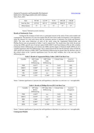
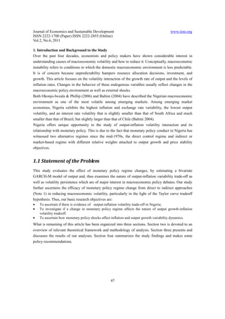
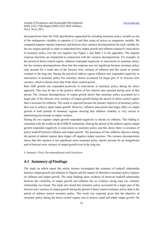
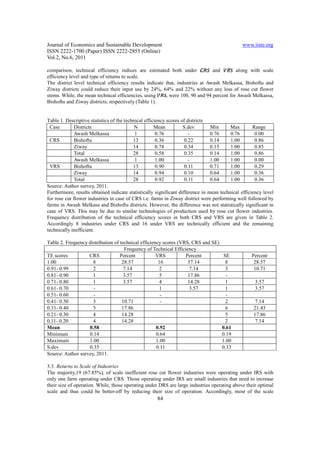
p p
Χ t = Φ 0 + ∑ Φ1i Χ t −i + Φ 2j ∑ Yt − j +ε t .......... .........1 .1
i =1 j=1

where ε t /Ω t ~ N(0, H t ) and Ω is information set available up to time t - 1
such that H t = (h yt , h πt ) ′

[ ]
Φ 0 = Φ yo , Φ π0 ′ is a 2x1 vector of constants

Χ t = [y t , π t ]′ is a 2 x 1 vector of real output growth y t and inflation rate π t .
Υ t is a vector of additional explanatory variables such as inflation uncertainty, etc
Φ 1i , Φ 2j are vectors of 2x2 matrices of parameters to be estimated.

[ ]
ε t = ε yt , ε πt ′ is a 2x1 vector of output and inflation innovations.

The vector of conditional variances of output and inflation are specified as follows:
'
H t = C0C0 + A′H t − 1 A + B ′ε t − 1ε t − 1B + D′Ft − 1D.............1.2
′
where H t = (h yt , h πt )′ is a 2x1 vectorof the conditiona variancesof output and inflation,
l
C, A, B, and D are 2x2 upper tria
ngular matricesof parameters and F is a vectorof explanator variable
; y s,
that is, F = (∆MPR, ∆Oilprices,etc).
More explicitlythe matriceof parameterscan be specifiedin upper tria ngular form as :
c c  a a  b b  δ δ 
C 0 =  11 12 ; A =  11 12 ; B =  11 12 ; and D =  11 12 .
0 c 22 
   21 22 
a a
 b 21 b 22 
  δ 21 δ 22 
 

2.2 Economic Meaning of Coefficients and Apriori Expectations
The diagonal elements in matrix Co represent the means of conditional variances of output growth and
inflation, while the off diagonal element represents their covariance. The Parameters in matrix A
depict the extents to which the current levels of conditional variances are correlated with their past
levels. In specific terms, the diagonal elements (a11 and a22) reflect the levels of persistence in the
conditional variances; a12 captures the extent to which the conditional variance of output is correlated
with the lagged conditional variance of inflation. For the existence of output-inflation volatility
trade-off, the variable is expected to have negative sign and be statistically significant. The parameters
in matrix B reveal the extents to which the conditional variances of inflation and output are correlated
with past squared innovations; b12 depicts how the conditional variance of output is correlated with the
past innovation of inflation. This measures the existence of cross-effect from an output shock to
inflation volatility. In order to estimate the impact of monetary policy on the conditional variances, we
include one period lagged change in the Central Bank’s monetary policy rate (MPR) (or VAR-based
generated monetary surprises) in the vector F. The resulting coefficients in matrix D measure the
effects of these variables on inflation and output volatility. For monetary policy to have a trade-off on
the conditional variances, the diagonal elements have to alternate in signs.
In order to address the third research question we augment the VAR model specified in (1) by adding
49

Vol.2, No.6, 2011

monetary policy variable in the vector X and then compute the generalized impulse responses and
generalized variance decompositions to analyse the short run dynamic response of output growth and
inflation monetary policy shocks/innovations. The generalized variance decomposition and impulse
response functions are unique solution and invariant to the ordering of the variables in the VAR
(Pesaran & Shin 1998). Also, it has been argued, however, that in the short run unrestricted VARs
perform better than a cointegrating VAR. For example, Naka & Tufte (1997) studied the performance
of VECMs and unrestricted VARs for impulse response analysis over the short-run and found that the
performance of the two methods is nearly identical. We adopt unrestricted VARs in attempting to
answer our third research question because of the short-term nature of the variance decomposition and
impulse response analysis. AIC and SBC will be used for lag order selection.

2.3 Method of Estimation and Data Sources
The models are estimated by the method of Broyden, Fletcher, Goldferb and Shanno (BFGS) simplex
algorithm. We employed the RATS software in the estimation of the system. This is due to the fact that
RATS has an inbuilt bivariate GARCH system that supports simultaneous estimation and thus is able
to implement different restrictions that might be assumed on the variance-covariance structure of the
system.
The data used for the estimations are quarterly data from the Central Bank of Nigeria Statistical
Bulletin of various years, the Annual Report and Statement of Account of various years.
Monetary Policy Measure: According to Nnanna (2001) the Minimum Rediscount Rate (MRR) is the
nominal anchor, which influences the level and direction of other interest rates in the domestic money
market. Its movements are generally intended to signal to market operators the monetary policy stance
of the CBN. Similarly, Agu (2007) observes that “the major policy instrument for monetary policy in
Nigeria is the minimum rediscount rate (MRR) of the Central Bank and notes that while both interest
and inflation rates are high, a worrisome problem in the observed response to these macroeconomic
imbalances is the lack of policy consistency and coherence. This could be on account of inadequate
information on the nature and size of impact of the MRR on key macroeconomic aggregates.” This
type of inconsistency in the conduct of monetary policy is likely to increase rather than stabilize
macroeconomic volatility. Hence, we shall use MRR (MPR) as a measure of monetary policy stance.

3. Presentation of Results and Discussion
Table 1 shows the summary statistics of the variables used in the study. Inflation and GDP growth
rates are calculated as annualized quarterly growth rates of consumer price index (CPI) and real GDP
respectively. As the table indicates, average nominal GDP was almost two times greater in 1995-2007
period compared to 1981-1994 period. But, the consumer price index for the period, 1995-2007, was
almost twenty fold of that in the period, 1981-1994. For this reason average real GDP for the period
1995 to 2007 was lower than that of 1981-1994.
However, the average growth rate of real GDP was higher in the second period compared to the first;
while average inflation rate for the second period was lower compared to the first period. This shows
50

Vol.2, No.6, 2011

that the economy performed better on the average under market-based monetary regime compared to
the controlled regime. The standard deviation of inflation is lower in the second period implying lower
unconditional volatility and there is no significant change in the unconditional volatility of real GDP
growth which appears to suggest that real quarterly GDP fluctuations are modest over the two periods
but slightly higher in the second period. The minimum rediscount rate, a measure of monetary policy
stance of the Central Bank of Nigeria (CBN) was on the average lower during the controlled regime
period compared to the indirect regime period. This suggests that monetary policy became tighter
during the period of indirect or market-based regime aimed specifically to control inflation by
reducing the rate of money growth.
Oil prices being used to control for exogenous shocks in the model had a low average during the
period of controlled regime. At that time lower oil prices affected GDP growth adversely as the
economy entered into a recession that led to the introduction the Structural Adjustment Programme
(SAP), which further depressed the economy. The adverse supply effect resulting from SAP and lower
oil revenue together with tighter controls on interest rate helped to put a strain on the economy. During
the period of indirect monetary approach, oil prices began to increase rapidly in the international
market and this resulted in positive output growth for most of the period and quick recovery of the
economy from the adverse effects of SAP. However, the Central Bank has been very cautious with
rising oil prices and as a result has been setting the minimum rediscount rate in order to accommodate
the adverse effects of the rise in oil prices on inflation.
Table 2 shows the tests for serial correlation, autoregressive conditional heteroskedasticity effect, and
normality. A series of Ljung-Box (1978) tests for serial correlation suggests that there is a significant
amount of serial dependence in the data. Output growth is negatively skewed, and inflation is
positively skewed and output growth failed to satisfy the Jarque-Bera tests for normality (Jarque &
Bera 1980). The ARCH tests also reveal the presence of first order serial dependence in the
conditional variances of output growth and inflation suggesting that our application of GARCH (1, 1)
model is appropriate to the data.
Valid inference from GARCH model requires that the variables be stationary, at least in their
conditional means (Lee 2002). As a result, unit root tests were conducted on the variables using the
Dickey & Fuller (1981) methodology. The analysis, however, was eventually based on the augmented
Dickey-Fuller unit root tests. The results are presented in table 3 below.
The results show that only inflation rate is level stationary while other variables are stationary in
their first differences.
Table 4 shows the results from GARCH estimations of the two sub-samples and the overall sample.
The results would help to address our concerns in the first and second research questions, which are:
whether or not the change in the approach to monetary policy in Nigeria from direct to indirect led to a
change in volatility interactions, transmissions and tradeoff between output growth and inflation. The
results are in two parts. The first part shows the estimations of the conditonal mean equation while the
second part shows the time-varying conditional variance equation which is of particular interest to us.
The first part of the conditional mean and conditonal variance eqautions represents output growth
while the second vector denotes inflation rate. The conditional mean for GDP growth shows that
51

Vol.2, No.6, 2011

inflation volatility does affect output growth negatively and this is statistically significant across the
two regimes but was highly significant during the period of indirect regime. But the effect of inflation
volatility on inflation was not certain as the cofficient was neither stable nor significant across the two
periods. Past levels of inflation are found to have positive effects on currrent inflation levels and this is
significant across the two samples while the coefficient was almost the same across the two periods.
Oil price shocks do not have any meaningful effect on inflation but do have positive and significant
effects on output growth especially in the second period. This may be due to the fact that oil price
increases which characterized most of the sample period from 1995 to 2007 may have contributed
positively to the output growth in Nigeria as a largely oil dependent economy. This result should not
be surprising as most studies have found positive output effect of oil price shocks in major
oil-exporting countries.
We are especially interested in the conditional variance equations. The estimates show that the long
run or unconditional volatilities of inflation and output growth were higher in the first period than in
the second period. The estimates for the mean covariance terms are negative and but significant only
in the first sample period. The estimates also indicate that over the sample periods, the mean
unconditional variance of output is significant across the two sample periods.
The parameters in matrix A show the extents to which the current levels of conditional variance are
correlated with their past levels. The higher estimates in the second period seem to suggest that a
current shock will have relatively long lasting effects on the future levels of the conditional variances
of output growth and inflation than it had in the first sample period. The estimates also reveal that
following change in monetary policy regime, inflation volatility and output volatility have relatively
become more persistent in Nigeria.
The off-diagonal elements in A that is A (1, 2), on the other hand, reveal the extent to which the
conditional variance of one variable is correlated with the lagged conditional variance of another
variable. The estimate for A (1, 2) appears with the expected negative sign and is statistically different
from zero for all sub-samples and the overall sample. This confirms the existence of Taylor-curve
volatility tradeoff in Nigeria. Interestingly the estimate for the sample period 1981 to 1994 is relatively
larger than the estimates for the sample period 1995 to 2007 suggesting that low inflation variability is
now associated with higher output gap variability. This seems to suggest that CBN’s efforts to stabilize
prices or specifically to target low inflation must come at a heavy cost of output fluctuations. This
result is therefore, consistent with the finding by Castelnuovo (2006) that the tighter the monetary
policy, the higher is the inflation-output gap volatility.
The parameters in B matrix reveal the extents to which the conditional variances of inflation and
output are correlated with past squared innovations (deviations from their conditional means). Of
particular interest is the off-diagonal elements B (1, 2) and B (2, 1) which depict how the conditional
variance of inflation is correlated with the past squared innovations of output. In the first sample
period there is a positive and significant volatility cross-effect from inflation to output. While in the
second period there is positive and significant volatility cross effect from output growth to inflation
variability.
In order to address the third research question we computed the impulse responses and variance
52

Vol.2, No.6, 2011

decompositions from the VAR specification augmented by including monetary policy variable as one
of the endogenous variables in equation (1.1) and then using oil prices as exogenous variable. We
computed separate impulse responses and forecast error variance decompositions for each variable for
the two regime periods in order to understand how output growth and inflation respond to innovations
in monetary policy over the two regimes (see Figure 1 and Table 5 in the appendix). The impulse
response functions are interpreted in conjunction with the variance decompositions. For example, in
the period of direct control regime, inflation responded negatively to innovations in monetary policy
but the variance decompositions show that this response was not significant because monetary policy
only account for a small part of the forecast error variance of inflation and this seems to remain
constant in the long run. During the period of indirect regime inflation also responded negatively to
innovations to monetary policy but monetary shocks accounted for larger part of its forecast error
variance, which is almost twice that of the direct control period.
Real GDP growth rate responded positively to innovations in monetary policy during the direct
approach. This may be due to the positive effects of low interest rates pursued during most of that
period. The variance decomposition of output growth shows that monetary policy accounted for a
larger part of the forecast error variance of output growth during the period of direct control regime
than it accounts for inflation. This result is expected because the primary objective of monetary policy
then was to achieve rapid output growth. However, inflation innovations had larger effect on output
growth in both periods of monetary regimes showing that inflation volatility is very crucial in
determining movements in output variance.
During the two regimes output growth responded negatively to shocks on inflation. This finding is
consistent with the results in the GARCH estimations. During the period of the indirect regime output
growth responded negatively to innovations to monetary policy and this shows there is existence of
policy tradeoff between inflation and output growth. The pursuance of low inflation objective during
the period of indirect regime does trigger off negative output reactions. The variance decomposition
shows that this reaction is not significant since monetary policy shocks account for an insignificant
part of forecast error variance of output growth even in the long run.

4. Summary, Policy Recommendations and Conclusion

4.1 Summary of Findings
The study on which report this article focuses investigated the existence of tradeoff relationship
between output growth and inflation in Nigeria and the impact of alternative monetary policy regimes
on inflation and output growth. The study findings show evidence of short-run tradeoff relationship
between the variability of output growth and inflation but no evidence strong long run volatility
relationship was found. The study also found that monetary policy accounted for a larger part of the
forecast error variance of output growth during the period of direct control monetary policy than in the
period of indirect control monetary policy. This result was expected given that the objective of
monetary policy during the direct control regime was to achieve rapid and stable output growth. On
53

Vol.2, No.6, 2011

the other hand, the response of inflation to monetary policy changes in the period of indirect or
market-based regime was larger compared to its response during the period of direct control. Again,
this result is not surprising because the major focus of monetary policy in Nigeria during the period of
indirect control was to achieve low inflation.
The results of the study further reveal that the volatility of output growth and inflation during the
period of market-based policy regime are more persistent compared to the period of direct controls.
Evidence of volatility cross-effect from output to inflation and vice versa was present but not
significant across the two sample periods. The results fail to establish clearly any evidence to suggest
that monetary policy tradeoff is a long run phenomenon. From these findings, the following policy
recommendations could be made.

4.2 Policy Recommendations
Market-based or indirect control approach to monetary policy conduct in Nigeria should be carefully
examined regularly in order to ascertain its desirability and workability. This would help to determine
when changes in monetary policy stance actually affect the variability of output and inflation and in
what direction. Policy makers should be careful not to believe too fervently that the market works in
Nigeria. Policy changes could trigger off more volatility than demand or supply shocks. This reflects
the fact that market imperfection is very typical of developing countries with underdeveloped financial
markets. In Nigeria, it is hard to believe that inflation is caused by excessive money growth or the
growth of credit. Instead, inflation has been driven largely by high cost of doing business, rising cost
of energy prices and depreciating exchange rate that has made the cost of imported raw materials
exceedingly high. This has intensified the effect of adverse supply shocks on inflation. Again, the size
of the informal and non-monetized sector of the economy is quite substantial making it possible for
monetary policy to have a big impact. In such a macroeconomic environment, tightening of monetary
policy in response to high inflation would exacerbate an already heated environment by increasing the
cost of credit to firms that depend on borrowing as the major source of finance.
Our study reveals that volatility tradeoff is higher during the period of indirect monetary regime than
during the period of direct control and that output is responding negatively to monetary shocks. This
implies that the Central Bank should be very cautious of the objective of targeting low inflation as
such a policy could trigger off not only low output growth but also high output growth volatility.
Finally, we suggest that monetary policy instruments be supported by other fiscal and physical
measures such as ensuring that energy cost, the cost of imported raw materials and possibly the cost of
housing are reduced through other improved supply-side processes. While, attention is being focus on
low inflation it is also pertinent to realize that high and stable output growth objective is equally
important to Nigeria as a developing economy. There should be a balance between output growth
objective and low inflation. The study reveals that monetary policy objective that targets low inflation
would be likely achieved at a heavy cost in terms of adverse output growth effect.

54

Vol.2, No.6, 2011

4.3 Conclusion
This study has shown that there is very little empirical evidence to suggest that monetary policy
regime change necessarily alters existing inflation-output growth variability tradeoff. It could not find
strong evidence of long run tradeoff between output growth and inflation, which is required in order to
ascertain the effectiveness of monetary policy regime changes from that perspective. This is not
altogether surprising as half of the studies undertaken on this same issue in other jurisdictions have
thus far found no evidence of long run policy tradeoff (see Lee 2004 for example). However, most
studies did find that volatility tradeoff changed when monetary policy regime changed, this study
seems to corroborate the same findings. It is perhaps important to observe here that the availability of
good quality macroeconomic data at short-time intervals like monthly or quarterly series remains a
major challenge to policy-relevant research in Nigeria. However, the situation is not very much
different in most other developing countries. Using extrapolated quarterly GDP data in empirical
studies of this nature may influence the research outcomes since such data were econometrically
generated under certain assumptions. Further research is therefore recommended in this issue in the
future, particularly as high frequency and good quality data begin to be available. It would indeed be
very informative to policy makers in Nigeria who are currently experimenting with the adoption of
inflation targeting monetary policy regime to read this research output. It will perhaps assist them in
appreciating the cost of such regime in terms of output growth volatility.

References
Agu, C. (2007). What Does the Central Bank of Nigeria Target: An Analysis of Monetary Policy
Reaction Function in Nigeria. African Economic Research Consortium (AERC), Nairobi, Kenya.
Baltini, N. (2004). Achieving and Maintaining Price Stability in Nigeria. IMF Working Paper,
WP/04/97.
Castelnuovo, E. (2006). “Monetary Policy Switch, the Taylor Curve and Great Moderation”, [Online]
Available: http://ssrn.com/abstract=880061].
Dickey, D. A., & Fuller, W. A. (1981). Likelihood Ratio Statistics for Autoregressive Time Series with
a Unit Root. Econometrica, 49, 1057–1072.
Fountas, S., Menelaos, K. & J. Kim (2002). Inflation and Output Growth Uncertainty and their
Relationship with Inflation and Output Growth. Economics Letters, 75, 293-301.
Fountas, S. & Menelaos, K. (2007). Inflation, Output Growth, and Nominal and Real Uncertainty:
Empirical Evidence for the G7. Journal of International Money and Finance, 26, 229-250.
Fuhrer, J. (1997). Inflation/Output Variance Trade-offs and Optimal Monetary Policy. Journal of
Money, Credit and Banking, 29(2), 214-34.
Gaspar, V. & Smets, F. (2002). Monetary Policy, Price Stability and Output Gap Stabilization.
International Finance, 5(2), 193-211.
Grier, K. B., Henry, O. T., Olekalns, N. & Shields, K. (2004). The Asymmetric Effects of Uncertainty
55

Vol.2, No.6, 2011

on Inflation and Output Growth. Journal of Applied econometrics, 19, 551–565.
Jarque, C. M. & Bera, A. K. (1980). Efficient tests for normality, homoscedasticity and serial
independence of regression residuals. Economics Letters, 6, 255–259.
Lee, J. (2002). The Inflation-Output Variability Tradeoff and Monetary Policy: Evidence from a
GARCH Model. Southern Economic Journal, 69(1), 175-188.
Lee, J. (2004). The Inflation-Output Variability Tradeoff: OECD Evidence. Journal of Contemporary
Economic Policy, 22(3), 344-356.
Ljung, G. M. & Box, G. E. P. (1978). On a Measure of Lack of Fit in Time Series Models. Boimetrika,
66: 66–72.
Naka, A. & Tufte, D. (1997), Examining the Impulse Response Functions in Cointegrated Systems;
Applied Economics, 29, 1593-1603.
Nnanna, O. (2001). Monetary Policy Framework in Africa: the Nigerian Experience. Central Bank of
Nigeria, Working Paper.
Okonjo-Iweala, N. & Philip Osafo-Kwaako. (2006). Nigeria’s Economic Reforms: Progress and
Challenges. Brookings Global Economy and Development, Working Paper, 6, 1-30.
Pesaran, M. H. and Y. Shin (1998). Generalised impulse response analysis in linear multivariate
models. Economic Letters, 58 , 17-29.
Roberts, J. M. (2006). Monetary Policy and Inflation Dynamics. International Journal of Central
Banking, September, 2006.
Taylor, J. (1979). Estimation and control of Macroeconomic Model with Rational Expectations.
Econometrica, 47(5), 1267-86.
Taylor, J. (1994). The Inflation/Output Variability Trade-off Revisited, in Goals, Guidelines and
Constraints Facing Monetary Policymakers. FRB of Boston, Conference Series 38, 21-38.

Notes
Note 1. Other studies failed to distinguish the two periods in their analyses and thus evaluate the
effectiveness of the CBN’s monetary policy even over the period when monetary policy in Nigeria had
overbearing political interference.
Note 2. Gaspar, Victor and Frank Smets (2002) “Monetary Policy, Price Stability and Output Gap
Stabilization.” International Finance, 5:2, 193-211

Figures
Impulse Response Functions

56

Vol.2, No.6, 2011

Plot of responses of inflation rate 1981-1994
0.08

0.06

0.04

0.02

0.00

-0.02

-0.04

-0.06

-0.08
0 1 2 3 4 5 6 7 8 9 10 11 12 13 14 15 16 17 18 19 20 21 22 23
Real GDP Growth Rate 1981-1994 MRR 1981-1994 inflation rate 1981-1994

Figure 1. Plot of responses of inflation rate 1981-1994

Plot of responses of MRR 1981-1994
10

8

6

4

2

0

-2

-4
0 1 2 3 4 5 6 7 8 9 10 11 12 13 14 15 16 17 18 19 20 21 22 23

Figure 2. Plot of responses of MRR 1981-1994

Plot of responses of Real GDP Growth Rate 1981-1994
2.5

2.0

1.5

1.0

0.5

0.0

-0.5
0 1 2 3 4 5 6 7 8 9 10 11 12 13 14 15 16 17 18 19 20 21 22 23

Figure 3. Plot of responses of Real GDP Growth Rate 1981-1994

57

Vol.2, No.6, 2011

Plot of responses of inflation rate 1995-2007
0.050

0.025

-0.000

-0.025

-0.050

-0.075

-0.100

-0.125
0 1 2 3 4 5 6 7 8 9 10 11 12 13 14 15 16 17 18 19 20 21 22 23

Figure 4. Plot of responses of inflation rate 1995-2007

Plot of responses of MRR 1995-2007
14

12

10

8

6

4

2

0

-2

-4
0 1 2 3 4 5 6 7 8 9 10 11 12 13 14 15 16 17 18 19 20 21 22 23

Figure 5. Plot of responses of MRR 1995-2007

58

Vol.2, No.6, 2011

2.5
2.0
1.5
1.0
0.5
0.0
-0.5
-1.0
-1.5
0 5 10 15 20
Real GDP Growth Rate 1995-2007 inflation rate 1995-2007
MRR 1995-2007

Figure 6. Plot of responses of Real GDP Growth Rate 1995-2007

Tables
Table 1. Summary Statistics of Study Variables
Series Sample obs mean Std Dev Minimum Maximum
GDP 1981:1 2007:1 108 409541.01 220926.82 205045 1317391.3
1981:1 1994:4 56 283126.25 44004.84 205045 347271.1
1995:1 2007:4 52 545679.97 252724.21 348746.7 1317391.3
CPI 1981:1 2007:1 108 2459.17 2697.68 47.9 8722.6
1981:1 1994:4 56 291.44 320.28 47.9 1458.4
1995:1 2007:4 52 4793.65 2107.46 1669.9 8722.6
INFLAcbn 1981:1 2007:1 108 23.66 19.91 1.3 77.9
1981:1 1994:4 56 27.77 19.89 3.0 66.7
1995:1 2007:4 52 19.23 19.14 1.3 77.9
Oilprices 1981:1 2007:1 108 28.07 15.23 11.4 90.7
1981:1 1994:4 56 23.56 6.94 13.6 38
1995:1 2007:4 52 32.94 19.71 11.4 90.7
Mrr 1981:1 2007:1 108 14.07 4.41 6 26
1981:1 1994:4 56 13.28 5.24 6 26
1995:1 2007:4 52 14.93 3.12 8 20
LOGRGDP 1981:1 2007:1 108 10.7 1.43 9.0 14.1
1981:1 1994:4 56 11.94 0.81 10.1 13.1
1995:1 2007:4 52 9.35 0.20 9.0 10.0
GDPGRT 1981:1 2007:1 107 0.54 1.1 -1.1 6.8
1981:1 1994:4 55 0.31 1.02 -1.1 6.8
59

Vol.2, No.6, 2011

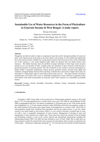
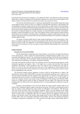
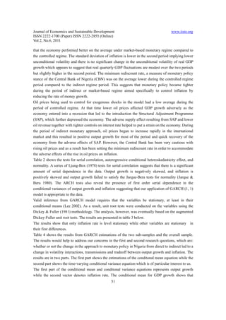
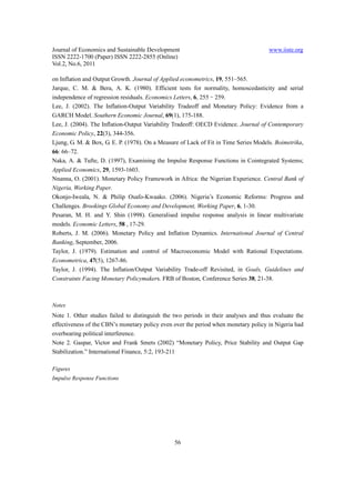
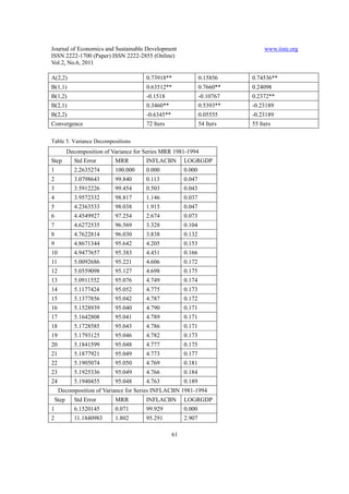
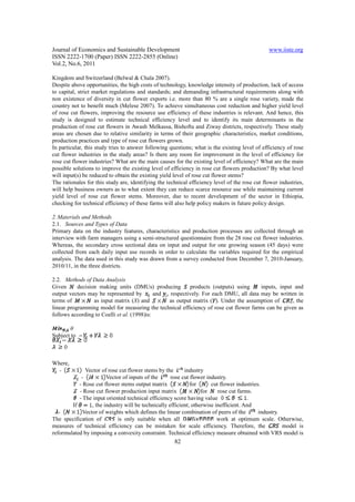
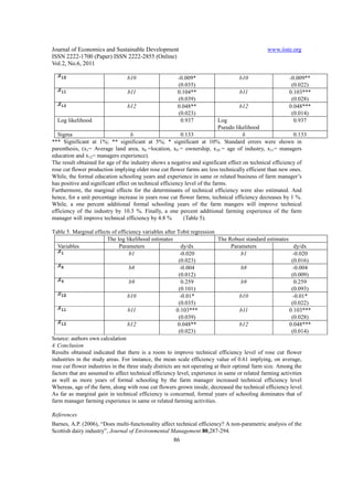
1995:1 2007:4 52 0.77 1.1 -0.6 4.6

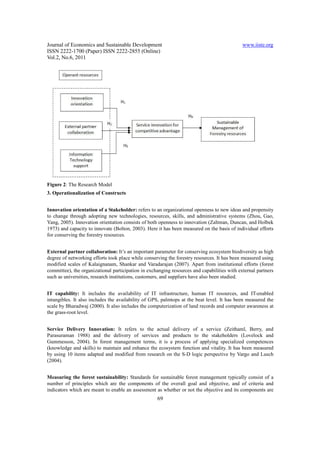
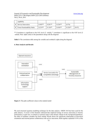
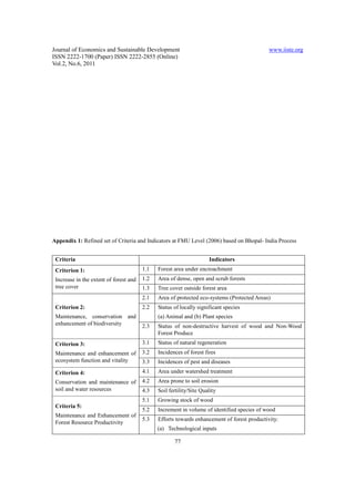
Table 2. Tests for Serial Correlation, ARCH and Normality
Tests for Serial Correlation, ARCH and Normality
Series Q(8) Q(16) Q(24) ARCH(1) ARCH(2) JB-STAT
GDPGRWT 21.778[0.0006] 54.765[0.000] 82.40[0.000] 16.636[0.000] 5.846[0.00537] 2.228[0.3283]
INFLACBN 65.281[0.0000] 76.992[0.000] 82.846[0.00] 11.787[0.006] 40.51[0.0000] 21.037[0.07]

Table 3. Unit Root Tests of Variables of the Model
Variable Level First Difference Lags
Logrgdp -3.139162* -3.755954** 1
Inflacbn -2.450268** -3.935362** 1
Oilprices 1.576064 -4.293117** 1
Logoilprices -0.001255 -4.789354** 1
MRR -2.890303 -5.668382** 1
GDPGRT -2.385600 -7.695887** 3

Table 4. Bivariate GARCH Estimations of Output Growth and Inflation
BIVARIATE GARCH ESTIMATIONS OF OUTPUT GROWTH AND INFLATION
CONDTIONAL MEAN EQUATIONS
1981:1 2007:4 1981:1 1994:4 1995:1 2007:4
Variables Mod1 Mod11 Mod21
CONSTANT -7.51810** -5.546* -3.43389
Trend 0.07571** -0.011 0.021079
GRGDP{1} 0.05173 0.073 -0.1475
INFLA_VOL -0.09100** -0.0897* -0.1000**
OILP_SHOCK 3.98553** 6.7809 6.3037**
CONSTANT 7.65128** 10.3289** -0.1001
Trend -0.07907** -0.10556 0.009257
INFLACBN{1} 0.70064** 0.7497** 0.70817**
INFLA_VOL 0.2668** 0.28209 -0.10738
OILP_SHOCK 0.05470 -18.9548** 0.10766
CONDITIONAL VARIANCE EQUATIONS
C(1,1) 2.55319** 4.4927** 3.7733**
C(1,2) -0.51521 -4.57815** -0.4757
C(2,2) 1.9726** 0.7345 0.000055
A(1,1) 0.9095** 0.1876 0.87385**
A(1,2) -0.41810** -1.0158** -0.37536**

60

Vol.2, No.6, 2011

A(2,2) 0.73918** 0.15856 0.74536**
B(1,1) 0.63512** 0.7660** 0.24098
B(1,2) -0.1518 -0.10767 0.2372**
B(2,1) 0.3460** 0.5393** -0.23189
B(2,2) -0.6345** 0.05555 -0.23189
Convergence 72 Iters 54 Iters 55 Iters

Table 5. Variance Decompositions
Decomposition of Variance for Series MRR 1981-1994
Step Std Error MRR INFLACBN LOGRGDP
1 2.2635274 100.000 0.000 0.000
2 3.0798643 99.840 0.113 0.047
3 3.5912226 99.454 0.503 0.043
4 3.9572332 98.817 1.146 0.037
5 4.2363533 98.038 1.915 0.047
6 4.4549927 97.254 2.674 0.073
7 4.6272535 96.569 3.328 0.104
8 4.7622814 96.030 3.838 0.132
9 4.8671344 95.642 4.205 0.153
10 4.9477657 95.383 4.451 0.166
11 5.0092686 95.221 4.606 0.172
12 5.0559098 95.127 4.698 0.175
13 5.0911552 95.076 4.749 0.174
14 5.1177424 95.052 4.775 0.173
15 5.1377856 95.042 4.787 0.172
16 5.1528939 95.040 4.790 0.171
17 5.1642808 95.041 4.789 0.171
18 5.1728585 95.043 4.786 0.171
19 5.1793125 95.046 4.782 0.173
20 5.1841599 95.048 4.777 0.175
21 5.1877921 95.049 4.773 0.177
22 5.1905074 95.050 4.769 0.181
23 5.1925336 95.049 4.766 0.184
24 5.1940455 95.048 4.763 0.189
Decomposition of Variance for Series INFLACBN 1981-1994
1 6.1520145 0.071 99.929 0.000
2 11.1840983 1.802 95.291 2.907

61

Vol.2, No.6, 2011

3 15.0407379 3.934 91.002 5.063
4 17.5910999 5.983 87.708 6.308
5 19.0795657 7.843 85.209 6.949
6 19.8504330 9.436 83.355 7.209
7 20.2077581 10.698 82.044 7.258
8 20.3628070 11.607 81.174 7.220
9 20.4350821 12.201 80.627 7.172
10 20.4786903 12.556 80.296 7.149
11 20.5120032 12.752 80.092 7.155
12 20.5388952 12.857 79.962 7.182
13 20.5596652 12.911 79.872 7.217
14 20.5748203 12.941 79.807 7.252
15 20.5855134 12.958 79.758 7.285
16 20.5930675 12.967 79.719 7.313
17 20.5985954 12.972 79.689 7.338
18 20.6028938 12.975 79.665 7.360
19 20.6064990 12.975 79.645 7.380
20 20.6097764 12.973 79.627 7.400
21 20.6129850 12.970 79.611 7.420
22 20.6163087 12.966 79.595 7.439
23 20.6198692 12.961 79.580 7.459
24 20.6237341 12.957 79.564 7.480
Decomposition of Variance for Series LOGRGDP 1981-1994
1 0.0606513 2.224 35.541 62.235
2 0.1051127 4.838 41.180 53.982
3 0.1455233 6.553 43.994 49.453
4 0.1817223 7.954 45.165 46.882
5 0.2136589 9.201 45.422 45.376
6 0.2416622 10.339 45.191 44.470
7 0.2662894 11.377 44.717 43.906
8 0.2881627 12.320 44.145 43.535
9 0.3078669 13.172 43.556 43.272
10 0.3258997 13.937 42.997 43.066
11 0.3426582 14.624 42.488 42.888
12 0.3584433 15.240 42.039 42.722
13 0.3734729 15.793 41.647 42.559
14 0.3878983 16.293 41.310 42.398

62

Vol.2, No.6, 2011

15 0.4018202 16.745 41.019 42.236
16 0.4153033 17.157 40.767 42.076
17 0.4283879 17.534 40.548 41.918
18 0.4410995 17.880 40.355 41.765
19 0.4534554 18.201 40.183 41.616
20 0.4654687 18.498 40.028 41.474
21 0.4771516 18.774 39.887 41.338
22 0.4885159 19.032 39.758 41.210
23 0.4995741 19.273 39.639 41.088
24 0.5103391 19.499 39.529 40.973
Decomposition of Variance for Series MRR 1995-2007
1 1.1350644 100.000 0.000 0.000
2 1.6579561 98.990 0.634 0.376
3 1.9518658 98.041 1.594 0.365
4 2.1059278 97.576 2.035 0.389
5 2.1890956 97.572 1.940 0.488
6 2.2471307 97.176 2.068 0.757
7 2.3094247 95.447 3.279 1.275
8 2.3891806 92.145 5.816 2.039
9 2.4856879 87.850 9.202 2.949
10 2.5901409 83.418 12.706 3.876
11 2.6920664 79.478 15.792 4.730
12 2.7834456 76.298 18.235 5.467
13 2.8600548 73.886 20.033 6.081
14 2.9210218 72.125 21.291 6.584
15 2.9676945 70.865 22.140 6.995
16 3.0025083 69.967 22.701 7.332
17 3.0281459 69.320 23.069 7.611
18 3.0470430 68.841 23.314 7.845
19 3.0611754 68.473 23.482 8.045
20 3.0720291 68.178 23.603 8.219
21 3.0806628 67.931 23.695 8.374
22 3.0878022 67.716 23.771 8.514
23 3.0939296 67.522 23.836 8.642
24 3.0993574 67.344 23.894 8.762
Decomposition of Variance for Series INFLACBN 1995-2007

63

Vol.2, No.6, 2011

1 2.6954031 5.347 94.653 0.000
2 5.4978721 7.572 89.068 3.360
3 8.1216124 11.195 84.123 4.682
4 10.2911556 14.430 80.076 5.494
5 11.9097715 17.231 76.848 5.921
6 13.0111184 19.547 74.326 6.127
7 13.6946354 21.374 72.430 6.196
8 14.0795505 22.727 71.083 6.191
9 14.2745317 23.651 70.196 6.153
10 14.3626479 24.223 69.665 6.113
11 14.3984216 24.535 69.380 6.085
12 14.4124976 24.679 69.246 6.075
13 14.4192880 24.730 69.190 6.080
14 14.4241316 24.737 69.168 6.095
15 14.4283203 24.729 69.157 6.114
16 14.4318686 24.718 69.149 6.133
17 14.4346655 24.708 69.140 6.152
18 14.4367583 24.701 69.131 6.167
19 14.4383088 24.696 69.123 6.181
20 14.4394976 24.692 69.116 6.193
21 14.4404705 24.689 69.109 6.203
22 14.4413283 24.686 69.102 6.212
23 14.4421380 24.683 69.097 6.221
24 14.4429453 24.680 69.091 6.229

64

Vol.2, No.6, 2011

New approaches to sustainable forest management: a study of
service innovation in conserving forestry resources
Verma Rajeev (corresponding author)
Fellow Participant in Management
Indian Institute of Management, Indore, India
Email: f09rajeev@iimidr.ac.in


The author would like to thank Prof. P C Kotwal, Indian Institute of Forest Management, Project
Coordinator, IIFM –ITTO Project and Forest MIS of Chhattisgarh Forest Department, to operationalize this
study.

Abstract
Sustainability has been a primary concern for the forestry professionals. This paper is concerned with the
continuing evolution of approaches to monitor sustainable forest management. It summarises the existing
knowledge base and primary techniques and strategies for achieving socially and environmentally
acceptable SFM in various forest formations. Service innovation is one means for the improved
monitoring of SFM through the introduction of scientifically based criteria and indicators. This set has been
developed on the basis of Dry Forest Asia Initiative. In addition, their implementation has played a key role
in interactions with local beneficiaries. Yet, research on the link between service innovation and natural
resource management is scant. The paper identifies innovation orientation, external partner collaboration,
and information capability as operant resources along with the operand resources captured under the 8
criteria and their respective field level indicators. These antecedents are analyzed to know impact of overall
service innovation on social economic development of the area.

Keywords: sustainable forest management, service innovation, C&I, community participation

1. Introduction

The United Nations Conference on Environment and Development (UNCED) in 1992 led the general
adoption of a concept of sustainable development based on the equilibrium between three prime
components i.e., economic development; conservation of the environment and social justice. Forestry
resources have been featured prominently at the conference and have remained high on the international
agenda for sustainable development. In pursuance of the ‘Forest Principles’ and of Agenda 21 (chapter 11)
adopted at UNCED, the notion of sustainable forest management has been adopted in more specific and
operational terms. Criteria and indicators were identified in order of planning, monitoring and assess the
forest management practices at the national as well as for the individual forest management unit (FMU)
level. The selection and use of suitable criteria and indicators are thus one of the keys to progress in the
practice of sustainable forest management.

65

Vol.2, No.6, 2011

These criteria and indicators are mainly intended for defining objectives and priorities for Sustainable Forest
Management (SFM) and for monitoring progress during their implementation. The objective of SFM is, to
increase the adoption of forest management practices to sustain and enhance the yields of multiple products,
services and values for multiple stakeholders, over the long term. However, the intermediate goal is to
contribute, sustain and enhance the benefits from natural tropical forests like India, by increasing
opportunities and benefits to various stakeholders. The end benefit of the project includes rural livelihood
promotion; industrial timber production; and environmental services. In a way, improving the level of
adoption of scientific findings in forest management, leads to adoptive management process and hence use of
best practices. In India, all the forestry resources are under the direct control of the government. Hence, it
provides a very less scope for the innovative management. However, the latest management practices such
as, Sustainable Forest Management (SFM), Joint Forest Management (JFM) bring the inputs from various
stake holders and a hope to bring the service innovation in the management of the forestry resources.

These service innovations in the management of natural resources have been an effective way for the
forestry organizations to accelerate its growth rate and profitability as products or services become more or
less homogeneous or an original competitive advantage cannot be sustained (Berry, Shankar, Janet, Susan
and Dotzel, 2006). Accordingly, researchers and practitioners are interested in explaining and predicting
key antecedents of and outcomes associated with service innovation in managing forestry resources. Much
of the research on service innovation in the last few decades has addressed many considerations,
including decisions of service innovation adoption (Frambach, Barkema, Bart and Wedel, 1998; Kleijnen,
Ruyter, and Andreassen 2005), typologies (Avlonitis, Papastathopoulou, and Gounaris 2001) of service
innovation, service innovation strategy and process (Blazevic and Lievens 2004), and drivers of service
innovation (Berry et al. 2006) mainly in the corporate scenario of the western countries. However, the
present work focuses on the importance of innovation practices in conserving forestry resources and
highlights the need of future research in this area. By shedding light on the short and long-term benefits and
different goods/ services for different stakeholders, this forest management practice contributes both to the
environment as well as to its various stakeholders.

As suggested by Berry et al. (2006), service innovation aims to create new markets and hence possibilities
of extending the organizational service reach. Research seeks to contribute to sustainable forest
management by increasing the understanding of the costs and benefits for different stakeholders of
sustaining or replacing, managing well or degrading natural forests, by enhancing the incentives for
improved forest management through contributions for institutional development and policy decisions; and
by evaluating harvesting and management recommendations to sustain commodities and environmental
values from natural tropical forests.

However, this topic has recently attracted increasing interest from academics and practitioners (e.g., Blind
2006; Dean 2004; Pavlovski 2007; Verganti and Buganza 2005; Zomerdijk and de Vries 2007), there is little
evidence of significant innovation in managing forestry resources. We argue that there is no full and
adequate understanding of the concept of service innovation and its role in managing forestry resources.
Recently, the field of marketing has evolved toward a service-dominant (S-D) logic (Vargo and Lusch 2008)
through which we can re-examine the role of innovation in service delivery. Compared to traditional
goods-dominant (G-D) logic, service in S-D logic is the application of specialized competences (knowledge
and skills, i.e., operant resources) to provide through goods (operand resources) that benefit an entity.

In the present article, we argue that service innovation is the process of applying specialized competences,
consistent with S-D logic. Innovation in this context is the process of applying new ideas or current
thinking in fundamentally different ways, resulting in significant changes. According to S-D logic,
66

Vol.2, No.6, 2011

innovations had significantly changed the user preferences and their perception about the service quality
(Madhavaram and Hunt, 2008). Therefore, by implementing innovative practices in service delivery,
organizations could change their method of creating stakeholders value and hence positively impact their
perceptions. Accordingly, we argue that service delivery innovation in the SFM context, involves an entire
organization viewing and addressing both value creation and environmental services within an S-D logic
framework.

The purpose of this article is to contribute to the literature on Sustainable Forest Management through
service delivery innovation by developing and empirically testing a model that attempts to explain what
motivates service delivery innovation and, in turn, influences performance in terms of optimum utilization
of forestry resources. Here the performance has been measured on the basis of Bhopal-India initiative for
SFM, which in itself is an outcome of Dry Forest Asia Initiative. We had three research objectives: (a) to
understand the role of service innovation in SFM (b) to investigate the antecedents of service delivery
innovation based on the Local Unit Criteria and Indicator Development (LUCID) for SFM, and (c) to
examine whether proposed service innovation can result in better social economic development in terms of
rural livelihood promotion.

This article makes three contributions to the literature. First, we try to identify the nature of service delivery
innovation in the management of natural resources. By studying innovation within the framework of S-D
logic, we view service delivery innovation as ability of a firm to create stakeholder value (Lievens and
Moenaert, 2000). Second, based on resource advantage (R-A) theory (Lusch, Vargo and Brien, 2007), we
test the links among organizational innovation orientation, service delivery innovation, and performance
through an empirical survey with samples from 126 JFMC’s. Third, the results provide practical steps for
managers to understand service innovation that can result in better social economic development in terms of
rural livelihood promotion. The article is structured as follows. First, we review Sustainable Forest
Management in terms of S-D logic framework to identify the key operant resources that facilitate service
delivery innovation. Then, after describing the research framework (Figure 1), we report the results of a
study conducted in the Forest Management Committees aimed at empirically testing the research model
(Figure 2). At last, we conclude with a discussion of theoretical and managerial implications and directions
for future research.

2. Theoretical Background and Conceptual Framework

Looking into the service innovation literature, most of the prior innovation literature has treated service
innovation as product innovation. However, extensive literature review includes the interaction (i.e.,
co-production with end users) between new service development and service delivery (Zaltman, Duncan
and Holbek, 1973). Although strategic innovation theory (Markides, 1997) addresses a new way of
delivering new products or services to existing or new customer segments and most adequately explains
service innovation, it focuses mainly on goods (i.e., operand resources) but not on operant resources.

As we know, R-A theory is compatible with the S-D logic’s emphasis on competences, value propositions,
and operant resources. In this study, we view service delivery innovation from the R-A theory to better
understand the relationships among strategic and organizational issues. R-A theory is a process theory of
competition, which asserts that firms achieve superior financial performance by occupying marketplace
positions of competitive advantage. Here in terms of forest management, the competency may be achieved
in terms of optimum utilization of forestry resources, socio-cultural benefits and better ecosystem function
and vitality.

67

Vol.2, No.6, 2011

Hence it relies on those resources that provide the firm a comparative advantage over its competitors. These
comparative resources, in the S-D logic perspective, are mainly operant resources. Figure 1 presents our
research framework.

Figure 1: The Research Framework

Operant resources that can be leveraged to develop innovation practices, a source of sustained competitive
advantage, produce superior performance in terms of improved sustainability indicators. Further, we are
also suggesting a direct effect between innovation practices on sustainability of forestry resources. In our
discussion, we refer to the concept of applying R-A theory to support service delivery innovation research.
To determine which operant resources facilitate service delivery innovation, however, one needs a model
describing the resources/capabilities of a firm and how these enable service delivery innovation. The model
has been based on the study Verganti and Buganza (2005) that describes service delivery as being facilitated
by organization (internal and external) and technology. We therefore propose a research model and suggest
that innovation practices in service delivery are mainly influenced by organizational, relational, and
informational resources (Hunt 2000). In R-A theory, organizational (e.g., cultures), relational (e.g.,
relationships with partners), and informational (e.g., technology) assets are operant resources.

We further identify organizational resources as innovation orientation, relational resources as external
partner collaboration, and informational resources as IT capabilities. The emphasis in the literature is the
discussion of organization, relationships, and technology and their influence on service delivery innovation
and monitoring of sustainable management of forestry resources. It shows the relationships that we
hypothesized exist among innovation orientation, external partner collaboration, IT capability, service
delivery innovation, and performance of sustainability indicators.

68

Vol.2, No.6, 2011

Figure 2: The Research Model
3. Operationalization of Constructs

Innovation orientation of a Stakeholder: refers to an organizational openness to new ideas and propensity
to change through adopting new technologies, resources, skills, and administrative systems (Zhou, Gao,
Yang, 2005). Innovation orientation consists of both openness to innovation (Zaltman, Duncan, and Holbek
1973) and capacity to innovate (Bolton, 2003). Here it has been measured on the basis of individual efforts
for conserving the forestry resources.

External partner collaboration: It’s an important parameter for conserving ecosystem biodiversity as high
degree of networking efforts took place while conserving the forestry resources. It has been measured using
modified scales of Kalaignanam, Shankar and Varadarajan (2007). Apart from institutional efforts (forest
committee), the organizational participation in exchanging resources and capabilities with external partners
such as universities, research institutions, customers, and suppliers have also been studied.

IT capability: It includes the availability of IT infrastructure, human IT resources, and IT-enabled
intangibles. It also includes the availability of GPS, palmtops at the beat level. It has been measured the
scale by Bharadwaj (2000). It also includes the computerization of land records and computer awareness at
the grass-root level.

Service Delivery Innovation: It refers to the actual delivery of a service (Zeithaml, Berry, and
Parasuraman 1988) and the delivery of services and products to the stakeholders (Lovelock and
Gummesson, 2004). In forest management terms, it is a process of applying specialized competences
(knowledge and skills) to maintain and enhance the ecosystem function and vitality. It has been measured
by using 10 items adapted and modified from research on the S-D logic perspective by Vargo and Lusch
(2004).

Measuring the forest sustainability: Standards for sustainable forest management typically consist of a
number of principles which are the components of the overall goal and objective, and of criteria and
indicators which are meant to enable an assessment as whether or not the objective and its components are
69

Vol.2, No.6, 2011

being accomplished. In the present study, criteria have been formulated to describe a desired state or
dynamics of the biological or social system and allow a verdict on the degree of achievement of an
objective in a given situation. A scale consists of 8 criteria and 44 indicators have been used to monitor the
forest sustainability at the National Level.

4. Hypothesis Development

In a study conducted by Zhou et al, (2005) the innovation orientation has been determined as one of the
factors for service innovation. It has been noted as a key driver for overcoming hurdles and enhancing
organizational ability to successfully adopt or implement new systems, processes, or products. In case of
conserving forestry resources, it comes in the form of individual efforts to maintain the forest resource
productivity. Therefore, innovation orientation represents the extent to which (a) an organization is open to
new ideas (i.e., culture) through the adoption of new technologies and integrated resources and (b)
encouragement of forest management committee members to consider the adoption of innovation. Hence,
we propose that the organizational ability to adapt to changing or existing service depends upon innovation
orientation of its individual members. We formulate the following hypothesis:

Hypothesis 1: Innovation orientation of individual JFMC members has a positive impact on service
innovation in forest conservation scenario at 95 percent confidence level.

The Inter-organizational collaboration is important in supplementing the internal innovative activities of
organizations (Deeds and Rothaermel 2003). Therefore, firms need to collaborate to build greater
innovation practices and lock-in partners for the long term. Due to this firms may improve their ability to
engage in process innovation by managing their relationships with suppliers and customers (Kaufman,
Wood, and Theyel 2000). Therefore, we propose that innovative service delivery that a firm creates is based
on support from external partners’ collaboration (e.g., stakeholders, research institutions, and universities).
Hence, we propose that firms having stronger collaborations with external partners will be better at
developing new methods (approaches) of service innovation for conservation of natural resources.
Therefore, we hypothesize the following:

Hypothesis 2: External partner collaboration has a positive impact on service innovation in forest
conservation scenario at 95 percent confidence level.

Based on the study on operant resources that bundle basic resources (Hunt 2000), we propose that IT
capability is a hierarchy of composite operant resources (COR) that includes IT infrastructure, human IT
resources, and IT-enabled intangibles. Technology may influence organizational ability to create value that
will transform the way customers interact with an offering. To create a new channel or method of service
delivery, organization needs to possess this infrastructure. In terms of managing the sustainable resources, it
comes in the form of latest GPS supported infrastructure; Satellite based forest fire fighting equipments etc.
Thus, IT capability is the operant resource for a new service that offers an opportunity to provide new and
innovative services. We hypothesize the following:

Hypothesis 3: IT capability has a positive impact on service innovation in forest conservation scenario at
95 percent confidence level.

Prior research has studied business performance from different perspectives, such as financial performance,

70

Vol.2, No.6, 2011

business unit performance, or organizational performance (Wiertz, Ruyter, Keen and Streukens, 1986).
Based on R-A theory, once competitors achieve superior performance through obtaining marketplace
positions of competitive advantage, firms attempt to leverage the advantages through major innovation
practices. We therefore propose that if organization is able to innovate in more varied ways to deliver
service, they will achieve superior performance objectives. The criteria and indicators; are used to describe
a systematic approach to measuring, monitoring and reporting SFM. C&I indicate the direction of change
as regards the forests and also suggest the ways to expedite the process of SFM. Hence, we postulate the
following:

Hypothesis 4: Service innovation in forest management has a positive impact on sustainability of forestry
resources.

5. Research Methodology

The Study Site: To achieve the purposes of the study, the field data has been collected through 126 JFMC
members under localized community biodiversity programme (L-CBP) at Marwahi (North Bilaspur)
Forest Division in the state of Chhattisgarh, India. It is one of the project site where C&I approach for
SFM is being implemented with the help of International Tropical Timber Organization (ITTO), Japan.
The division is rich in species diversity and the dependency of local community on the forest resources is
relatively higher. The forest division is located between 810 48’ to 820 24’ E longitude and 220 8’ to 230 7’
N Latitude. As per the Champion & Seth’s (1968) classification of Forests Types of India, forest of the
division has been classified under the 5B / C1c Dry Peninsular Sal Forest. The criteria and indicator
approach has been used to develop a site-specific set of criteria and indicators for Marwahi Forest
Division, North Bilaspur. This set has been developed on the basis of Bhopal-India initiative for SFM,
which in itself is an outcome of Dry Forest Asia Initiative.

Design/methodology/approach: The research plan is deductive in nature as the theory building process
precedes the data collection process. The data collection has been done using a 24 item scale (Forest
Sustainability Index) refined from previous studies. To measure the scale internal reliability consistencies,
alpha value has been found out between 0.76 and 0.87, exceeding the 0.70 benchmark suggested by
Nunnally (1978). A set of hypotheses has been developed pertaining to potential predictors of two distinct
facets (Operant and Operand resources) of service innovation and the impact of the latter on the measures
of forestry indicator performance in terms of, increase in bio-diversity, soil and water conservation, forest
production of NTFP’s and socio-economic development of the village. Path analysis using SEM technique
has been used for the data analysis.

Measure: All constructs in the study has been measured using multiple items. A five-point likert scale has
been used to capture the variables and indicator items. The scale has been adopted from previous studies
and checked for scale reliabilities (coefficient α). It consists of total 30 (6+24) items to operationalize 5
construct level variables. The 6 item scale has been used to measure service innovation (SI) and 24 item
FMU level Criteria and Indicator scale has been used to measure the construct of Innovation Orientation,
External Partner Collaboration, Information Technology Capability and Forest Sustainability Index.
However, the final questionnaire for IO, EPC and IT has been adopted from various authors apart from
ITTO scale.

S. No Measure Construct and indicator Scale Questionnaire adopted from

71

Vol.2, No.6, 2011

variables Reliability
(α)
1 IO Innovation Orientation 0.76 Burns and Stalker (1977)
2 EPC External Partner 0.79 Faems, Looy, and Debackere
Collaboration (2005)
3 IT Information Technology 0.81 Bharadwaj (2000)
Capability
4 SI Service Innovation 0.76 Vargo and Lusch (2004)
5 SFM Forest Sustainability Index 0.87 Kotwal P.C. et.al (2006)

Table 1: Construct indicator variables and scale reliability values

The Descriptive statistics for the selected variables are,

Variables IO EPC IT SI SFM
Sample Size 126 126 126 126 126
Mean 3.563 4.453 2.113 3.652 4.120
Standard Deviation 1.467 0.564 0.478 1.510 0.893
Skewness -0.913 -0.343 -0.221 -0.212 -1.513

Table 2: The Descriptive statistics for the studied variables

The correlation table among the variable and cronbach’s alpha along the diagonal is as,

1 2 3 4 5
1 Innovation Orientation (0.76)
2 External Partner 0.231** (0.79)
Collaboration
3 Information Technology 0.198** 0.301** (0.81)

72

Vol.2, No.6, 2011

capability
4 Service Innovation 0.495** 0.201** 0.256** (0.76)
5 Forest Sustainability Index 0.219** 0.136** 0.436** 0.524** (0.87)

** Correlation is significant at the 0.01 level (2 –tailed), * correlation is significant at the 0.05 level (2
–tailed), Note: alpha values in the parenthesis along with the diagonal

Table 3: The correlation table among the variable and cronbach’s alpha along the diagonal

6. Data Analysis and Results

Figure 3: The path coefficient values in the studied model

We used structural equation modelling technique for the data analysis. AMOS 18.0 has been used for the
path analysis. A review of the literature indicated that empirical testing of service innovation in forestry
performance is quite less, it worked as a pioneer study in this domain. Based on the 4 proposed hypotheses,
the effect of mediator variables has been studied. Result shows the significant relationship of innovation
orientation and external partner collaboration with service innovation. Both together explained 15.6% of the
73

Vol.2, No.6, 2011

total variance. Collaborative competence has found to have a positive and significant effect (r=0.403, p<
0.001).

The main effect model has been explained using the structural equation modelling. The structural model
with relevant path coefficients has been mentioned in the Figure 3. SEM takes a confirmatory approach to
test the dependence relationships and account for measurement errors in the process of testing the model.
The assessment of model fit has been done using the various fit indices. The testing of moderator effect has
been done using a interaction variable. The results of the SEM for main effects are shown in the table,

χ2/df AGFI PGFI NFI TLI CFI PNFI RMSEA RMR
3.115 0.751 0.812 0.962 0.855 0.862 0.813 0.721 0.026

Table 4: SEM model fit summary

The chi-square/ df ratio of 2 to 3 is taken as good or acceptable fit (Bollen, 1989; Gallagher, Ting and
Palmer, 2008). The various incremental fit indices include the Normal Fit Index (NFI), comparative Fit
Index (CFI) or the Tucker-Lewis Index (TLI), with suggestions for a cut of 0.90 for a good fitting model
(Hu and Bentler, 1999). Further the absolute fit index of Adjusted Goodness of Fit Index (AGFI) is greater
than the minimal 0.75 cutoff (Gallagher, Ting and Palmer, 2008). The multiple R square for the model is
0.612.

The first hypotheses (H1) focus on the interrelationships innovation orientation and extent of service
innovation among the stakeholders. Similarly second and third hypothesis (H2 and H3) focused on the
external partner collaboration and IT support with extent of service innovation respectively. In the present
model the direct effect and indirect effect (mediated by burnout) has been summarized as,

Hypothesized Relationship Estimate P-value
Service Innovation Innovation orientation 0.371 0.002
Service Innovation External Partner Collaboration 0.291 0.000
Service Innovation Information Technology 0.072 0.004
support
Forest Sustainability Service Innovation 0.471 0.050
Indices

Table 5: Path coefficients from the SEM analysis

It can be seen from the SEM results that all the direct and indirect relationship has been found significant
(p<0.05). The direct estimate of Job demand and Job resource on performance and turnover intentions have
been found significantly higher than the indirect effect (mediated by burnout). It signifies that the burnout
partially mediates the overall effect (lowering the estimate value with a significant relationship).

74

Vol.2, No.6, 2011

7. Discussion and Conclusion

With the rapid pace of structural change in the forest management practices, service innovation and its
relationship with forest sustainability performance have increasingly attracted the attention of both
researchers and practitioners. In this study, we investigated the role of service delivery innovation as a
mediator in a causal framework concerning the link with service innovation antecedents and the impact of
innovation on SFM practices. The Assessment of model fit in SEM using the model fit indices (χ2 = 15.04,
p = .087, RMSEA= .072, NFI = .96, NNFI = .95, CFI = .86, SRMR= .026) explains 62% of the total
variance.

The primary findings suggest that (a) innovation orientation and external partner collaboration are the key
drivers that lead to service delivery innovation, (b) service delivery innovation leads to improved
management of forestry resources and in turn sustainability of forestry resources. Further, result shows
that incorporating service innovation in sustainable forest management techniques significantly contribute
to the rural livelihood generation and hence socio-economic development of the area.

8. Implications for Research

Our results have three significant implications for research. First, our study highlights the S-D logic
perspective to link service delivery innovation, with the overall performance of the sustainable forest
management programme. The study has been found pioneer in this direction as no previous other study has
been made in this direction till date. Further, the study has investigated the role of operant resources in the
service innovation on overall performance of the programme.

This study provides encouraging evidence for the service innovation modes that integrate service providers’
competences, services, service channels and stakeholders. Delivery innovation reshapes the user’s
behaviour and helps organizations innovate service value with end users (co-creation value with the end
users). Further, this study develops robust insights into the effects of innovation orientation and IT
capability on system performance. More importantly, we propose that this research model is a more suitable
framework of service innovation than others in the literature because it includes not only intra
organizational components (i.e., innovation orientation and IT capability) but also inter organizational ones
(i.e., external partner collaboration).

9. Implications for Practice

This study is having has various significant implications for practice. If an organization can create an
advantage in operant resources, it not only can gain competitive advantage in the marketplace but also
sustain its resources for the longer term. In the preview of sustainable forest management practice, forest
managers as well as forest conservation group members need to foster creativity in conservation practices,
train employees to accept or adopt any radical new ideas for putting up into the indicator list and develop an
innovation environment or culture of openness within the organization. With regard to IT capability, IT
plays a critical role in the implementation of service innovation practices, especially in corporate firms.
75

Vol.2, No.6, 2011

However in the current study, with regard to the sustainable forest management practices, it includes use of
GPS in forest monitoring and satellite based equipments in forest fire fighting.

As for external partner collaboration, inter organizational collaboration is important for supplementing the
internal innovative activities of organizations (Deeds and Rothaermel 2003; Kalaignanam, Shankar, and
Varadarajan 2007). This means that forest development authorities need to collaborate with agencies like,
soil and water conservation, horticulture and other biodiversity conservation authorities that offer different
operant resources to facilitate service innovation in forest conservation. Second, considering the different
types of service innovation already popular with the forest department, we recommend that organization
evaluate the risks/benefits of offering new service for both existing and new stakeholders. Third, these
service innovations in forestry sector will play a critical role in facilitating superior forest management
practices. Once successfully implemented in one forest management unit, the same can be replicated to
different other units and hence larger forest area may come in the preview of SFM practice of criteria and
indicator approach.

10. Limitations and Future Research

Even though this study offers valuable insights into service innovation in forest management practices, it
still has some limitations. First, the study was conducted with only 126 JFMC’s of Marwahi Forest Division,
so the generalization of the results may not be applicable to other forest areas especially belonging to other
forest types. Second, the research model is based on the cross sectional data and is thus essentially a static
perspective. It may be worthwhile to study the relationship between service innovation and sustainability of
forestry resources over time to explain the effects of innovation on performance indicators and also taking
the time lag effect in picture. This consideration is especially important because of the central role of
innovation in this study. The effects of service innovation on forestry indicator performance may not be
immediately apparent. Third, the three operant resources may not be sufficient to cover the entire scope of
the study. Here we did not address the properties of the partner collaboration (e.g., governance structure,
power, trust, etc.).

Further, as this empirical study included only self-reported data, future research should capture the points of
view of external partners. The in depth case studies might add to our knowledge in the same subject
especially in the preview of national and localised indicators of forest sustainability measurement.

76

Vol.2, No.6, 2011

Appendix 1: Refined set of Criteria and Indicators at FMU Level (2006) based on Bhopal- India Process

Criteria Indicators
Criterion 1: 1.1 Forest area under encroachment
Increase in the extent of forest and 1.2 Area of dense, open and scrub forests
tree cover 1.3 Tree cover outside forest area
2.1 Area of protected eco-systems (Protected Areas)
Criterion 2: 2.2 Status of locally significant species
Maintenance, conservation and (a) Animal and (b) Plant species
enhancement of biodiversity 2.3 Status of non-destructive harvest of wood and Non-Wood
Forest Produce
Criterion 3: 3.1 Status of natural regeneration
Maintenance and enhancement of 3.2 Incidences of forest fires
ecosystem function and vitality 3.3 Incidences of pest and diseases
Criterion 4: 4.1 Area under watershed treatment
Conservation and maintenance of 4.2 Area prone to soil erosion
soil and water resources 4.3 Soil fertility/Site Quality
5.1 Growing stock of wood
Criteria 5:
5.2 Increment in volume of identified species of wood
Maintenance and Enhancement of
5.3 Efforts towards enhancement of forest productivity:
Forest Resource Productivity
(a) Technological inputs

77

Vol.2, No.6, 2011

6.1 Recorded collection of Non-Wood Forest Produce
Criteria 6:
6.2 Direct employment in forestry and forest based industries
Optimization of forest resource
utilization 6.3 Contribution of forests to the income of forest dependent
people
7.1 (a) Number of JFM committees and area(s) protected by
them
(b) Degree of people’s participation in management and
Criteria 7: benefit-sharing
Maintenance and enhancement of (c) Level of participation of women
social, cultural and spiritual 7.2 Use of indigenous technical knowledge: Identification,
benefits Documentation and Application
7.3 Extent of cultural/sacred protected landscapes: forests, trees,
ponds, streams, etc. (a) Type and area of landscape
(b) Number of visitors

8.1 Existence of policy and legal framework
Criteria 8: 8.2 Number of forest related offences
Adequacy of Policy, Legal and 8.3 Forest Resource Accounting
Institutional framework (a) Contribution of forestry sector to the GDP
(b) Budgetary allocations to the forestry sector

References
Avlonitis, George J., Paulina G. Papastathopoulou, and Spiros P. Gounaris (2001), “An Empirically-Based
Typology of Product Innovativeness for New Financial Services: Success and Failure Scenarios,” Journal
of Product Innovation Management, 18 (5), 324-342.
Berry, Leonard L., Shankar V., Janet T. Parish, Susan Cadwallader, and Thomas Dotzel (2006) “Creating
New Markets through Service Innovation,” Sloan Management Review, 47 (2), 56-63.
Bharadwaj, Anandhi S. (2000), “A Resource-Based Perspective on Information Technology Capability and
Firm Performance: An Empirical Investigation,” MIS Quarterly, 24 (1), 169-196.
Blazevic, Vera and Annouk Lievens (2004), “Learning during the New Financial Service Innovation
Process: Antecedents and Performance Effects,” Journal of Business Research, 57 (4), 374-391.
Blind, Knut (2006), “A Taxonomy of Standards in the Service Sector: Theoretical Discussion and Empirical
Test,” Service Industries Journal, 26 (4), 397-420.
Bollen, K.A. (1989), Structural Equations with Latent Variables, Wiley, New York, NY.
Bolton, Ruth N. (2003), “Marketing Challenges of e-Services,” Communication of the ACM, 46 (6), 43-44.
Burns, Tom and George M. Stalker (1977), The Management of Innovation, 2nd ed. London: Tavistock.
Dean, Alison M. (2004), “Links between Organizational and Customer Variables in Service Delivery:
Evidence, Contradictions and Challenges,” International Journal of Service Industry Management, 15 (4),
332-350
Deeds, David L. and Frank T. Rothaermel (2003), “Honeymoons and Liabilities: The Relationship between
Age and Performance in Research and Development Alliances,” Journal of Product Innovation
Management, 20 (6), 468-485.
Frambach, Ruud T., Harry G. Barkema, Bart Nooteboom, and Michel Wedel (1998), “Adoption of a Service
78

Vol.2, No.6, 2011

Innovation in the Business Market: An Empirical Test of Supply-Side Variables,” Journal of Business
Research, 41, 161-174.
Gallagher, D., Ting, L. and Palmer, A. (2008), “A journey into the unknown; taking the fear out of
structural equation modeling with AOMS for the first-time user”, The Marketing Review, Vol, 8 No. 3, pp.
255-27.
Hunt, Shelby D. (2000), “ General Theory of Competition: Too Eclectic or Not Eclectic Enough? Too
Incremental or Not Incremental Enough? Too Neoclassical or Not Neoclassical Enough?” Journal of
Macromarketing, 20 (1), 77–81.
Hu & Bentler (1999), “Cut-off criteria for fit indexes in covariance structure analysis: Coventional criteria
versus new alternatives”, Structural Equation Modeling, 6(1), 1-55.
Ja-Shen Chen, Hung Tai Tsou and Astrid Ya-Hui Huang (2009), “Service Delivery Innovation: Antecedents
and Impact on Firm Perfomance”, Journal of Service Research, 12 (1), 36-55
Kalaignanam, Kartik, Venkatesh Shankar, and Rajan Varadarajan (2007), “Asymmetric New Product
Development Alliances: Win-Win or Win-Lose Partnerships?” Management Science, 53 (3), 357-374.
Kaufman, Allen, Craig H. Wood, and Gregory Theyel (2000), “Collaboration and Technology Linkages: A
Strategic Supplier Typology,” Strategic Management Journal, 21 (6), 649-664.
Kleijnen, Mirella, Ko de Ruyter, and Tor W. Andreassen (2005), “Image Congruence and the Adoption of
Service Innovations,”Journal of Service Research, 7 (4), 343-359.
Kotwal P.C., Verm Rajeev, Gairola Sanjay, Kumar A., Dugaya D, Rawat T.S.
(2006), Bhopal ‐ India Process:
Operational Strategy and Reporting Formats on Criteria and Indicators for Sustainable Fo
rest Management in India: Training Manual, ISBN: 81‐7969‐038‐5, IIFM, Bhopal.
Lievens, Annouk and Rudy K. Moenaert (2000), “New Service Team as Information Processing Systems,”
Journal of Service Research, 3 (1), 46-65.
Lovelock, Christopher and Evert Gummesson (2004), “Whither Services Marketing? In Search of a New
Paradigm and Fresh Perspectives,” Journal of Service Research, 7 (1), 9–20.
Lusch, Robert F., Stephen L. Vargo, and Matthew O’Brien (2007), “Competing through Service: Insights
from Service-Dominant Logic,” Journal of Retailing, 83 (1), 5-18.
Madhavaram, Sreedhar and Shelby D. Hunt (2008), “The Service- Dominant Logic and a Hierarchy of
Operant Resources: Developing Masterful Operant Resources and Implications for Marketing Strategy,”
Journal of the Academy of Marketing Science, 36 (1), 67-82.
Markides, Constantinos (1997), “Strategic Innovation,” Sloan Management Review, 38 (3), 9-23.
Nunnally, Jum C. (1978), Psychometric Theory, 2nd ed. New York: McGraw-Hill.
Pavlovski, Christopher J. (2007), “Service Delivery Platforms in Practice,” IEEE Communications
Magazine, 45 (3), 114-121.
United Nations (1993), Agenda 21: Earth Summit - The United Nations Programme of Action from Rio, UN,
NY.
Vargo, Stephen L. and Robert F. Lusch (2008), “Why Service?” Journal of the Academy of Marketing
Science, 36 (1), 25-38.
Verganti, Roberto and Tommaso Buganza (2005), “Design Inertia: Designing for Life-Cycle Flexibility in
Internet- Based Services,” Journal of Product Innovation Management, 22 (3), 223-237.
Wiertz, Caroline, Ko de Ruyter, Cherie Keen, and Sandra Streukens (2004), “Cooperating for Service
Excellence in Multichannel Service Systems: An Empirical Assessment,” Journal of Business Research, 57
(4), 424-436.
79

Vol.2, No.6, 2011

Zaltman, Gerald, Robert Duncan, and Jonny Holbek (1973), Innovation and Organizations. New York:
John Wiley.
Zhou, Kevin Z., Gerald Y. Gao, Zhilin Yang, and Nan Zhou (2005), “Developing Strategic Orientation in
China: Antecedents and Consequences of Market and Innovation Orientations,” Journal of Business
Research, 58 (8), 1049-1058.
Zomerdijk, Leonieke G. and Jan de Vries (2007), “Structuring Front Office and Back Office Work in
Service Delivery Systems,” International Journal of Operations & Production Management, 27 (1),
108-131.
Zeithaml, Berry and Parasuraman (1988), "Communication and Control Processes in the Delivery of
Service Quality," Journal of Marketing, 4, pp. 35-48.

80

Vol.2, No.6, 2011

Determinants of Technical Efficiency of Rose Cut-Flower
Industries in Oromia Region, Ethiopia

Mohammed Aman
School of Agricultural Economics and Agribusiness, Haramaya University
P.O.Box +251 138, Dire Dawa, Ethiopia
Email: rosemuhe@gmail.com or muhecristy@gmail.com

Jema Haji
School of Agricultural Economics and Agribusiness, Haramaya University
P.O.Box +251 233, Haramaya, Ethiopia
Email: jemmahaji@gmail.com or jema.haji@ekon.slu.se


Abstract
The objective of this study is to measure and identify input use efficiency level of 28 rose cut flower
industries in three districts of Oromia Regional state (Ethiopia) using a two stage approach. . In the first
stage, a non-parametric (DEA) method was used to determine the relative technical, scale and overall
technical efficiencies. In the second stage, a Tobit model was used to identify sources of efficiency
differentials among industries. The results obtained indicated that the mean technical, scale and overall
technical efficiency indices were estimated to be 92%, %61 and 58%, respectively for the cut flower
industries. This Implies, major source of overall technical inefficiencies was scale of operation rather than
pure technical inefficiency. Besides, the estimated measures of technical efficiency were positively related
with Farming experience, formal schooling years of manager’s and negatively related with age of farms. No
conclusive result was obtained for the relation between size and efficiency.

Key words: Technical Efficiency, Scale Efficiency, DEA, Tobit, Rose cut flowers, farming experience,
Oromia, Ethiopia.

1. Introduction
Diversification of agricultural production is seen as a priority for least developing countries to reduce
dependence on primary commodities. The main reason is, despite high dependence on these commodities
for their livelihood, declining trend of prices for primary agricultural commodities (Humphrey 2006).
Accordingly, floriculture sector is chosen for enhancing farm incomes and reducing poverty in developing
countries. In particular, African countries have a comparative advantage in rose flower varieties production.
Fewer economies of scale and labour-intensive nature of production in cut flower industries are major
sources comparative advantage for these countries (Labaste 2005).
Due to suitable climatic conditions and natural resources; high level of support by the government;
favorable investment laws and incentives; proximity to the global market (mainly Europe) and availability
of abundant and cheap labour, Ethiopia is the second largest producer of rose cut flowers in Africa
following Kenya (Habte 2007). Moreover, the cut-flower industry in Ethiopia has emerged as one of the
biggest sources of foreign exchange earning in recent years. This is mainly because of increased demand
for cut-flowers, in the world market, by countries like Netherlands, Germany, Italy, United States, United
81

Vol.2, No.6, 2011

Kingdom and Switzerland (Belwal & Chala 2007).
Despite above opportunities, the high costs of technology, knowledge intensity of production, lack of access
to capital, strict market regulations and standards; and demanding infrastructural requirements along with
non existence of diversity in cut flower exports i.e. more than 80 % are a single rose variety, made the
country not to benefit much (Melese 2007). To achieve simultaneous cost reduction and higher yield level
of rose cut flowers, improving the resource use efficiency of these industries is relevant. And hence, this
study is designed to estimate technical efficiency level and to identify its main determinants in the
production of rose cut flowers in Awash Melkassa, Bishoftu and Ziway districts, respectively. These study
areas are chosen due to relative similarity in terms of their geographic characteristics, market conditions,
production practices and type of rose cut flowers grown.
In particular, this study tries to answer following questions; what is the existing level of efficiency of rose
cut flower industries in the study areas? Is there any room for improvement in the level of efficiency for
rose cut flower industries? What are the main causes for the existing level of efficiency? What are the main
possible solutions to improve the existing level of efficiency in rose cut flowers production? By what level
will input(s) be reduced to obtain the existing yield level of rose cut flower stems?
The rationales for this study are, identifying the technical efficiency level of the rose cut flower industries,
will help business owners as to what extent they can reduce scarce resource use while maintaining current
yield level of rose cut flower stems. Moreover, due to recent development of the sector in Ethiopia,
checking for technical efficiency of these farms will also help policy makers in future policy design.

2. Materials and Methods
2.1. Sources and Types of Data
Primary data on the industry features, characteristics and production processes are collected through an
interview with farm managers using a semi-structured questionnaire from the 28 rose cut flower industries.
Whereas, the secondary cross sectional data on input and output for one growing season (45 days) were
collected from each daily input use records in order to calculate the variables required for the empirical
analysis. The data used in this study was drawn from a survey conducted from December 7, 2010-January,
2010/11, in the three districts.

2.2. Methods of Data Analysis
Given decision making units (DMUs) producing products (outputs) using inputs, input and
output vectors may be represented by and , respectively. For each DMU, all data may be written in
terms of as input matrix (X) and as output matrix ( ). Under the assumption of , the
linear programming model for measuring the technical efficiency of rose cut flower farms can be given as
follows according to Coelli et al. (1998)is:

θ
Subject to

Where,
- Vector of rose cut flower stems by the industry
- Vector of inputs of the rose cut flower industry.
- Rose cut flower stems output matrix for cut flower industries.
- Rose cut flower production input matrix for rose cut farms.
- The input oriented technical efficiency score having value .
If , the industry will be technically efficient; otherwise inefficient. And
- Vector of weights which defines the linear combination of peers of the industry.
The specification of is only suitable when all work at optimum scale. Otherwise,
measures of technical efficiency can be mistaken for scale efficiency. Therefore, the model is
reformulated by imposing a convexity constraint. Technical efficiency measure obtained with VRS model is
82

Vol.2, No.6, 2011

also named as ‘pure technical efficiency’, as it is free of scale effects. Thus, technical efficiency with
in DEA model could be obtained from following linear programming:

θ
Subject to

And

Where, is a convexity constraint ( is an vector of ones) and other variables are as
defined in the model.
When there is a difference in efficiency score values between and models, scale inefficiency is
confirmed, indicating that the return to scale is variable, i.e. it can be increasing or decreasing (Färe &
Grosskopf 1994). Scale efficiency values for each analyzed can be obtained by the ratio between
the scores for technical efficiency with and . If the ratio value equals to 1, it indicates
are scale efficient and a value less than 1 imply scale inefficiency. Furthermore, operating with
Decreasing Returns to Scale is operating under super-optimal condition while those operating with
increasing Returns to scale are assumed to operate under sub-optimal conditions.
After efficiency scores are obtained, to identify the determinants of efficiency, a Tobit model is used for the
second-stage relationship between efficiency measures and suspected correlates of inefficiency (Binam et al.
2003; Iráizoz et al. 2003; Chavas et al. 2005; Barnes 2006). The reason for using Tobit model for DEA
efficiency scores is the bounded nature of efficiency level between 0 and 1. In this case, estimation with
OLS would lead to biased parameter estimates (Green 1991; Dhungana et al. 2004). Rather a two-limit
Tobit regression is estimated using commonly used statistical software STATA version 10.
2.3. Definition of Variables
The dependent variable, in first stage, is given by total number of rose cut flower stems produced. While,
the independent variables included in this stage are: land measured by total hectare of land under
greenhouse, the total labour (total number of temporary and permanent), water (the total amount of water
(m3) used in the greenhouse rose cut flower farms), the rose plant seedlings (estimated by the total number
of rose flower plant seedlings stems used by the farms.), nitrate, sulphate and acid fertilizers measured by
(kg) used.
In the second stage, however, the dependent variable is the technical efficiency score level of the rose cut
flower industries. Then this dependent variable is regressed over the following farm specific
socio-economic variables. Average area per greenhouses; location of the farm in KM (distance from the
Bole International airport); Ownership (measured by dummy values of 1 if the rose cut flower farm is
domestically owned and 0 if owned by foreign investors.); Age of the farm (years since the establishment
of the rose cut flower farm); Manager’s education level (formal schooling years spent by the farm managers)
and Manager’s farming experience (total years of farming experience by the farm manager’s in same or
related farming).
The output and inputs data, from the twenty-eight rose cut flower industries, are used to estimate the
technical efficiency levels in the production of rose cut flowers by using DEAP version 2.1 with an input
orientation option i.e. since the industries are targeted at minimization of input use.

3. Results and Discussion
3.1. Descriptive statistics
The mean land size holding, under greenhouses, in the study areas was 19.17 hectares, with minimum and
maximum sizes of 4.98 and 42 hectares, respectively. While, the mean employment level was 536 workers.
The mean amount of nitrate, sulphate and acid fertilizers used in greenhouses were 12.82 kg, 26.46 kg and
1.98 kg, respectively. Furthermore, the mean, water, rose flower plant seedlings and cut flower yield levels
were 47,300 m3, 1,066,500 and 9,671,800 stems, respectively.

3.2. Efficiency (DEA) Results
In this section, district as well as industry level technical efficiency results are discussed. For the sake of
83

Vol.2, No.6, 2011

comparison, technical efficiency indices are estimated both under and along with scale
efficiency level and type of returns to scale.
The district level technical efficiency results indicate that, industries at Awash Melkassa, Bishoftu and
Ziway districts could reduce their input use by 24%, 64% and 22% without any loss of rose cut flower
stems. While, the mean technical efficiencies, using , were 100, 90 and 94 percent for Awash Melkassa,
Bishoftu and Ziway districts, respectively (Table 1).

Table 1. Descriptive statistics of the technical efficiency scores of districts
Case Districts N Mean S.dev Min Max Range
Awash Melkassa 1 0.76 - 0.76 0.76 0.00
CRS Bishoftu 13 0.36 0.22 0.14 1.00 0.86
Ziway 14 0.78 0.34 0.15 1.00 0.85
Total 28 0.58 0.35 0.14 1.00 0.86
Awash Melkassa 1 1.00 - 1.00 1.00 0.00
VRS Bishoftu 13 0.90 0.11 0.71 1.00 0.29
Ziway 14 0.94 0.10 0.64 1.00 0.36
Total 28 0.92 0.11 0.64 1.00 0.36
Source: Author survey, 2011.
Furthermore, results obtained indicate statistically significant difference in mean technical efficiency level
for rose cut flower industries in case of CRS i.e. farms in Ziway district were performing well followed by
farms in Awash Melkasa and Bishoftu districts. However, the difference was not statistically significant in
case of VRS. This may be due to similar technologies of production used by rose cut flower industries.
Frequency distribution of the technical efficiency scores in both CRS and VRS are given in Table 2.
Accordingly 8 industries under CRS and 16 under VRS are technically efficient and the remaining
technically inefficient.

Table 2. Frequency distribution of technical efficiency scores (VRS, CRS and SE)
Frequency of Technical Efficiency
TE scores CRS Percent VRS Percent SE Percent
1.00 8 28.57 16 57.14 8 28.57
0.91- 0.99 2 7.14 2 7.14 3 10.71
0.81- 0.90 1 3.57 5 17.86 -
0.71- 0.80 1 3.57 4 14.28 1 3.57
0.61- 0.70 - 1 3.57 1 3.57
0.51- 0.60 - - -
0.41- 0.50 3 10.71 - 2 7.14
0.31- 0.40 5 17.86 6 21.43
0.21- 0.30 4 14.28 5 17.86
0.11- 0.20 4 14.28 2 7.14
Mean 0.58 0.92 0.61
Minimum 0.14 0.64 0.19
Maximum 1.00 1.00 1.00
S.dev 0.35 0.11 0.33
Source: Author survey, 2011.

3.3. Returns to Scale of Industries
The majority,19 (67.85%), of scale inefficient rose cut flower industries were operating under IRS with
only one farm operating under CRS. Those operating under IRS are small industries that need to increase
their size of operation. While, those operating under DRS are large industries operating above their optimal
scale and thus could be better-off by reducing their size of operation. Accordingly, most of the scale
84

Vol.2, No.6, 2011

inefficient industries, in the three districts, need to expand their size of holding to efficiently utilize their
resources (Table 3).

Table 3. Efficiency and returns to scale distribution of rose cut flower industries
Technical Efficiency Returns to Scale
CRS CRS SE IRS CRS DRS
Industries
Efficient 8 16 8
Inefficient 20 12 20
Total 28 28 28 19 8 1
Mean 0.58 0.92 0.61
Source: Own (Authors) calculation
The mean SE was 0.61 This result imply that , the average size of the greenhouse rose cut flower industries
in the study areas is far from the optimal scale and an additional 39 % productivity gain could be feasible,
provided they adjusted their farm’s operation to an optimal scale.
The causes of inefficiency for the industries could be either inappropriate scale or misallocation of
resources. Inappropriate scale suggests that industries are not taking advantage of economies of scale in
rose cut flower production process. While, misallocation of resource refers to inefficient input combination.
As shown in Table 3, the mean SE and TE (VRS) score were 0.61 and 0.92, respectively. This relatively
low scale efficiency mean value indicates the main cause of technical inefficiency, for the rose cut flowers
industries, is inappropriate scale (scale inefficiency) rather than misallocation of resources (pure technical
inefficiency).
In this study, input slacks are also estimated. The input slacks, using the VRS technical efficiency measure
(pure technical efficiency), indicate excess use of that input(s) relative to other peer farms. The mean slack
values for land, labour, water, nitrate, sulphate and acid fertilizers and rose plant seedling inputs are 0.76
hectares, 478 workers,1,810 m3,1.3 kg,1.76 kg,0.22 kg and 130041 stems, respectively. Among fertilizers,
smallest mean input slack value is obtained for acids followed by nitrates. The reason is that, acid fertilizers
are used to clean the drip pipes and less frequently applied than the two fertilizers. The rose cut flower
industries can reduce costs, incurred on inputs, by the amount of slacks without reducing production level
of rose cut flower stems.

3.4. Determinants of Technical Efficiency
In order to examine the effect of relevant technological, farm specific and socio-economic factors on
technical efficiency of rose cut flower farms, the input oriented VRS technical efficiency scores are
regressed on the selected explanatory and farm specific variables using a two-limit Tobit model since
efficiency scores are bounded between 0 and 1 (Table 4).

Table 4. Determinants of technical efficiency in rose cut flowers production
The log likelihood estimates The Robust standard estimates
Variables Parameters Efficiency effect Parameters Efficiency effect
Constant( ) b0 -0.976 b0 -0.976
(0.667) (0.258)
b1 -0.020 b1 -0.020
(0.023) (0.016)
b8 -0.004 b8 -0.004
(0.012) (0.009)
b9 0.259 b9 0.259
(0.101) (0.093)

85

Vol.2, No.6, 2011

b10 -0.009* b10 -0.009**
(0.035) (0.022)
b11 0.104** b11 0.103***
(0.039) (0.028)
b12 0.048** b12 0.048***
(0.023) (0.014)
Log likelihood 0.937 Log 0.937
Pseudo likelihood
Sigma δ 0.133 δ 0.133
*** Significant at 1%; ** significant at 5%; * significant at 10%. Standard errors were shown in
parenthesis, (x1= Average land area, x8 =location, x9 = ownership, x10 = age of industry, x11= managers
education and x12= managers experience).
The result obtained for age of the industry shows a negative and significant effect on technical efficiency of
rose cut flower production implying older rose cut flower farms are less technically efficient than new ones.
While, the formal education schooling years and experience in same or related business of farm manager’s
has positive and significant effect on technical efficiency level of the farms.
Furthermore, the marginal effects for the determinants of technical efficiency were also estimated. And
hence, for a unit percentage increase in years rose cut flower farms, technical efficiency decreases by 1 %.
While, a one percent additional formal schooling years of the farm mangers will improve technical
efficiency of the industry by 10.3 %. Finally, a one percent additional farming experience of the farm
manager will improve technical efficiency by 4.8 % (Table 5).

Table 5. Marginal effects of efficiency variables after Tobit regression
The log likelihood estimates The Robust standard estimates
Variables Parameters dy/dx Parameters dy/dx
b1 -0.020 b1 -0.020
(0.023) (0.016)
b8 -0.004 b8 -0.004
(0.012) (0.009)
b9 0.259 b9 0.259
(0.101) (0.093)
b10 -0.01* b10 -0.01*
(0.035) (0.022)
b11 0.103*** b11 0.103***
(0.039) (0.028)
b12 0.048** b12 0.048***
(0.023) (0.014)
Source: authors own calculation
4. Conclusion
Results obtained indicated that there is a room to improve technical efficiency level of rose cut flower
industries in the study areas. For instance, the mean scale efficiency value of 0.61 implying, on average,
rose cut flower industries in the three study districts are not operating at their optimal farm size. Among the
factors that are assumed to affect technical efficiency level, experience in same or related farming activities
as well as more years of formal schooling by the farm manager increased technical efficiency level
Whereas, age of the farm, along with rose cut flowers grown inside, decreased the technical efficiency level.
As far as marginal gain in technical efficiency is concerned, formal years of schooling dominates that of
farm manager farming experience in same or related farming activities.

References
Barnes, A.P. (2006), “Does multi-functionality affect technical efficiency? A non-parametric analysis of the
Scottish dairy industry”, Journal of Environmental Management 80,287-294.
86

Vol.2, No.6, 2011

Belwal, R., & Chala, M. (2007), “Catalysts and barriers to cut flowers export: A case study of Ethiopian
floriculture industry”, International Journal of Emerging Markets 3(2), 216-235.
Binam, JN., Sylla, K., Diarra, I., & Nyambi G. (2003), “Factors affecting technical efficiency among coffee
farmers in Cote d’Ivoire: Evidence from the centre west region”, African Development Review 15, 66-76.
Chavas, J-P., Petrie, R., & Roth, M. (2005), “Farm household production efficiency: Evidence from the
Gambia”, American Journal of Agricultural Economics 87(1), 160-179.
Coelli, T.J., Rao, D.S.P., O’Donnell, C.J., & Battese, G.E. (1998), “An introduction to productivity and
efficiency analysis (2nd edition)”, Springer Science, New York.
Dhungana, B.R., Nuthall, P.L., & Nartea, G.V. (2004), “Measuring the economic inefficiency of Nepalese
rice farms using data envelopment analysis”, The Australian Journal of Agricultural and Resource
Economics 48 (2), 347-369.
Färe, R., Grosskopf, S., & Lovell, C.A.K. (1994), Productivity frontiers, Cambridge: Cambridge University
Press.
Green, W. (1991), LIMDEP: User’s manual and reference guide, New York: Econometric software, Inc.
Habte, S. (2007), Ethiopia cut flower export industry and international market: Investment opportunity
profile in Ethiopia.
Humphrey, J. (2006), “Horticulture: Responding to challenges of poverty reduction and global competition”,
Acta Horticulture 69(9), 19–38.
Iráizoz, B., Rapùn, M., & Zabaleta, I. (2003), “Assessing the technical efficiency of horticultural
production in Navarra, Spain” Agricultural Systems78, 387-403.
Labaste, P. (2005), The European horticulture market. Opportunities for Sub- Saharan African exporters.’
Working Paper NO. 63, Washington: The World Bank.
Melese, A. (2007), Triple role of the Dutch in the growth of the cut-flower industry in Ethiopia.
Unpublished Thesis for partial fulfillment of masters of arts in development studies, The Hague, The
Netherlands.

List of Tables

Table Page
Table 1. Descriptive statistics of the technical efficiency scores of districts ............................................................... 84
Table 2. Frequency distribution of technical efficiency scores (VRS, CRS and SE) .................................................. 84
Table 3. Efficiency and returns to scale distribution of rose cut flower industries ...................................................... 85
Table 4. Determinants of technical efficiency in rose cut flowers production ............................................................ 85
Table 5. Marginal effects of efficiency variables after Tobit regression ..................................................................... 86

87

Vol.2, No.6, 2011

Appendices

Appendix Table A 1.Name and location of DMUs (rose cut flower farms)
DMUs Name of the rose cut flower farm District (location )
1 AQ Roses Plc Ziway
2 Exp. Incorporated Chibo Flowers Ziway
3 Sher flowers 8 Ziway
4 Braam Flowers PLC Ziway
5 Ziway Roses PLC Ziway
6 Sher Ethiopia PLC Ziway
7 Rainbow Colors PLC Bishoftu
8 Yassin Legesse J. Flower Farm Bishoftu
9 Dugda Floriculture Dev't PLC Bishoftu
10 Joytech PLC Bishoftu
11 Bukito Agro Industry Bishoftu
12 Friendship Flowers Bishoftu
13 ZK Flower Bishoftu
14 Eyasu Sirak Workineh Flowers PLC Bishoftu
15 Olij Flowers PLC Bishoftu
16 Minaye Flowers PLC Bishoftu
17 Roshanara Rose PLC Bishoftu
18 Super Arsity Flower PLC Awash Melkasa
23 Experience Flowers PLC Ziway
24 Evergreen Roses PLC Bishoftu
25 Zubka General Business Flower Farm Plc Bishoftu

88

Vol.2, No.6, 2011

Socio-Economic Impact through Self Help Groups
D.Amutha
Asst.Professor of Economics, St.Mary’s College (Autonomous), Tuticorin
Email: amuthajoe@gmail.com

Received: October 14th, 2011

Abstract
The overall objective of the present study is to analysis the economic empowerment of women though
SHGs in three villages of Tuticorin District of Tamilnadu. This study is compiled with the help of the
primary data covered only in a six month period (2011). Totally 238 respondents were selected from 18
SHGs of three villages by using simple random sampling method. Empowerment signifies increased
participation in decision-making and it is this process through which people feel themselves to be capable
of making decisions and the right to do so. Women’s participation in decision-making in family is important
indicator for measuring their empowerment. The analysis shows that 66 percent beneficiaries reported
decisions are being taken by their husbands, yet, more than 34 percent respondents accepted that they do
participate in decision-making process. Thus, the socio-economic conditions of women have demonstrated
that their status has improved since the joining of SHG’s and availing microfinance. The result of
chi-square- test revealed that there is significant difference between participation in decision-making in
family and SHG women members in Tuticorin District.
Keywords: Self-Help Groups, women empowerment, percentage analysis, averages, chi-square tests
1. Introduction
Empowerment can serve as a powerful instrument for women to achieve upward social and economic
mobility and power and status in society. Women’s empowerment would be able to develop self-esteem,
confidence, realize their potential and enhance their collective bargaining power. A SHG is a small
economically homogeneous affinity group of the rural poor voluntarily coming together to save small
amount regularly, which are deposited in a common fund to meet members emergency needs and to provide
collateral free loans decided by the group. (Abhaskumar Jha 2000). They have been recognized as useful
tool to help the poor and as an alternative mechanism to meet the urgent credit needs of poor through thrift
(V. M. Rao 2003) SHG is a media for the development of saving habit among the women (S. Rajamohan
2003). SHGs enhance the equality of status of women as participants, decision-makers and beneficiaries in
the democratic, economic, social and cultural spheres of life. (Ritu Jain 2003). The basic principles of the
SHGs are group approach, mutual trust, organization of small and manageable groups, group cohesiveness,
sprit of thrift, demand based lending, collateral free, women friendly loan, peer group pressure in
repayment, skill training capacity building and empowerment (N.Lalitha). Some estimates put these at
currently 2.5 million SHGs in India. (Economic Survey of India, p.67). In Tamil Nadu the SHGs were
started in 1989 at Dharmapuri District. At present 1.40 lakh groups is a function with 23.83 lakh
members. Many men also eager to form SHGs, at present. Tuticorin District having 19 town panchayats
formed 1230 SHGs, and their achievement is 259%. In the process, it aims to commission women with
multiform forms of power; hence a study was conducted on empowerment of women by SHGs in Tuticorin
District, Tamil Nadu.
1.1 Objectives
The main objectives of the study are mentioned below:
• To study the socio economic background of the members of Self Help Groups of Tuticorin District
• To know the reasons for joining SHGs.
• To examine the activities of Self Help Groups in the study area.
• To evaluate the political and entrepreneurial empowerment of SHG members.

89

Vol.2, No.6, 2011

1.2 Methodology
The present study has covered three villages from Tuticorin District viz, Meelavittan, Mullakkadu and
Korampallam. These three villages were selected for this because of the SHGs in these villages is
functioning in a very successful manner. This study is compiled with the help of the primary data covered
in only six month period (2011). The primary data collected with the help of specially prepared interview
schedule. Totally 238 respondents were selected from 18 SHGs of three villages by using simple random
sampling method. The sample size was 1/3 of the total members of the SHGs. This is purely a
descriptive study. Percentage analysis, averages, standard deviation, variance, chi-square tests, Cramer’s
V and probability analysis were used for the analysis.
2. Discussion and analysis
2.1 Age
Age is an important factor in determining the empowerment of SHG members. In the present study an effort
has been made to know the age group of the respondents. In the study area, 238 respondents in three villages
from Tuticorin District viz, Meelavittan, Mullakkadu and Korampallam were selected for the study and
average number of the respondents in Tuticorin District study areas was about 48 members and standard
deviation was about 16.
Table 1 Age wise classification of the respondents
Particulars(years) Frequency Percentage Results

31-40 39 16.4 Mean (Average):59.5

41-50 162 68.1 Standard deviation: 70.02143

51-60 33 13.9 Variance (Standard deviation): 4903

61 and Above 4 1.6 Population Standard deviation: 60.64033
14.2632460.64033
Total 238 100.0 Variance (Population Standard deviation):3677.25

Source: Primary data
The table 1 shows the age wise classification done into four different categories. From the table we find that
the respondents mainly fall under the age group of 41-50 where the highest frequency occur i.e. 162 and in
total sample size it constitutes to 68.1% followed by the age group of 31-40 and its frequency is 39 which
constitute 16.4% in the total sample, followed by the age group of 51-60 which the frequency is 33 and its
percentage of the total sample size is 13.9%. This indication would be relevant to the study because most
of the earning members in a family would be in the age group of 41-50.
2.2 Community
The caste system was introduced in ancient India on the basis of occupation. Even now to some extent
people of a particular caste or community stick on to a particular trade. Even though the caste behaviour
can be moulded with the help of education, exposure and multi-media development, it plays its own role
relating to empowerment of SHG members.
Table 2 Community-wise Classification of the respondents
Particulars Frequency Percentage

Backward Classes 85 35.7

Most Backward Classes 22 9.2
MBC
SC/ST 131 55.1

Total 238 100.0


90

Vol.2, No.6, 2011

From the table 2 it is understood that the respondents are mainly from the SC/ST community which is
55.1% of the total respondents. Following this next stands the backward class community with 85
members and 35.7% of the total sample size. Here most backward class is only a meager amount in the
sample i.e. 22 in numbers and 9.2% in total percentage.
2.3 Religion
The religion of the family is a major influence on the empowerment of SHG members.
Table 3 Religion wise Classification of the Respondents
Particulars Frequency Percentage

Hindu 205 86.1

Muslim 2 0.8

Christian 31 13.1

Total 238 100.0

The table 3 reveals that 86.1% of the total respondents belong to the Hindu religion and the actual number
is 205 of the total 238 samples selected. The remaining 13.1% are Christians. This might be about the
fact that the field area chosen should be a Hindu religion dominated area.
2.4 Occupation
The SHG members were engaged in various occupations such as agriculture operations and private jobs.
The occupation of the members helps them to avail themselves of credit from the banks and invest it in
their irrespective occupations to earn more.
Table 4 Occupation of the Respondents
Particulars Frequency Percentage Results

Unemployed 9 3.8 Mean (Average): 59.5

Agriculture 221 92.9 Standard deviation: 107.69556

Industry 3 1.2 Variance (Standard deviation): 11598.33333

Collie 5 2.1 Population Standard deviation: 93.26709

Total 238 100.0 Variance (Population Standard deviation): 8698.75

From table 4 we conclude that more number of the respondents is engaged in agriculture for their means for
livelihood i.e. 221 respondents are agriculture earning people.
2.5 Reasons for joining SHGs
The major aim of SHG is to promote savings, generate income and credit for the productive and
consumptive purposes. This is true because in the study area the sample women joined the SHGs for getting
loan and promoting their savings and income, in addition to attaining of social status.
Table 5 Reasons for joining SHGs
Reasons Frequency Percentage

Family Income 203 85.3

Bored at home 21 8.8

To give good life to children 14 5.9

91

Vol.2, No.6, 2011

Total 238 100.0

(Mean: 79.33333; Standard deviation: 107.15565)
The table 5 reveals that 85.3 percent of women stated that the most important motivating factor to join the
SHG was to supplement their family income. It also reveals that there is definite growing awareness in
society and women in particular that if the family has to maintain a reasonable standard of living, women
should supplement to family income with whatever skill they have 8.8 and 5.9 percent of them stated that
they join the SHG was bored at home and to provide good life for their children, respectively.

2.6 Satisfactions with Family
The satisfaction of respondents with family members means equal status, participation and powers of
decision making of women in household level. The satisfaction of respondents with family members has
been reported to be quite high.
Table 6 Satisfactions with Family
Satisfaction Meelavittan Mullakkadu Korampallam Total

Very Happy 58(60.4) 65(79.3) 39(65) 162 (68.1)

Not Happy 38(39.6) 17(20.7) 21(35) 76 (31.9)

Total 96(100.0) 82(100.0) 60(100.0) 238 (100.0)

(χ2=7.58, P=0.022596, df=2, Cramer’s V=0.1785), Significant at 1% probability level.

As shown in table 6 most of them were found satisfied (68%) with the family members, while a significant
proportion was reported to be burdened (32%). The chi-square analysis result (χ2=7.58, P=0.022596),
shows no significant relationship of satisfaction of respondents with family members and SHG members of
group in Tuticorin District.
2.7 Activities of SHG
SHG’s have created positive attitude of community towards functioning of SHG’s, micro-financing as well
as being effective on social problems.
Table 7 Activities of SHG
Activities of SHGs Frequency Percentage

Expands services area 54 22.6

Communication skills& marketing techniques updated 24 10.1

Contact with personnel from government & public organizations 63 26.5

NGOs’& other knowledge of how to get things done in public life 58 24.3

Increase in self confidence and risk bearing capacity 39 16.4

Total 238 100.0

(Mean: 47.6; Standard deviation: 15.94679; Variance: 254.3)
Generally SHGs include various activities. The important activities are contact with personnel from
government and public organizations (26.5%) and NGOs’ and other knowledge of how to get things done in
public life (24.3%) and average number of the respondents in Tuticorin District study area was about 48
members and standard deviation was about 16.
92

Vol.2, No.6, 2011

2.8 Decisions Making in Family
Empowerment signifies increased participation in decision-making and it is this process through which
people feel themselves to be capable of making decisions and the right to do so. Women’s participation in
decision-making in family is important indicator for measuring their empowerment.
Table 8 Decisions Making in Family
Decision Making Meelavittan Mullakkadu Korampallam Total

Husband 49(54.4) 72(83.7) 36(58.1) 157 (65.9)
Yourself 41(45.6) 14(16.3) 26(41.9) 81 (34.1)
Total 90(100.0) 86(100.0) 62(100.0) 238 (100.0)

(χ2=19.12, P=0.000070, df=2, Cramer’s V=0.2834), Significant at 5% probability level

It is obvious from table 8 that 66 percent beneficiaries reported that decisions are being taken by their
husbands, yet, more than 34 percent respondents accepted that they do participate in decision-making
process. Thus, the socio-economic conditions of women have demonstrated that their status has improved
since the joining of SHG’s and availing microfinance. The result of chi-square- test (χ2=19.12,
P=0.000070), revealed that there is significant difference between participation in decision-making in
family and SHG women members in Tuticorin District.
2.9 Political Empowerment
Participation in Panchayatraj institution, understanding the political environment and accessing political
power provide empowerment. So the opinion of the respondents were collected and shown in the
following table.

Table 9 Political Empowerment
Particulars Meelavittan Mullakkadu Korampallam Total

Participation in Panchayatraj 68(76.4) 80(90.9) 23(37.7) 171 (71.8)
Institution

Understand the Political Environment 21(23.6) 8(9.1) 38(62.3) 67 (28.2)

Total 89(100.0) 88(100.0) 61(100.0) 238 (100.0)

(χ2=51.88, P=<0.0001, df=2, Cramer’s V=0.4669), Significant at 1% probability level
Participation in Panchayatraj institution and understanding the political environment provide empowerment.
So the opinion of the respondents were collected and shown in the following table. 72% respondent were
expressed that participation in Panchaytraj institution and 28% respondents were of the view that
understanding the political environment showed significant difference (P < 0.001).
2.10 Entrepreneurial Empowerment
Entrepreneurs are those persons who seek to generate value, through the creation or expansion of economic
activity by identifying and exploiting new products, process or markets. Entrepreneurial activity is the
enterprising human action in pursuit of the generation of value, through the creation or expansion of
economic activity, by identifying and exploiting new products, process or markets. Entrepreneurial
activity includes the entry of new products, the creation of new products or service, and the innovation
associated with different business activated. Entrepreneurial activity can therefore be associated with
organic as well as acquisitive decision.
93

Vol.2, No.6, 2011

Table 10 Entrepreneurial Empowerment
Particulars Meelavittan Mullakkadu Korampallam Total

Increase desire to learn more 17(10.2) 4(9.1) 23(82.1) 44 (18.5)
professional skills

Intensifies desire to earn and better 149(89.8) 40(90.9) 5(17.9) 194 (81.5)
living

Total 166(100.0) 44(100.0) 28(100.0) 238 (100.0)

(χ2=85.36, P=<0.0001, df=2, Cramer’s V=0.5989), Significant at 1% probability level
From the table, 82% respondents were of the view that SHG intensifies desire to earn more and make
better living and only 19 percent of women expressed that SHG increases desire to learn more professional
skills and the difference was statistically significant (χ2=85.36, P=<0.0001).
3. Conclusion
SHGs started functioning all over Tamilnadu, in some areas they are functioning effectively whereas in
other areas they face problems. Since SHGs help women to achieve economic empowerment, these policy
measures can contribute a lot to the nation. To conclude, the economic activities of SHGs in Tuticorin
District are quite successful.
References
Abhaskumar Jha (2004), “Lending to the Poor: Designs for Credit”, EPW, Vol. XXXV, No.8 and 9.
Chiranjeevulu T. (2003), “Empowering Women through Self Help Groups – Experiences in Experiment”,
Kurukshetra, March.
Chopra Kanchan (2004), “Social Capital and Development Processes – Role of Formal and Informal
Institutions “, Economic and Political Weekly, July, 13.
Economic Survey of India, 2007-08.
Jeyanthi Gayari, R (2002), “SHGs in Kanyakumari District”, M.Phil., dissertation submitted to Alagappa
University, Karaikudi, T.N.
Jeyaraman, R. et al., (2004), “Role of Self help Groups in Fisher Women Development,” Peninsular
Economist, Vol. XII, No.2, pp. 197-200.
K. Usha (2003), “Gender, Equality and Development”, Yojana
Keishnaraj, Maithreyi (2005), ‘Growth and rural Poverty”, Economic and Political Weekly, September 21.
Lalitha, N. “Women Thrift and Credit Groups- Breaking the Barriers at the Gross Roots”, Peninsular
Economist, Vol. XII No. 2, pp. 188-195
Manimekalai, N. et. al., “Gross-root Women Entreprenurship through SHGs”, Peninsular Economist Vol.
XII, No.2, pp. 181-187
Rajamohan, S. (2003) , “Activities of Self Help Groups in Virudhunagar District-A Study, TNJC, pp. 25-29
Rao, V.M. (2003), Women Self Help Groups, Profiles from Andhra Pradesh and Karnataka”, Kurukshetra,
Vol. 50, N0.6, pp. 26-32
Ritu Jain, (2003), “Socio-Economic Impact through Self Help Groups”, Yojana, Vol. 47, No.7, pp.11-12
Sabyasachi Das, (2003), ‘Self Help Groups and Micro Credit Synbergic Integration”, Kurushetra Vol. 51,
No.10, pp. 25-28
Sreeramulu, G (2006), Empowerment of Women through Self-Help Group, Eastern Book Corporation.
Vandana K. Jena, (2007), Literacy for Women’s Empowerment, Indian Journal of Population Education,
IAEA, New Delhi, No.38, July-Sep.
www.expressindia.com
www.flyhighonline.com
www.indianngos.com
www.knowledgeallianz.com
www.microfinancegateway.org
94

3645754 content

More Related Content

What's hot

Viewers also liked

Similar to 3645754 content

More from Alexander Decker

Recently uploaded

3645754 content