This document provides an overview of image analysis, including:
1) It defines image analysis and discusses its use in recognizing, differentiating, and quantifying images across various fields including food quality assessment.
2) It describes the process of creating a digital image through digitization and discusses key aspects of digital images like resolution, pixel bit depth, and color.
3) It outlines common image processing actions like compression, preprocessing, and analysis and provides examples of applying image analysis to evaluate food products.


![image. It should be noticed that a special treatment is needed for calculating the
border of the new image during spatial filtering. Klinger (2003) suggests four
possibilities for handling the border of an image. First, if the convolution filter
has a size of 3 3, get an image smaller by the border of one pixel. Second, keep
the same gray-level values of the original image for the new border pixels.
Third, use special values for the new border pixels; for example, 0, 127, or 255.
Finally, use pixels from the opposite border for the calculation of the new values.
2.4.2.1 Image Smoothing and Blurring
All smoothing filters build a weighted average of the surrounding pixels, and some
of them also use the center pixel itself. Averaging and Gaussian filters are linear
filters often used for noise reduction with their operation causing a smoothing in the
image but having the effect of blurring edges.
The average or low-pass filter is a linear filter and one of the simplest types of
neighborhood operation. In the average filtering the new value is calculated as the
average of all nine pixels (for a [3 3] kernel) using the same weight. The elements
of the mask must be positive and the coefficients for the center pixel are either 0 or
1. With the averaging filter, the mean value of the pixels in the neighborhood is used
to form a pixel in a new image at the same location as the center pixel in the original
image. Like all averaging operations, this can be used to reduce some types of noise
at the expense of a loss of sharpness as it is shown in Fig. 2.7. The averaging
operation is represented by,
Iout x; y
ð Þ ¼
1
9
Xxþ1
u¼x1
Xyþ1
v¼y1
Iin u; v
ð Þ ð2:24Þ
Rather than weight all input pixels equally, it is better to reduce the weight of the
input pixels with increasing distance from the center pixel. The Gaussian filter does
this and is perhaps the most commonly used of all filters (Shapiro and
Stockman 2001). The center pixel coefficient of a Gaussian kernel is always greater
than 1, and thus greater than the other coefficients because it simulates the shape of
a Gaussian curve according to,
Fig. 2.7 Examples of averaging filter using masks [3 3] and [9 9]
28 F. Mendoza and R. Lu](https://image.slidesharecdn.com/2015-220313111348/85/2015-basicsof-imageanalysischapter2-1-21-320.jpg)
![Gout x; y
ð Þ ¼
1
ffiffiffiffiffi
2π
p
σ
exp
d2
2σ2
ð2:25Þ
where d ¼
ffiffiffiffiffiffiffiffiffiffiffiffiffiffiffiffiffiffiffiffiffiffiffiffiffiffiffiffiffiffiffiffiffiffiffiffiffiffiffiffiffiffi
x xc
ð Þ2
þ y yc
ð Þ2
q
is the distance of the neighborhood pixel [x,y]
from the center pixel [xc,yc] of the output image to which the filter is being applied.
Convolution with this kernel forms a weighted average which stresses the point at
the center of the convolution window, and incorporates little contribution from
those at the boundary. As σ increases, more samples must be obtained to represent
the Gaussian function accurately. Therefore, σ controls the amount of smoothing.
A second derivative filter based on the Laplacian of the Gaussian is called a LOG
filter. Examples of Gaussian filter using masks [3 3] and [9 9] with σ ¼ 3 are
given in Fig. 2.8.
Sometimes, non-linear operations on neighborhoods yield better results. An
example is the use of a median filter to remove noise. Median filtering replaces
each pixel by the median in a neighborhood around the pixel. Consider an area of a
scene of reasonably uniform gray-level; the resulting image may have a single pixel
with a very different gray-level due to some random noise. The output of an
averaging filter would contain a proportion of this outlier pixel value. However,
the median filter would set the output pixel to the median value (the 5th largest
gray-level in a 3 3 neighborhood) and so it would be unaffected by the outlier.
The method is very effective for removing salt and pepper noise (i.e., random
occurrences or impulses of black and white pixels) (Gonzales and Woods 2008), as
shown in Fig. 2.9. A disadvantage is that the median filter may change the contours
of objects in the image.
Fig. 2.8 Examples of Gaussian filter using masks [3 3] and [9 9]
Fig. 2.9 Example of median filter using a kernel [3 3]: the input image (left) contains Gaussian
noise, and the noise is removed in the resultant image (right) after 3 3 median filtering
2 Basics of Image Analysis 29](https://image.slidesharecdn.com/2015-220313111348/85/2015-basicsof-imageanalysischapter2-1-22-320.jpg)


![the segmented regions (or ROIs) in which the pixel value is 1. The rest of the image
(pixel value 0) is called background. In these operations, the value of each pixel in
the output image is based on the corresponding input pixel and its neighbors.
Morphological operations can be used to construct filters similar to the spatial
filters discussed above. The basic operations of binary morphology are dilation,
erosion, closing, and opening.
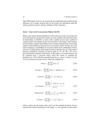
Morphological operations use a structuring element to calculate new pixels,
which plays the role of a neighborhood or convolution kernel in other image
processing operations (as shown in filter mask operations). Figure 2.11 shows two
typical examples of structuring elements. The shape of the structuring element
could be rectangular, square, diamond, octagon, disk, etc. The connectivity defines
whether four or all eight surrounding pixels are used to calculate the new center
pixel value (in the case of a [33] structuring element) (Klinger 2003).
2.4.5.1 Erosion and Dilation
These two operators are fundamental for almost all morphological operations
(Gonzales and Woods 2008). Opening and closing are also duals of each other
with respect to set complementation and reflection. Thus, Erosion is an operator
that basically removes objects smaller than the structuring element and removes
perimeter pixels from the border of larger image objects (sets the pixel value to 0).
If I is an image and M is the structuring element (mask), the erosion (operator ) is
defined as:
erosion I
ð Þ ¼ I M ¼ a2MIa ð2:39Þ
where Ia indicates a basic shift operation in the direction of element a of M and Ia
would indicate the reverse shift operation.
Contrarily, a dilation operation enlarges a region. A dilation adds pixels to the
perimeter of each image object (sets their values to 1), filling in holes and broken
0 1 0
1 1
0 1 0
1 1 1
1 1
1 1 1
a b
Origin of the [3×3]
structuring element
Fig. 2.11 Examples of
square structuring elements
(a) connectivity 4;
(b) connectivity 8
2 Basics of Image Analysis 35](https://image.slidesharecdn.com/2015-220313111348/85/2015-basicsof-imageanalysischapter2-1-28-320.jpg)


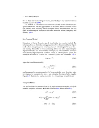
![the attenuation coefficient histogram and the nature of X-ray tomography (where
processing and analysis are based on voxels instead of pixels). Moreover, the
resulting binary image of apple tissue using global thresholds of 60 is noisy
(Fig. 2.13b), and the average porosity is highly dependent on the selected thres-
hold value. Figure 2.13e plots the distribution of the transmitted X-ray intensities
(solid line, right axis) measured for the reconstructed tomography images of apple
tissue, and it also shows the typical dependence of the porosity (open circles,
left axis) of the resulting segmented image when a simple global threshold
is chosen.
Grayscale intensities
0 25 50 75 100 125 150 175 200 225 250
0
2000
4000
6000
8000
10000
12000
14000
16000
Number
of
pixels
Stage 1
Stage 5
banana
background
60
Segmented RGB image
Binary image
Threshold = 60
Ripening stage 5
Gray scale image
Ripening stage 1
a
b
Fig. 2.12 Image segmentation process for bananas using a simple global thresholding:
(a) pre-processing of a color image of bananas in ripening stages 1 and 5, including previous
grayscale transformation and image smoothing using a Laplacian-of-Gaussian filter (LOG filter)
[3 3] for easing the edge detection, binarization, and segmentation; (b) histogram of the
grayscale images for both bananas showing the chosen threshold value of 60
38 F. Mendoza and R. Lu](https://image.slidesharecdn.com/2015-220313111348/85/2015-basicsof-imageanalysischapter2-1-31-320.jpg)


![spite of the complexity and high variability in color and texture appearance, the
modeling of ham slice images with DFD allowed the capture of differentiating
textural features between the four commercial ham types. Independent DFD
features entailed better discrimination than that using the average of four directions.
However, the DFD features revealed a high sensitivity to color channel, orientation
and image resolution for the fractal analysis. The classification accuracy using six
DFD features was 93.9 % for the training data and 82.2 % for the testing data.
Fourier Fractal Texture (FFT)
In the calculation of FFT, the 2D Fourier transform of the grayscale image is first
calculated and the 2D power spectrum is then derived. The 2D power spectrum is
reduced to a 1D radial power spectrum (direction-independent mean spectrum, i.e., the
average of all possible directional power spectra) by averaging values over increas-
ingly larger annuli for each of the radial increments. The power spectrum, P( f ),
varying with frequency f, is calculated as follows (Dougherty and Henebry 2001):
P f
ð Þ ¼ k f 12H
ð Þ
ð2:70Þ
where k is a constant and H is the Hausdorff-Besicovitch dimension. When the log
[P( f )] is plotted against log[f], a straight line can be fitted. According to the Fourier
slice theorem, the 1D Fourier transform of a parallel projection of an image along a
line with the direction h is identical to the value along the same line in the 2D
Fourier transform of the image. This means that the line through the spectrum gives
the spectral information obtained from a projection with the same orientation in the
spatial domain. FFT dimensions, Df, are calculated as a function of orientation
based on this theorem, with 24 being the frequently number of directions that the
frequency space is uniformly divided. The data of magnitude vs. frequency are
plotted in log-log scale and its slope is determined using linear least-squares
regression. Thus, Hausdorff-Besicovitch dimension H is computed from the slope
c of the straight line, c ¼ (12H). The Df dimension of the grayscale image is
related to the slope c of the log–log plot by the equation below, with H ¼ Df3,
2 Df 3 and 3 c 1 (Geraets and Van der Stelt 2000):
D f ¼
7
2
þ
c
2
ð2:71Þ
For analysis the slope and intercept for all directions can be computed from each
image and used for further image characterization and classification. This algorithm
was proposed by Russ (2005) and was modified by Valous et al. (2009b) for hams
processing.
2 Basics of Image Analysis 49](https://image.slidesharecdn.com/2015-220313111348/85/2015-basicsof-imageanalysischapter2-1-42-320.jpg)