Downloaded 28 times


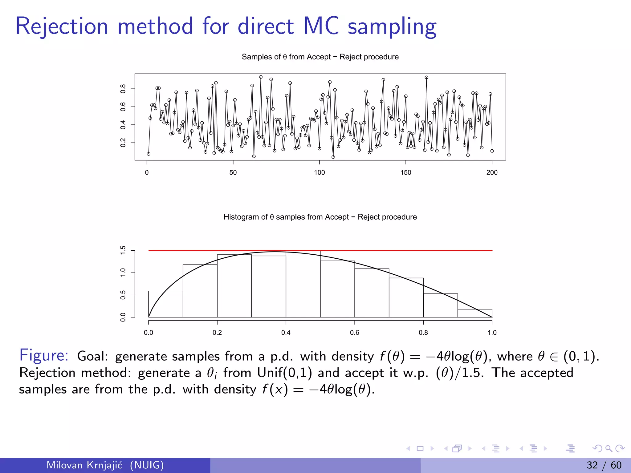
![Monte Carlo (MC) sampling
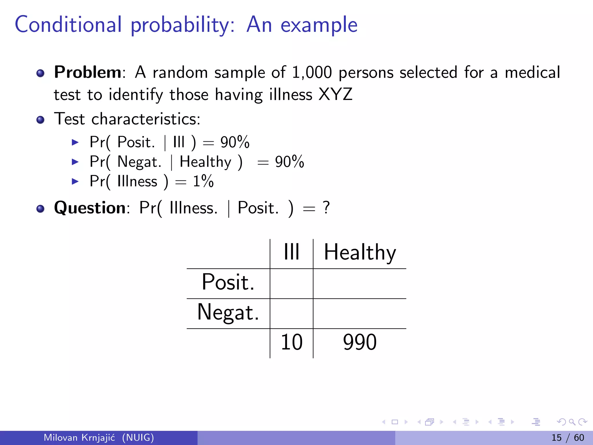
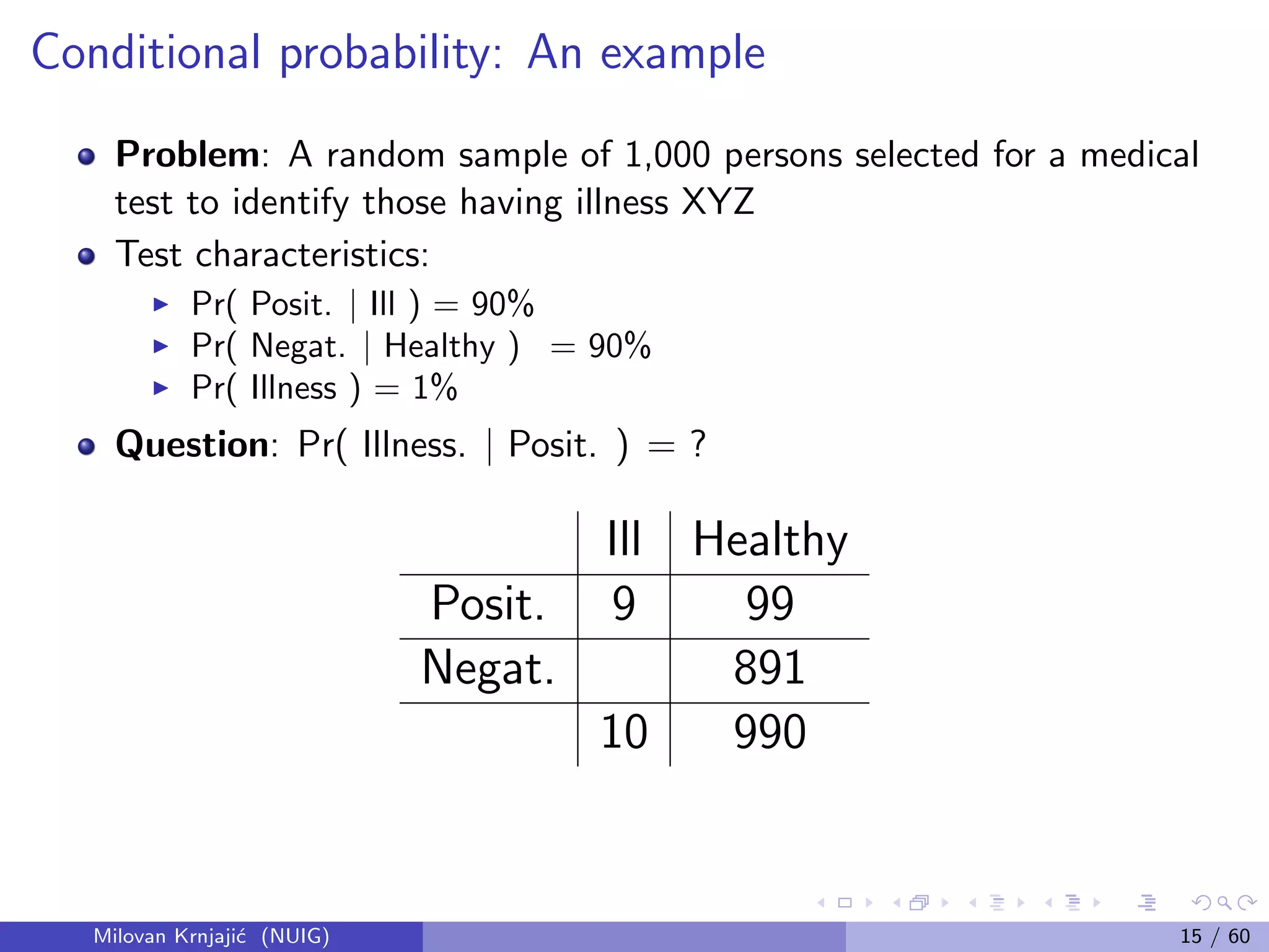
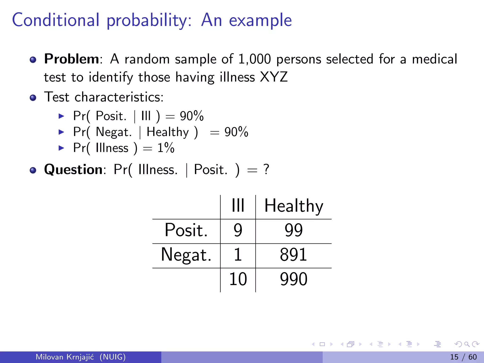
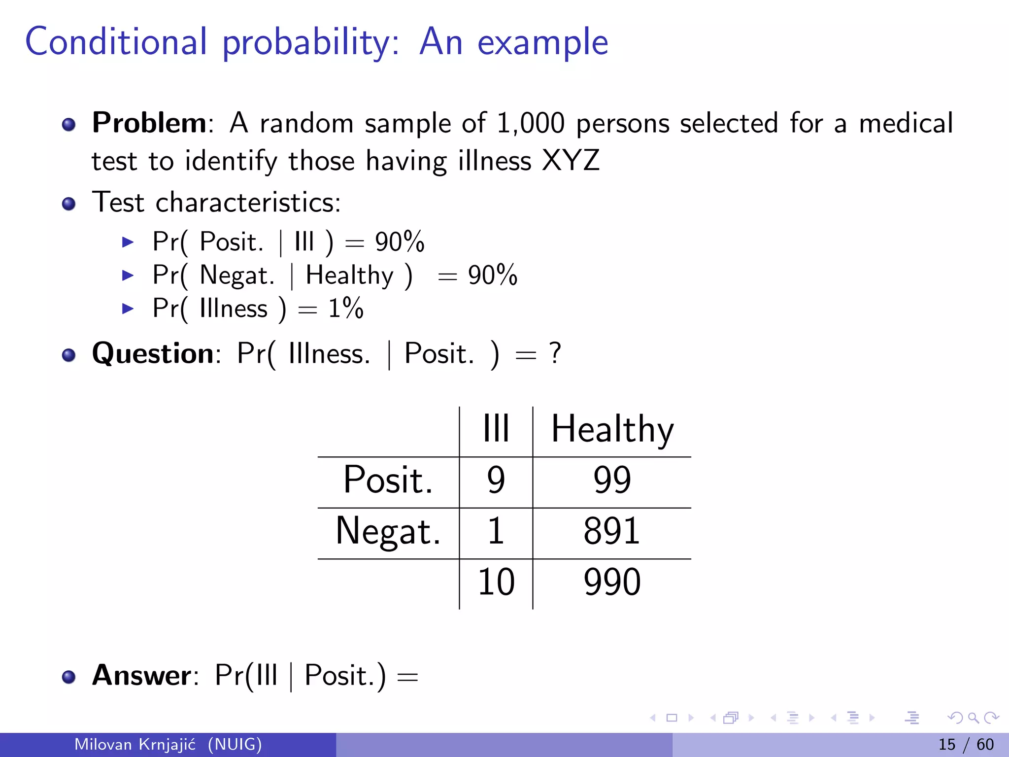
In practice, p(θ | y) = p(θ) × L(θ | y), complex and dim(θ) large
Problem: no closed form for integrals; no numerical integration;
A solution: Can learn anything about a probability
distribution from a large sample.
If xi ∼ p(x) then 1
n
n
i=1 g(xi ) → E[g(X)] = X g(x)p(x)dx
Instead of maths – simulation: generate independent samples from
the joint posterior distribution
Milovan Krnjaji´c (NUIG) 31 / 60](https://image.slidesharecdn.com/2013-140724081706-phpapp02/75/2013-03-26-Bayesian-Methods-for-Modern-Statistical-Analysis-41-2048.jpg)

![Bayesian decision theory
Bayesian decision theory: rational and coherent decisions are made
based on maximization of the expected utility function.
Let A be a set of possible actions, U(a, θ) the utility function, action
a, where the unknown info is θ;
The optimal actions a∗ maximizes the expectation of U:
E(θ|y) [U(a, θ)]
This approach has been succesfully used in many areas, such as
business management, econometrics, engineering, health care,
medicine, etc.
Milovan Krnjaji´c (NUIG) 37 / 60](https://image.slidesharecdn.com/2013-140724081706-phpapp02/75/2013-03-26-Bayesian-Methods-for-Modern-Statistical-Analysis-47-2048.jpg)

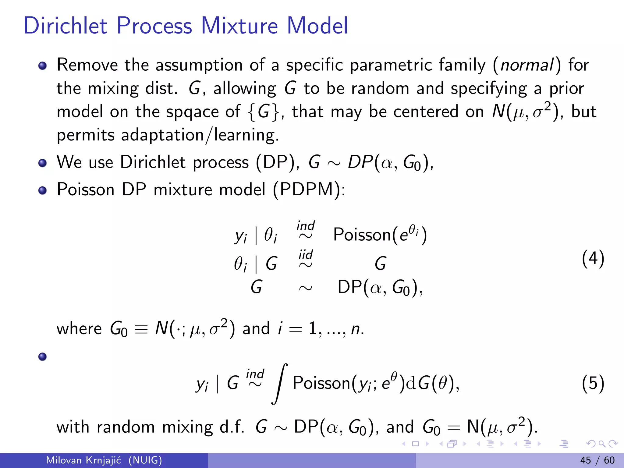
![Modelling of Count Data
Example: Count data — Bayesian parametric Poisson based model vs.
Bayesian nonparametric (BNP) with a Dirichlet process prior.
Fixed-effects Poisson model, (for i = 1, . . . , n),
(yi |θ)
ind
∼ Poisson[exp(θ)]
(θ|µ, σ2
)
iid
∼ N(µ, σ2
)
(µ, σ2
) ∼ p(µ, σ2
).
(2)
This uses a Lognormal prior for λ = eθ
rather than conjugate Gamma choice;
the two families are similar, and the Lognormal generalizes more readily.
Data often exhibit heterogeneity resulting in (extra-Poisson variability),
variance-to-mean ratio, VTMR > 1
Milovan Krnjaji´c (NUIG) 43 / 60](https://image.slidesharecdn.com/2013-140724081706-phpapp02/75/2013-03-26-Bayesian-Methods-for-Modern-Statistical-Analysis-53-2048.jpg)
![Parametric Random-Effects Poisson (PREP) Model
Random-effects Poisson model (PREP):
(yi |θi )
ind
∼ Poisson[exp(θi )]
(θi |G)
iid
∼ G
G ≡ N(µ, σ2)
(µ, σ2) ∼ p(µ, σ2),
(3)
assuming a parametric CDF G (the Gaussian) for the latent variables
or random effects θi .
Distribution, G, in the population to which it’s appropriate to
generalize may be multimodal or skewed, which a single Gaussian
can’t capture; if so, this PREP model can fail to be valid.
Milovan Krnjaji´c (NUIG) 44 / 60](https://image.slidesharecdn.com/2013-140724081706-phpapp02/75/2013-03-26-Bayesian-Methods-for-Modern-Statistical-Analysis-54-2048.jpg)


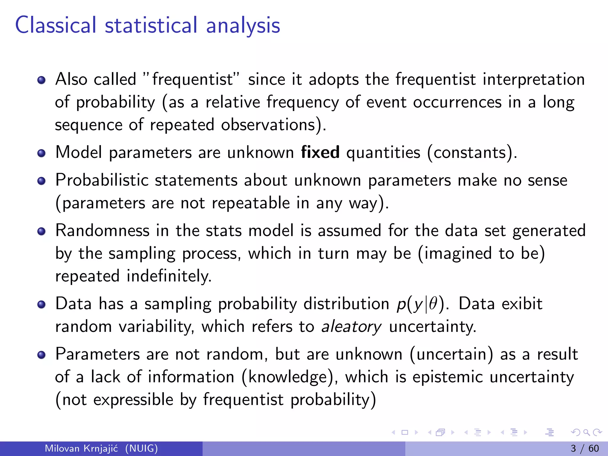
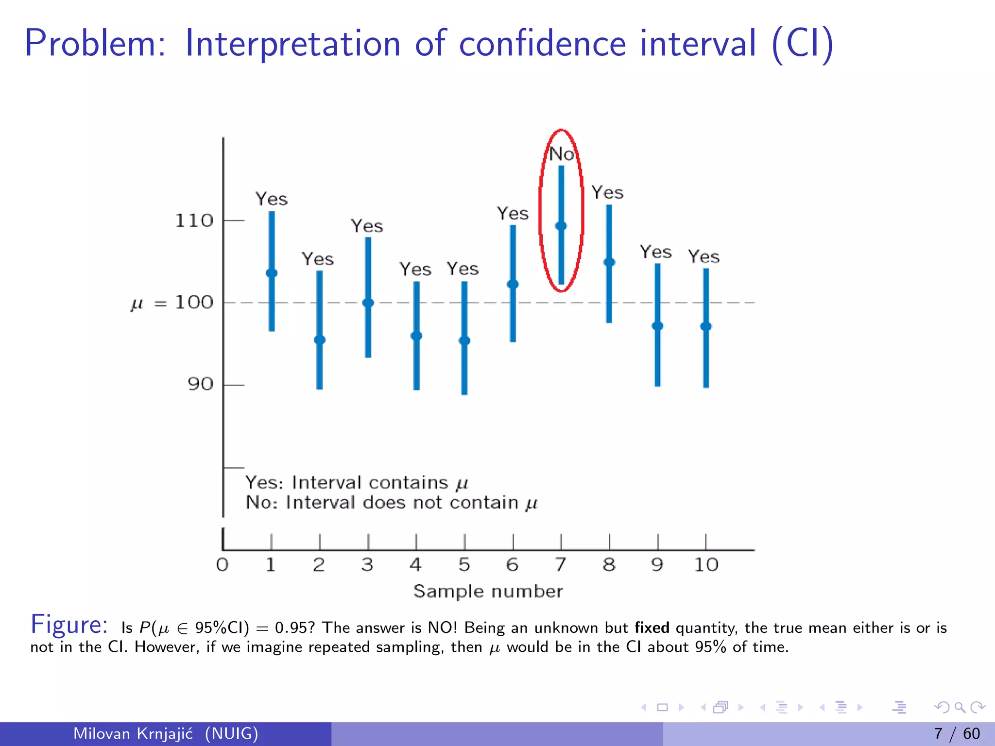
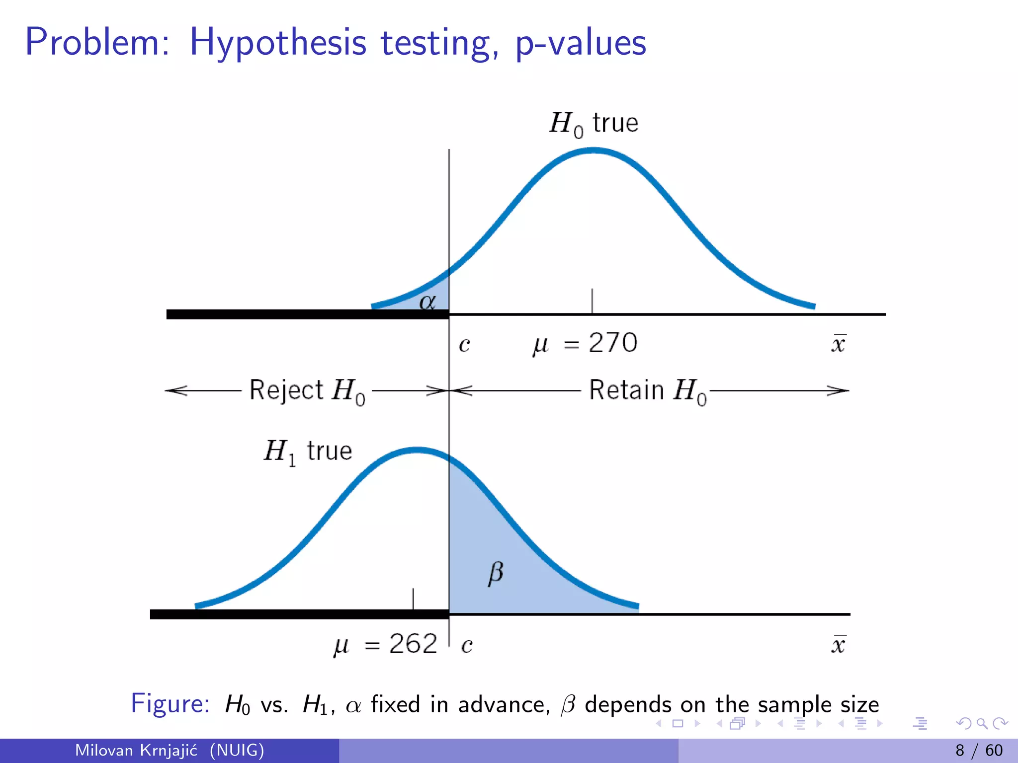
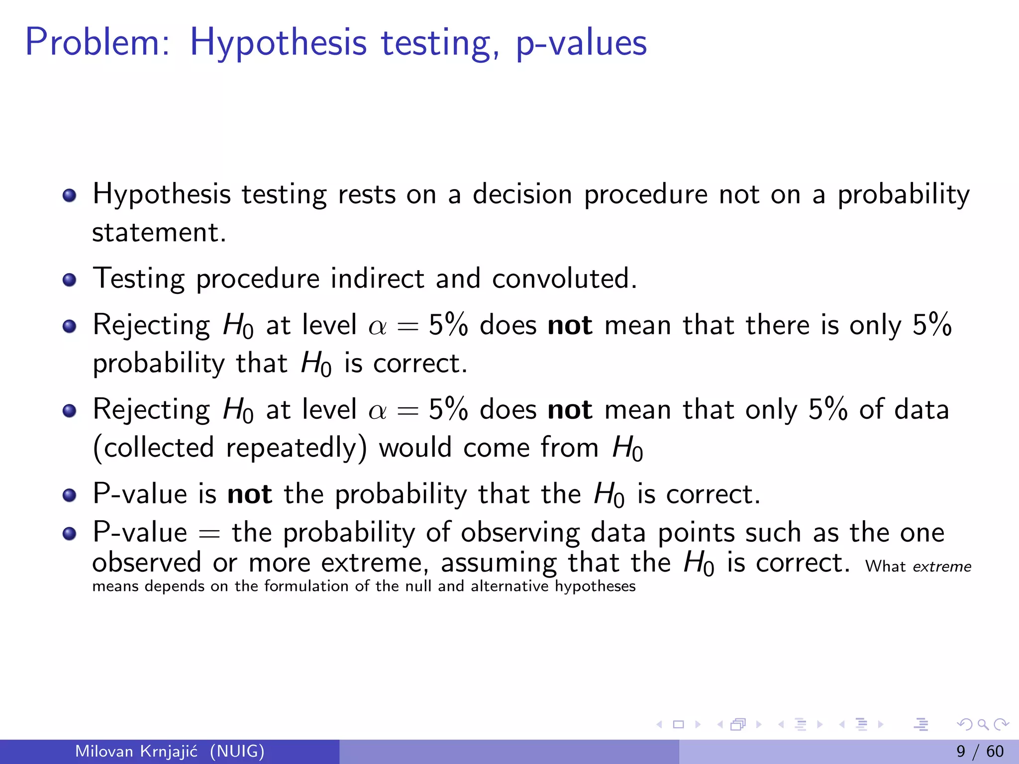
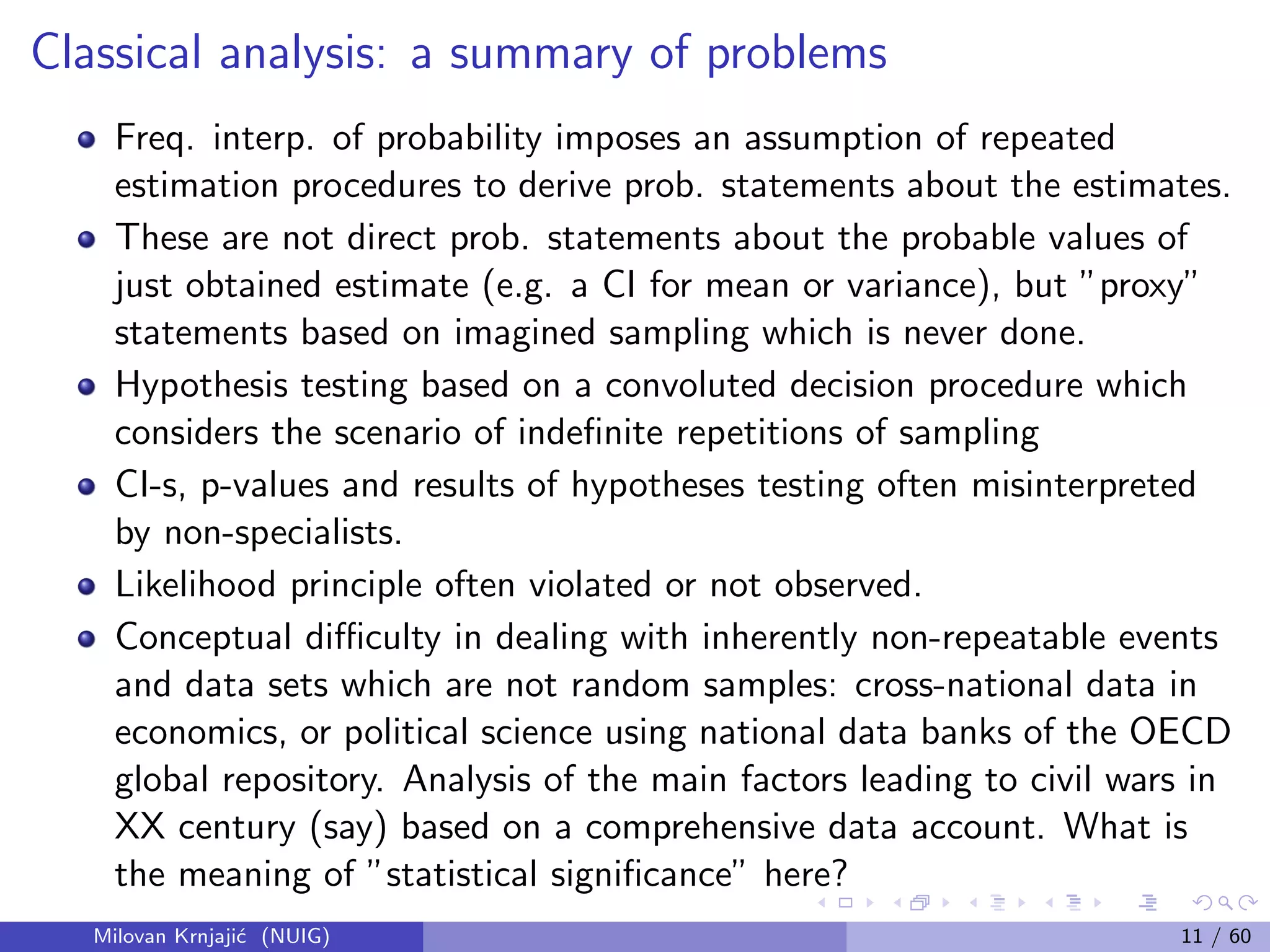
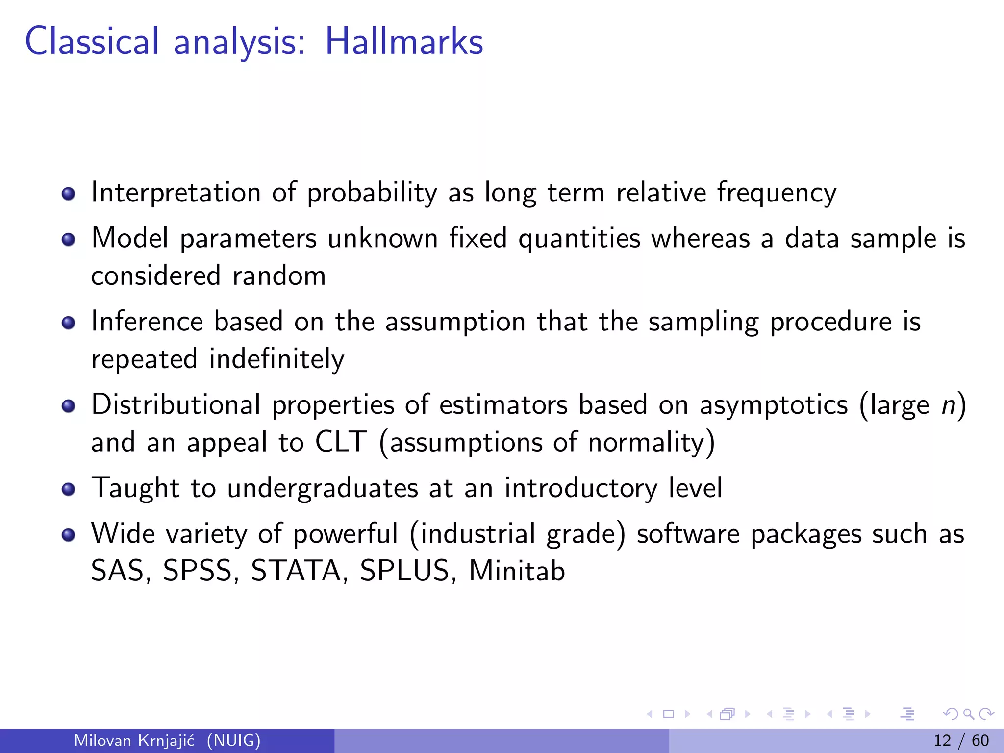
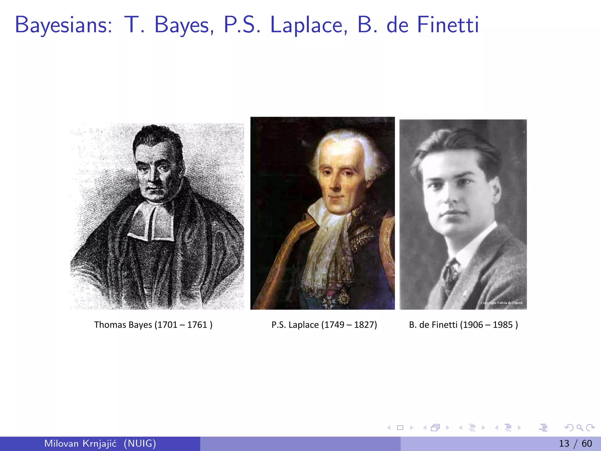
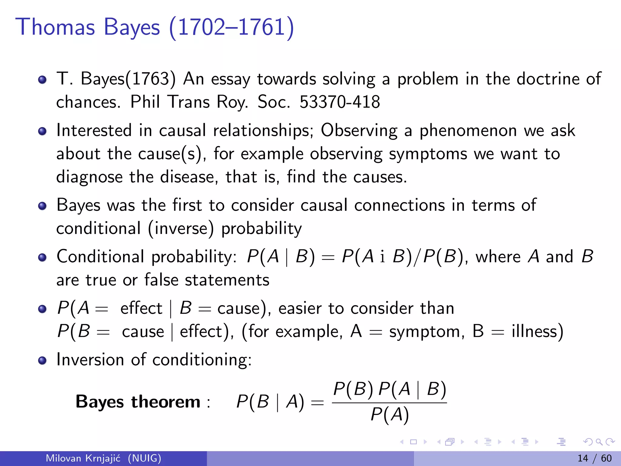
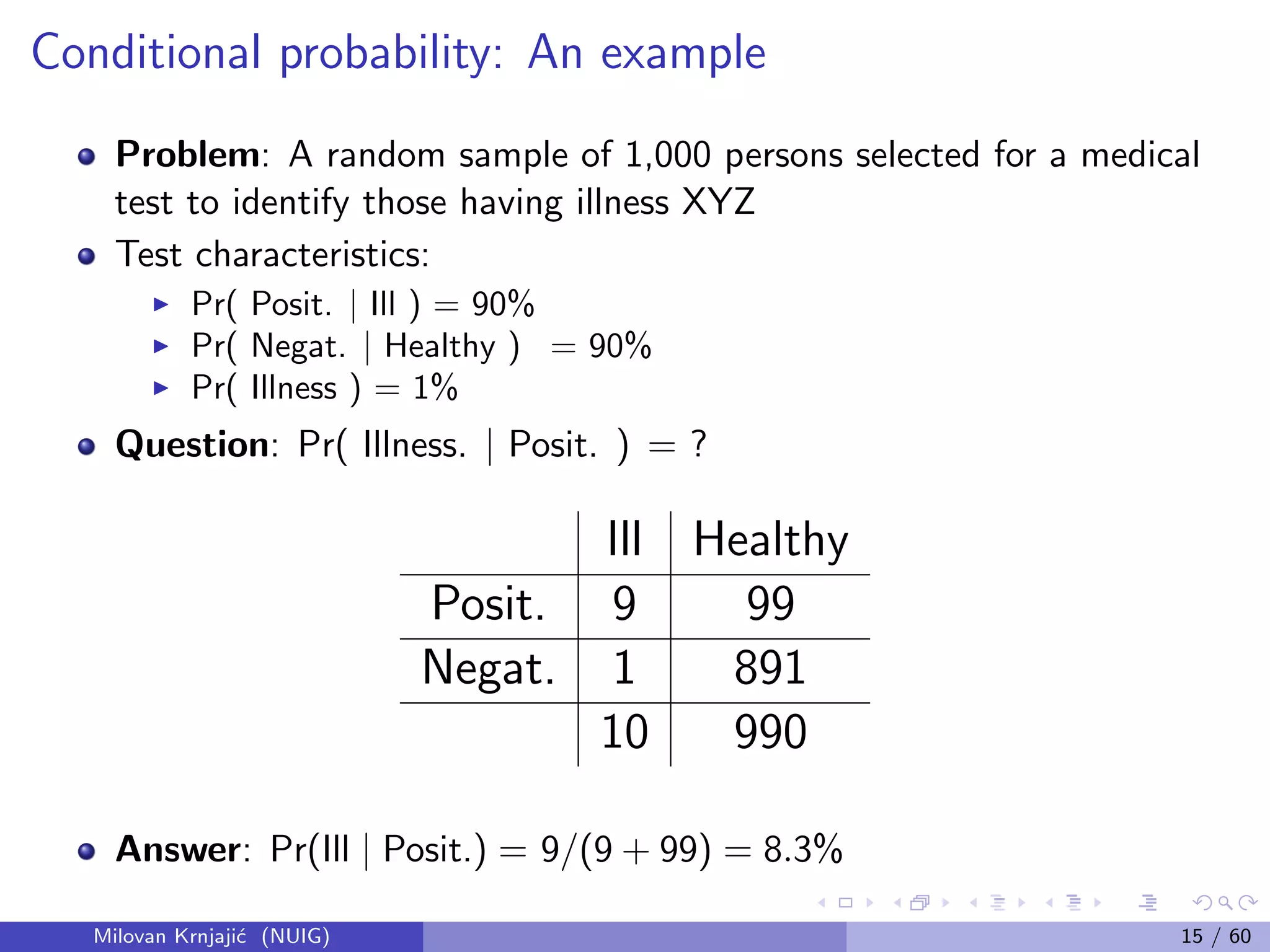
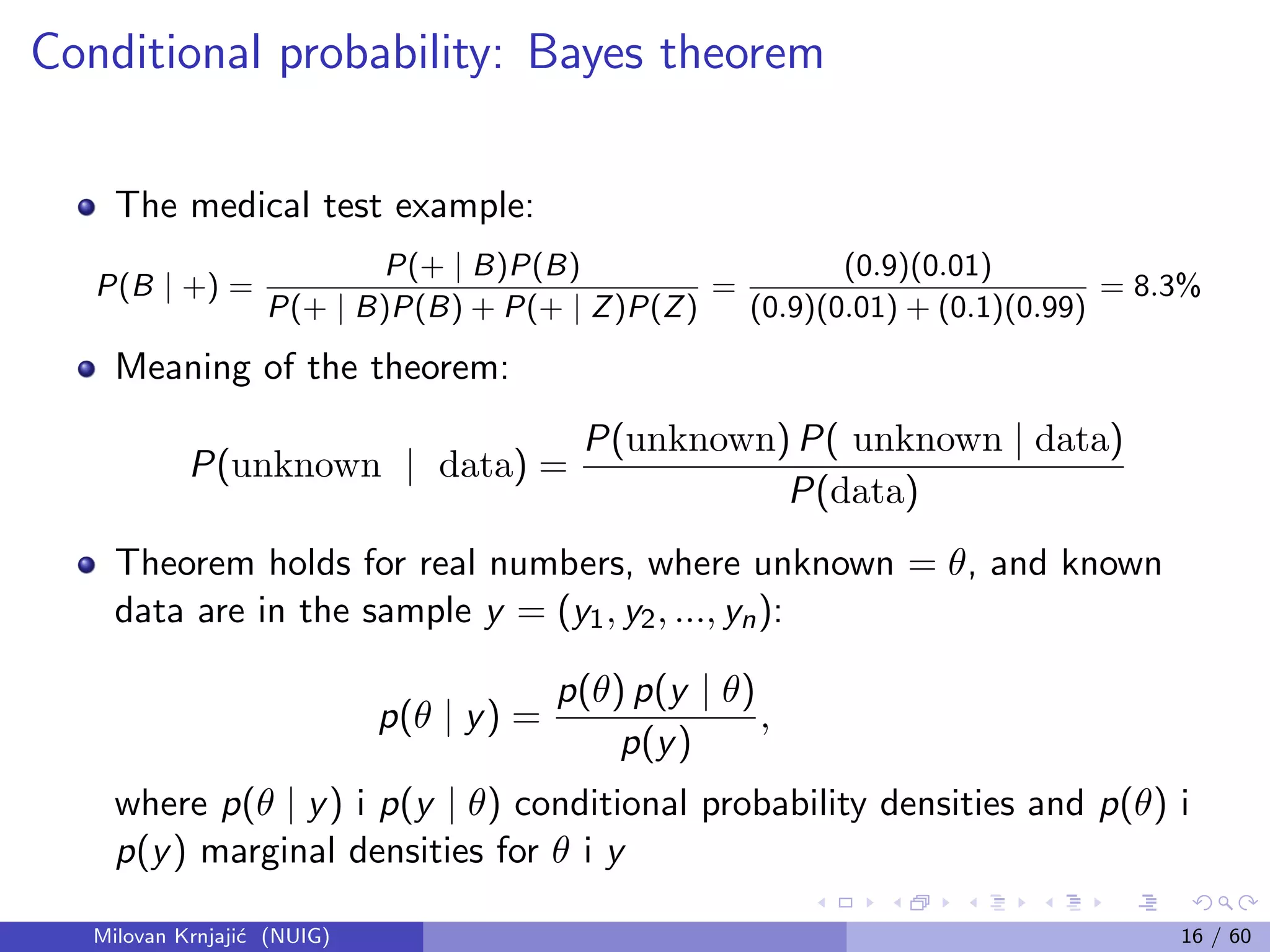
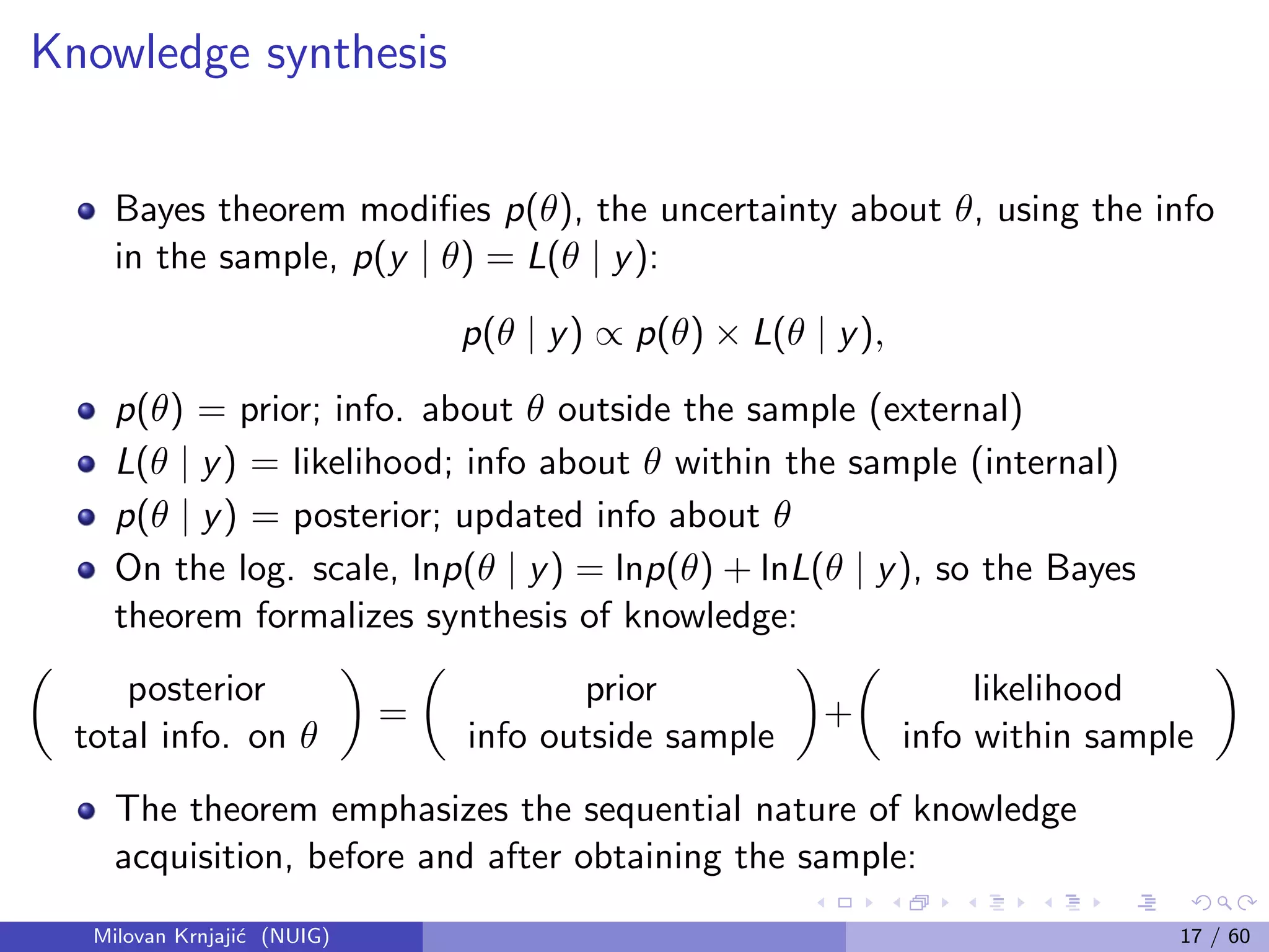
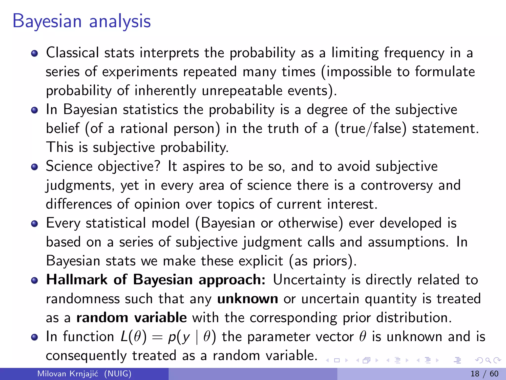
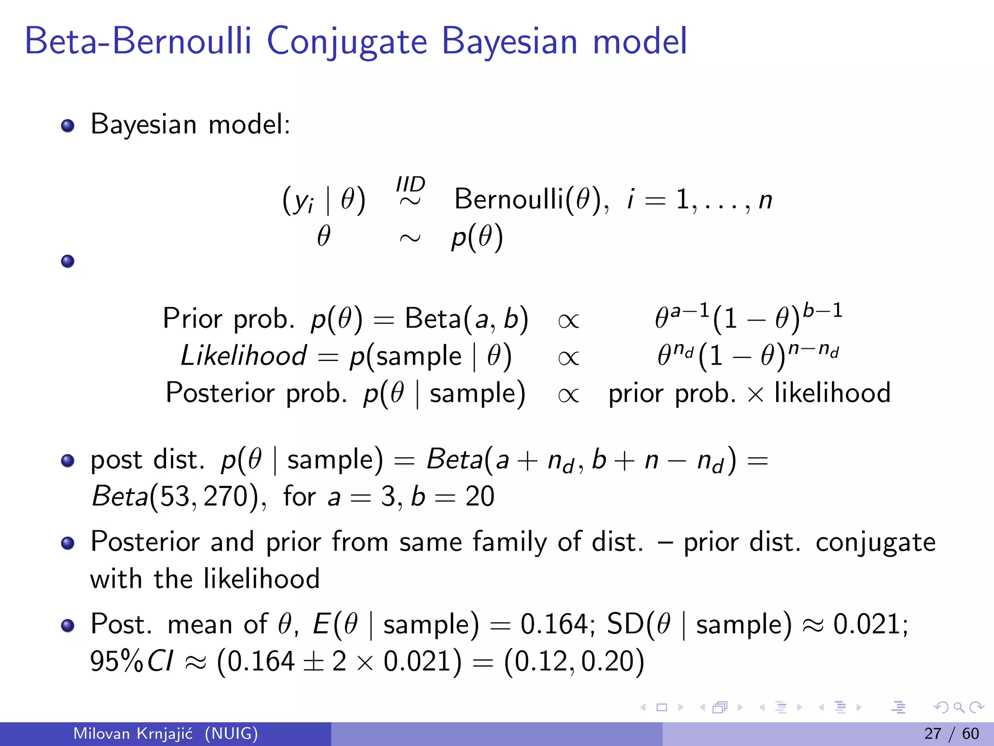
This document provides an overview of Bayesian statistical analysis compared to classical frequentist approaches. It discusses some key problems with classical methods like misinterpretation of confidence intervals and p-values. Bayesian analysis uses Bayes' theorem to update the prior probability of parameters based on observed data, synthesizing external prior information with internal sample information. This provides a unified framework for statistical inference that does not require imagining hypothetical repeated samples. The document also introduces some important figures in the development of Bayesian statistics like Thomas Bayes, Pierre-Simon Laplace, and Bruno de Finetti.


![[DSC Europe 25] Andy Cotgreave - Nothing is new in analytics.pptx](https://cdn.slidesharecdn.com/ss_thumbnails/mba4vzcurvoh5lfrd5zw-6-251205194645-341bbbbe-thumbnail.jpg?width=640&height=640&fit=bounds)


![[DSC Europe 25] Max Talanov - Non digital NNs.pptx](https://cdn.slidesharecdn.com/ss_thumbnails/wif8tr3gtua74qvtopke-non-digital-nns-251205090438-26b0eea6-thumbnail.jpg?width=640&height=640&fit=bounds)


![[DSC Europe 25] Jim Sterne - Adopting Generative AI Capabilities Into the Ent...](https://cdn.slidesharecdn.com/ss_thumbnails/sxhpofuorcagxsaulkmt-3-251204082258-7e66bc48-thumbnail.jpg?width=640&height=640&fit=bounds)


![[DSC Europe 25] Boris Perkovic - Lost in performance.pptx](https://cdn.slidesharecdn.com/ss_thumbnails/uq5hrp7vsuahqkxzifux-1-251204082258-fd2ee09d-thumbnail.jpg?width=640&height=640&fit=bounds)

![[DSC Europe 25] Bogdan Daniel Maruneac - AI - It starts with you.pptx](https://cdn.slidesharecdn.com/ss_thumbnails/odov3snhrcqs9hx5ny2n-4-251205085715-f1daacfe-thumbnail.jpg?width=640&height=640&fit=bounds)
![[DSC Europe 25] Dusan Jovicic - AI Story: From on-prem to cloud and back agai...](https://cdn.slidesharecdn.com/ss_thumbnails/8kp49m6uq22ifnbwhfnk-2-251205085715-964d11a6-thumbnail.jpg?width=640&height=640&fit=bounds)
![[DSC Europe 25] Nikola Rajovic - Hardware Technologies Under the Hood: RISC-V...](https://cdn.slidesharecdn.com/ss_thumbnails/o2gptrmtoyqndgoshwgq-dsc2025-tenstorrent-rajovic-251205090438-814685f5-thumbnail.jpg?width=640&height=640&fit=bounds)