Chap6-ClassificationBasic_data_mining.pdf

1
Chapter 6. Classification: Basic Concepts
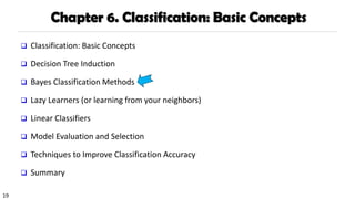
❑ Classification: Basic Concepts
❑ Decision Tree Induction
❑ Bayes Classification Methods
❑ Lazy Learners (or learning from your neighbors)
❑ Linear Classifiers
❑ Model Evaluation and Selection
❑ Techniques to Improve Classification Accuracy
❑ Summary

2
Supervised vs. Unsupervised Learning (1)
❑ Supervised learning (classification)
❑ Supervision: The training data such as observations or measurements are
accompanied by labels indicating the classes which they belong to
❑ New data is classified based on the models built from the training set
Training Data with class label:
Model
Learning
Positive
Negative
Training
Instances
Test
Instances
Prediction
Model
Outlook Temp Humidity Windy Play Golf
Rainy Hot High False No
Rainy Hot High True No
Overcast Hot High False Yes
Sunny Mild High False Yes
Sunny Cool Normal False Yes
Sunny Cool Normal True No
Overcast Cool Normal True Yes
Rainy Mild High False No

3
Supervised vs. Unsupervised Learning (2)
❑ Unsupervised learning (clustering)
❑ The class labels of training data are unknown
❑ Given a set of observations or measurements, establish the possible existence
of classes or clusters in the data

4
❑ Classification
❑ Predict categorical class labels (discrete or nominal)
❑ Construct a model based on the training set and the class labels (the values in a
classifying attribute) and use it in classifying new data
❑ Numeric prediction
❑ Model continuous-valued functions (i.e., predict unknown or missing values)
Prediction Problems: Classification vs. Numeric Prediction

5
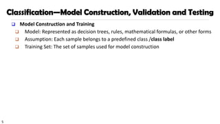
Classification—Model Construction, Validation and Testing
❑ Model Construction and Training
❑ Model: Represented as decision trees, rules, mathematical formulas, or other forms
❑ Assumption: Each sample belongs to a predefined class /class label
❑ Training Set: The set of samples used for model construction

6
Classification—Model Construction, Validation and Testing
❑ Model Validation and Testing:
❑ Test: Estimate accuracy of the model
❑ The known label of test sample VS. the classified result from the model
❑ Accuracy: % of test set samples that are correctly classified by the model
❑ Test set is independent of training set
❑ Validation: If the test set is used to select or refine models, it is called validation (or
development) (test) set
❑ Model Deployment: If the accuracy is acceptable, use the model to classify new data

7
❑ Summary

8
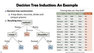
Decision Tree Induction: An Example
outlook?
windy? Humidity?
Sunny Rainy
Yes No No
Overcast
Yes
High
Normal
True
False
❑ Decision tree construction:
❑ A top-down, recursive, divide-and-
conquer process
❑ Resulting tree:
Training data set: Play Golf?
Yes
Outlook Temp Humidity Windy Play Golf
Rainy Cool Normal False Yes
Sunny Mild Normal False Yes
Rainy Mild Normal True Yes
Overcast Mild High True Yes
Overcast Hot Normal False Yes
Sunny Mild High True No
https://www.saedsayad.com/decision_tree.htm

9
Decision Tree Induction: Algorithm
❑ Basic algorithm
❑ Tree is constructed in a top-down, recursive, divide-and-conquer manner
❑ At start, all the training examples are at the root
❑ Examples are partitioned recursively based on selected attributes
❑ On each node, attributes are selected based on the training examples on that
node, and a heuristic or statistical measure (e.g., information gain, Gini index)

10
Decision Tree Induction: Algorithm
❑ Conditions for stopping partitioning
❑ All samples for a given node belong to the same class
❑ There are no remaining attributes for further partitioning
❑ There are no samples left
❑ Prediction
❑ Majority voting is employed for classifying the leaf

11
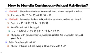
How to Handle Continuous-Valued Attributes?
❑ Method 1: Discretize continuous values and treat them as categorical values
❑ E.g., age: < 20, 20..30, 30..40, 40..50, > 50
❑ Method 2: Determine the best split point for continuous-valued attribute A
❑ Sort:, e.g. 15, 18, 21, 22, 24, 25, 29, 31, …
❑ Possible split point: (ai+ai+1)/2
❑ e.g., (15+18)/2 = 16.5, 19.5, 21.5, 23, 24.5, 27, 30, …
❑ The point with the maximum information gain for A is selected as the split-
point for A
❑ Split: Based on split point P
❑ The set of tuples in D satisfying A ≤ P vs. those with A > P

12
Pro’s and Con’s
❑ Pro’s
❑ Easy to explain (even for non-expert)
❑ Easy to implement (many software)
❑ Efficient
❑ Can tolerant missing data
❑ White box
❑ No need to normalize data
❑ Non-parametric: No assumption on data distribution, no assumption on
attribute independency
❑ Can work on various attribute types

13
Con’s
❑ Con’s
❑ Unstable. Sensitive to noise
❑ Accuracy may be not good enough (depending on your data)
❑ The optimal splitting is NP. Greedy algorithms are used
❑ Overfitting

14
Splitting Measures: Information Gain
❑ Entropy (Information Theory)
❑ A measure of uncertainty associated with a random number
❑ Calculation: For a discrete random variable Y taking m distinct values {y1, y2, …, ym}
❑ Interpretation
❑ Higher entropy → higher uncertainty
❑ Lower entropy → lower uncertainty
❑ Conditional entropy
m = 2

15
Information Gain: An Attribute Selection Measure
❑ Select the attribute with the highest information gain (used in typical
decision tree induction algorithm: ID3/C4.5)
❑ Let pi be the probability that an arbitrary tuple in D belongs to class Ci,
estimated by |Ci, D|/|D|
❑ Expected information (entropy) needed to classify a tuple in D:
❑ Information needed (after using A to split D into v partitions) to classify D:
❑ Information gained by branching on attribute A
)
(
log
)
( 2
1
i
m
i
i p
p
D
Info 
=
−
=
)
(
|
|
|
|
)
(
1
j
v
j
j
A D
Info
D
D
D
Info 
= 
=
(D)
Info
Info(D)
Gain(A) A
−
=

16
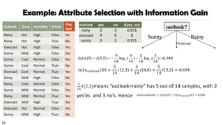
Example: Attribute Selection with Information Gain
5
14
𝐼(2,3)means “outlook=rainy” has 5 out of 14 samples, with 2
yes’es and 3 no’s. Hence 𝐺𝑎𝑖𝑛(𝑜𝑢𝑡𝑙𝑜𝑜𝑘) = 𝐼𝑛𝑓𝑜(𝐷) − 𝐼𝑛𝑓𝑜𝑜𝑢𝑡𝑙𝑜𝑜𝑘(𝐷) = 0.246
outlook?
Sunny Rainy
Overcast
940
.
0
)
14
5
(
log
14
5
)
14
9
(
log
14
9
)
5
,
9
(
)
( 2
2 =
−
−
=
= I
D
Info
outlook yes no I(yes, no)
rainy 2 3 0.971
overcast 4 0 0
sunny 3 2 0.971
𝐼𝑛𝑓𝑜𝑜𝑢𝑡𝑙𝑜𝑜𝑘 𝐷 =
5
14
𝐼 2,3 +
4
14
𝐼 4,0 +
5
14
𝐼 3,2 = 0.694
Outlook Temp Humidity Windy
Play
Golf

17
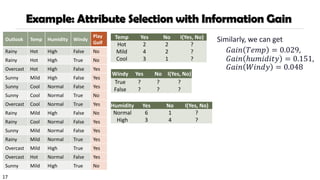
Example: Attribute Selection with Information Gain
Similarly, we can get
𝐺𝑎𝑖𝑛 𝑇𝑒𝑚𝑝 = 0.029,
𝐺𝑎𝑖𝑛 ℎ𝑢𝑚𝑖𝑑𝑖𝑡𝑦 = 0.151,
𝐺𝑎𝑖𝑛 𝑊𝑖𝑛𝑑𝑦 = 0.048
Temp Yes No I(Yes, No)
Hot 2 2 ?
Mild 4 2 ?
Cool 3 1 ?
Humidity Yes No I(Yes, No)
Normal 6 1 ?
High 3 4 ?
Windy Yes No I(Yes, No)
True ? ? ?
False ? ? ?
Outlook Temp Humidity Windy
Play
Golf

18
Gain Ratio: A Refined Measure for Attribute Selection
❑ Information gain measure is biased towards attributes with a large number of
values (e.g. ID)
❑ Gain ratio: Overcomes the problem (as a normalization to information gain)
❑ GainRatio(A) = Gain(A)/SplitInfo(A)
❑ The attribute with the maximum gain ratio is selected as the splitting attribute
❑ Gain ratio is used in a popular algorithm C4.5 (a successor of ID3) by R. Quinlan
❑ Example
❑ SplitInfotemp D = −
4
14
log2
4
14
−
6
14
log2
6
14
−
4
14
log2
4
14
= 1.557
❑ GainRatio(temp) = 0.029/1.557 = 0.019
)
|
|
|
|
(
log
|
|
|
|
)
( 2
1 D
D
D
D
D
SplitInfo
j
v
j
j
A 
−
= 
=

19
❑ Summary

20
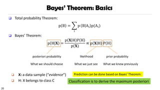
Bayes’ Theorem: Basics
❑ Total probability Theorem:
p B = ෍
i
p B Ai p(Ai)
❑ Bayes’ Theorem:
p H|𝐗 =
p 𝐗 H P H
p(𝐗)
∝ p 𝐗 H P H
❑ X: a data sample (“evidence”)
❑ H: X belongs to class C
posteriori probability prior probability
likelihood
What we should choose What we knew previously
What we just see
Prediction can be done based on Bayes’ Theorem:
Classification is to derive the maximum posteriori

21
Bayes’ Theorem Example: Picnic Day
❑ The morning is cloudy 
❑ What is the chance of rain?
❑ 50% of all rainy days start off cloudy.
❑ Cloudy mornings are common (40% of days start cloudy)
❑ This is usually a dry month (only 3 of 30 days tend to be rainy)
❑ The chance of rain is probably not as high as expected ☺
❑ Bayes’ Theorem allows us to tell back and forth between posterior and likelihood
(e.g., P(Rain | Cloud) and P(Cloud | Rain)), tests the reality, which is the most
important trick in Bayesian Inference
P(Cloud) = 40%
P(Rain) = 10%
P(Cloud | Rain) = 50%
P(Rain | Cloud) = P(Rain) P(Cloud | Rain) / P(Cloud) = 10% * 50% / 40% = 12.5%
P(Rain | Cloud) = ?

22
Naïve Bayes Classifier: Making a Naïve Bayes Assumption
❑ Based on the Bayes’ Theorem, we can derive a Bayes Classifier to compute the
posterior probability of classifying an object X to a class C
❑ P (C|X) ∝ P(X|C)P(C) = P(x1|C)P(x2|x1,C)...P(xn|x1,...,C)P(C)
❑ A naïve bayes assumption to simplify the complex dependencies: features are
conditionally independent, given the class label!
❑ P (C|X) ∝ P(X|C)P(C) ≈ P(x1|C)P(x2|C)...P(xn|C)P(C)
❑ Super efficient: each feature only conditions on the class (boils down to sample
counting)
❑ Achieves surprisingly comparable performance

23
Naïve Bayes Classifier: Categorical vs. Continuous Valued Features
❑ If feature xk is categorical, p(xk = vk|Ci) is the # of tuples in Ci with xk = vk,
divided by |Ci, D| (# of tuples of Ci in D)
❑ If feature xk is continuous-valued, p(xk = vk|Ci) is usually computed based on
Gaussian distribution with a mean μ and standard deviation σ
p xk = vk Ci = 𝑁 xk μCi
, σCi
=
1
2πσCi
𝑒
−
𝑥−𝜇𝐶𝑖
2
2𝜎2
p X|𝐶𝑖 = ςk p xk Ci) = p x1 Ci) ∙ p x2 Ci) ∙∙∙∙∙ p xn Ci)

24
Naïve Bayes Classifier Example 1: Training Dataset
Class:
play golf= ‘yes’
play golf = ‘no’

25
Naïve Bayes Classifier Example P(Yes | Sunny)

26
Naïve Bayes Classifier Example: P(No | Sunny)

27
Naïve Bayes Classifier Example: Likelihood Tables

28
Naïve Bayes Classifier Example: Likelihood Tables
P(x) = P( x | yes ) * P (yes) + P( x | no ) * P (no)
/ P(x)
/ P(x)
______________________
P(x)
______________________
P(x)

29
Avoiding the Zero-Probability Problem
❑ Naïve Bayesian prediction requires each conditional probability be non-zero
❑ Otherwise, the predicted probability will be zero
❑ Example. Suppose a dataset with 1,000 tuples:
income = low (0), income= medium (990), and income = high (10)
❑ Use Laplacian correction (or Laplacian estimator)
❑ Adding 1 (or a small integer) to each case
Prob(income = low) = 1/(1000 + 3)
Prob(income = medium) = (990 + 1)/(1000 + 3)
Prob(income = high) = (10 + 1)/(1000 + 3)
❑ The “corrected” probability estimates are close to their “uncorrected”
counterparts
p X|𝐶𝑖 = ς𝑘 𝑝 𝑥𝑘 𝐶𝑖) = 𝑝 𝑥1 𝐶𝑖) ∙ 𝑝 𝑥2 𝐶𝑖) ∙∙∙∙∙ 𝑝 𝑥𝑛 𝐶𝑖)

30
Naïve Bayes Classifier: Strength vs. Weakness
❑ Strength
❑ Performance: A naïve Bayesian classifier, has comparable performance with
decision tree and selected neural network classifiers
❑ Incremental: Each training example can incrementally increase/decrease the
probability that a hypothesis is correct—prior knowledge can be combined with
observed data

31
Naïve Bayes Classifier: Strength vs. Weakness
❑ Weakness
❑ Assumption: attributes conditional independence, therefore loss of accuracy
❑ E.g., Patient’s Profile: (age, family history),
❑ Patient’s Symptoms: (fever, cough),
❑ Patient’s Disease: (lung cancer, diabetes).
❑ Dependencies among these cannot be modeled by Naïve Bayes Classifier
❑ How to deal with these dependencies?
Use Bayesian Belief Networks (chapter 7)

32
❑ Summary

33
Lazy vs. Eager Learning
❑ Lazy vs. eager learning
❑ Lazy learning (e.g., instance-based learning): Simply stores training data (or only
minor processing) and waits until it is given a test tuple
❑ Eager learning (the above discussed methods): Given a set of training tuples,
constructs a classification model before receiving new (e.g., test) data to classify
❑ Lazy: less time in training but more time in predicting
❑ Accuracy
❑ Lazy method effectively uses a richer hypothesis space since it uses many local
linear functions to form an implicit global approximation to the target function
❑ Eager: must commit to a single hypothesis that covers the entire instance space

34
Lazy Learner: Instance-Based Methods
❑ Instance-based learning:
❑ Store training examples and delay the processing (“lazy evaluation”) until a
new instance must be classified
❑ Typical approaches
❑ k-nearest neighbor approach
❑ Instances represented as points in a Euclidean space.
❑ Locally weighted regression
❑ Constructs local approximation
❑ Case-based reasoning
❑ Uses symbolic representations and knowledge-based inference

35
The k-Nearest Neighbor Algorithm
❑ All instances correspond to points in the n-D space
❑ The nearest neighbor are defined in terms of Euclidean distance, dist(X1, X2)
❑ Target function could be discrete- or real- valued
❑ For discrete-valued, k-NN returns the most common value among the k training
examples nearest to xq
❑ Vonoroi diagram: the decision surface induced by 1-NN for a typical set of
training examples
.
_
+
_ xq
+
_ _
+
_
_
+
.
.
.
. .

36
Discussion on the k-NN Algorithm
❑ k-NN for real-valued prediction for a given unknown tuple
❑ Returns the mean values of the k nearest neighbors
❑ Distance-weighted nearest neighbor algorithm
❑ Weight the contribution of each of the k neighbors according to their distance
to the query xq
❑ Give greater weight to closer neighbors
❑ Robust to noisy data by averaging k-nearest neighbors
❑ Curse of dimensionality: distance between neighbors could be dominated by
irrelevant attributes
❑ To overcome it, axes stretch or elimination of the least relevant attributes
𝑤 =
1
𝑑(𝑥𝑞, 𝑥𝑖)2

37
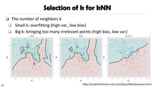
Selection of k for kNN
❑ The number of neighbors k
❑ Small k: overfitting (high var., low bias)
❑ Big k: bringing too many irrelevant points (high bias, low var.)
http://scott.fortmann-roe.com/docs/BiasVariance.html

38
Case-Based Reasoning (CBR)
❑ CBR: Uses a database of problem solutions to solve new problems
❑ Store symbolic description (tuples or cases)—not points in a Euclidean space
❑ Applications: Customer-service (product-related diagnosis), legal ruling
❑ Methodology
❑ Instances represented by rich symbolic descriptions (e.g., function graphs)
❑ Search for similar cases, multiple retrieved cases may be combined
❑ Tight coupling between case retrieval, knowledge-based reasoning, and problem
solving
❑ Challenges
❑ Find a good similarity metric
❑ Indexing based on syntactic similarity measure, and when failure, backtracking,
and adapting to additional cases

39
❑ Summary

40
Linear Regression Problem: Example
❑ Mapping from independent attributes to continuous value: x => y
❑ {living area} => Price of the house
❑ {college; major; GPA} => Future Income
Price
of
houses
Living Area

41
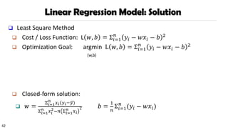
Linear Regression Problem: Model
❑ Linear regression
❑ Data: n independent objects
❑ Observed Value: 𝑦𝑖, 𝑖 = 1,2,3, ⋯ , 𝑛
❑ p-dimensional attributes: 𝑥𝑖 = 𝑥𝑖1, 𝑥𝑖2, ⋯ , 𝑥𝑖𝑝
𝑇
, 𝑖 = 1,2,3 ⋯ , 𝑛
❑ Model:
❑ Weight vector: 𝑤 = 𝑤1, 𝑤2, ⋯ , 𝑤𝑝
❑ 𝑦𝑖 = 𝑤𝑇𝑥𝑖 + 𝑏
❑ The weight vector w and bias b are the model parameter learnt by data

42
Linear Regression Model: Solution
❑ Least Square Method
❑ Cost / Loss Function: L 𝑤, 𝑏 = Σ𝑖=1
𝑛
𝑦𝑖 − 𝑤𝑥𝑖 − 𝑏 2
❑ Optimization Goal: argmin L 𝑤, 𝑏 = Σ𝑖=1
𝑛
𝑦𝑖 − 𝑤𝑥𝑖 − 𝑏 2
❑ Closed-form solution:
❑ 𝑤 =
Σ𝑖=1
𝑛
𝑥𝑖(𝑦𝑖− ത
𝑦)
Σ𝑖=1
𝑛 𝑥𝑖
2−𝑛 Σ𝑖=1
𝑛 𝑥𝑖
2 𝑏 =
1
𝑛
Σ𝑖=1
𝑛
(𝑦𝑖 − 𝑤𝑥𝑖)
(w,b)

43
Logistic Regression: General Ideas
❑ How to solve “classification” problems by regression?
❑ Key idea of Logistic Regression
❑ We need to transform the real value Y into a probability value ∈ [0,1]
❑ Sigmoid function (differentiable function) :
❑ 𝜎 𝑧 =
1
1+𝑒−𝑧 =
𝑒𝑧
𝑒𝑧+1
❑ Projects (−∞, +∞) to [0, 1]
❑ Not only LR uses this function, but also
neural network, deep learning
❑ The projected value changes sharply
around zero point
❑ Notice that ln
y
1−𝑦
= 𝑤𝑇𝑥 + 𝑏
Sigmoid
Function

44
Logistic Regression: An Example
❑ Suppose we only consider the year as feature
❑ Data points are converted by sigmoid function (“activation” function)
year
6
1 (Tenured)

45
Logistic Regression: Model
❑ The prediction function to learn
❑ Probability that Y=1:
❑ 𝑝 𝑌 = 1 𝑋 = 𝑥; 𝒘) = 𝑆𝑖𝑔𝑚𝑜𝑖𝑑 𝑤0 + σ𝑖=1
𝑛
𝑤𝑖 ⋅ 𝑥𝑖
❑ 𝒘 = 𝑤0, 𝑤1, 𝑤2, … , 𝑤𝑛 are the parameters
❑ A single data object with attributes 𝑥𝑖 and class label 𝑦𝑖
❑ Suppose the probability of 𝑝 ෝ
𝑦𝑖 = 1 𝑥𝑖, 𝑤 = 𝑝𝑖, then 𝑝 ෝ
𝑦𝑖 = 0 𝑥𝑖, 𝑤 = 1 − 𝑝𝑖
❑ 𝑝 ෝ
𝑦𝑖 = 𝑦𝑖 = 𝑝𝑖
𝑦𝑖
1 − 𝑝𝑖
1−𝑦𝑖
❑ Maximum Likelihood Estimation
❑ 𝐿 = Π𝑖𝑝𝑖
𝑦𝑖
1 − 𝑝𝑖
1−𝑦𝑖 = Π𝑖
exp 𝑤𝑇𝑥𝑖
1+exp 𝑤𝑇𝑥𝑖
𝑦𝑖
1
1−𝑦𝑖

46
Logistic Regression: Optimization
❑ Maximum Likelihood Estimation
❑ 𝐿 = Π𝑖𝑝𝑖
𝑦𝑖
1 − 𝑝𝑖
1−𝑦𝑖 = Π𝑖
exp 𝑤𝑇𝑥𝑖
𝑦𝑖
1
1−𝑦𝑖
❑ Log likelihood:
𝑙 𝑤 = ෍
𝑖=1
𝑁
𝑦𝑖 log 𝑝 𝑌 = 1 𝑋 = 𝑥𝑖; 𝒘 + 1 − 𝑦𝑖 log 1 − 𝑝 𝑌 = 1 𝑋 = 𝑥𝑖; 𝒘
= ෍
𝑖=1
𝑁
𝑦𝑖𝑥𝑖
𝑇
𝒘 − log(1 + exp 𝒘𝑇𝑥𝑖 )
❑ There’s no closed form solution
❑ Gradient Descent/Ascent

47
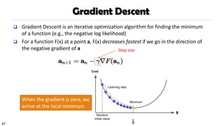
Gradient Descent
❑ Gradient Descent is an iterative optimization algorithm for finding the minimum
of a function (e.g., the negative log likelihood)
❑ For a function F(x) at a point a, F(x) decreases fastest if we go in the direction of
the negative gradient of a
When the gradient is zero, we
arrive at the local minimum
Step size

48
Gradient Descent
[footnote: It is gradient ascent for maximizing log likelihood]
Note we have switched the index i in the previous slides to l, and use i to refer to different components of weight vector w

49
Gradient Descent

50
Gradient Descent

51
❑ Summary

52
Model Evaluation and Selection
❑ Evaluation metrics
❑ How can we measure accuracy?
❑ Other metrics to consider?
❑ Use validation test set of class-labeled tuples instead of training set when assessing
accuracy
❑ Methods for estimating a classifier’s accuracy
❑ Holdout method
❑ Cross-validation
❑ Bootstrap (not covered)
❑ Comparing classifiers:
❑ ROC Curves

53
Classifier Evaluation Metrics: Confusion Matrix
Actual classPredicted class play_golf = yes play_golf = no Total
play_golf = yes 6954 46 7000
play_golf = no 412 2588 3000
Total 7366 2634 10000
❑ Confusion Matrix:
❑ In a confusion matrix w. m classes, CMi,j indicates # of tuples in class i that
were labeled by the classifier as class j
❑ May have extra rows/columns to provide totals
❑ Example of Confusion Matrix:
Actual classPredicted class C1 ¬ C1
C1 True Positives (TP) False Negatives (FN)
¬ C1 False Positives (FP) True Negatives (TN)

54
Classifier Evaluation Metrics: Accuracy, Error Rate,
Sensitivity and Specificity
❑ Classifier accuracy, or
recognition rate
❑ Percentage of test set tuples
that are correctly classified
Accuracy = (TP + TN)/All
❑ Error rate: 1 – accuracy, or
Error rate = (FP + FN)/All
AP C ¬C
C TP FN P
¬C FP TN N
P’ N’ All
❑ Class imbalance problem
❑ One class may be rare
❑ E.g., fraud, or HIV-positive
❑ Significant majority of the negative class and
minority of the positive class
❑ Measures handle the class imbalance problem
❑ Sensitivity (recall): True positive recognition
rate
❑ Sensitivity = TP/P
❑ Specificity: True negative recognition rate
❑ Specificity = TN/N
Real-world
truth
Predictions

55
Classifier Evaluation Metrics:
Precision and Recall, and F-measures
❑ Precision: Exactness: what % of tuples that the
classifier labeled as positive are actually positive?
❑ Recall: Completeness: what % of positive tuples did
the classifier label as positive?
❑ Range: [0, 1]
P = Precision =
TP
TP + FP
R = Recall =
TP
TP + FN
https://en.wikipedia.org/wiki/Precision_and_recall
AP C ¬C
C TP FN P
¬C FP TN N
P’ N’ All

56
Classifier Evaluation Metrics:
Precision and Recall, and F-measures
❑ The “inverse” relationship between precision & recall
❑ We want one number to say if a classifier is good or not
❑ F measure (or F-score): harmonic mean of precision and recall
❑ In general, it is the weighted measure of precision & recall
❑ F1-measure (balanced F-measure)
❑ That is, when β = 1,
Assigning β times as much
weight to recall as to precision
F𝛽 =
1
𝛼 ∙
1
P
+ (1 − 𝛼) ∙
1
R
=
β2 + 1 P ∗ R
β2P + R
F1 =
2P ∗ R
P + R

57
Classifier Evaluation Metrics: Example
Actual ClassPredicted class cancer = yes cancer = no Total
cancer = yes 90 210 300
cancer = no 140 9560 9700
Total 230 9770 10000
❑ Use the same confusion matrix, calculate the measure just introduced
❑ Sensitivity =
❑ Specificity =
❑ Accuracy =
❑ Error rate =
❑ Precision =
❑ Recall =
❑ F1 =

58
Classifier Evaluation Metrics: Example
Actual ClassPredicted class cancer = yes cancer = no Total
cancer = yes 90 210 300
cancer = no 140 9560 9700
Total 230 9770 10000
❑ Use the same confusion matrix, calculate the measure just introduced
❑ Sensitivity = TP/P = 90/300 = 30%
❑ Specificity = TN/N = 9560/9700 = 98.56%
❑ Accuracy = (TP + TN)/All = (90+9560)/10000 = 96.50%
❑ Error rate = (FP + FN)/All = (140 + 210)/10000 = 3.50%
❑ Precision = TP/(TP + FP) = 90/(90 + 140) = 90/230 = 39.13%
❑ Recall = TP/ (TP + FN) = 90/(90 + 210) = 90/300 = 30.00%
❑ F1 = 2 P × R /(P + R) = 2 × 39.13% × 30.00%/(39.13% + 30%) = 33.96%

59
Training Error VS Testing Error
59
overfitting
underfitting

60
Classifier Evaluation: Holdout
❑ Holdout method
❑ Given data is randomly partitioned into two independent sets
❑ Training set (e.g., 2/3) for model construction
❑ Test set (e.g., 1/3) for accuracy estimation
❑ Repeated random sub-sampling validation: a variation of holdout
❑ Repeat holdout k times, accuracy = avg. of the accuracies obtained

61
Classifier Evaluation: Cross-Validation
❑ Cross-validation (k-fold, where k = 10 is most popular)
❑ Randomly partition the data into k mutually exclusive subsets, each
approximately equal size
❑ At i-th iteration, use Di as test set and others as training set
❑ Leave-one-out: k folds where k = # of tuples, for small sized data
❑ *Stratified cross-validation*: folds are stratified so that class
distribution, in each fold is approximately the same as that in the
initial data

62
Model Selection: ROC Curves
❑ ROC (Receiver Operating Characteristics) curves:
for visual comparison of classification models
❑ Originated from signal detection theory
❑ Shows the trade-off between the true positive
rate and the false positive rate
❑ The area under the ROC curve (AUC: Area Under
Curve) is a measure of the accuracy of the model
❑ Rank the test tuples in decreasing order: the one
that is most likely to belong to the positive class
appears at the top of the list
❑ The closer to the diagonal line (i.e., the closer the
area is to 0.5), the less accurate is the model
❑ Vertical axis represents the
true positive rate (TP/P)
❑ Horizontal axis rep. the false
positive rate (FP/N)
❑ The plot also shows a diagonal
line
❑ A model with perfect accuracy
will have an area of 1.0
False positive rate
True
positive
rate

63
❑ Summary

64
Techniques to Improve Classification Accuracy
❑ Introducing Ensemble Methods
❑ Bagging
❑ Boosting
❑ Random Forests
❑ Imbalanced Classification

65
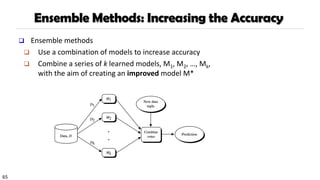
Ensemble Methods: Increasing the Accuracy
❑ Ensemble methods
❑ Use a combination of models to increase accuracy
❑ Combine a series of k learned models, M1, M2, …, Mk,
with the aim of creating an improved model M*

66
❑ What are the requirements to generate an improved model?
❑ Example: majority voting
x1 x2 x3
M1 ✓ ✓ ✗
M2 ✗ ✓ ✓
M3 ✓ ✗ ✓
Voting
Ensemble
✓ ✓ ✓
x1 x2 x3
M1 ✓ ✓ ✗
M2 ✓ ✓ ✗
M3 ✓ ✓ ✗
Voting
Ensemble
✓ ✓ ✗
x1 x2 x3
M1 ✓ ✗ ✗
M2 ✗ ✓ ✗
M3 ✗ ✗ ✓
Voting
Ensemble
✗ ✗ ✗
Base model
performance
Ensemble
performance
Case 1:
Ensemble has positive effect
Case 2:
Ensemble has no effect
Case 3:
Ensemble has negative effect
❑ Base models should be
❑ Accurate
❑ Diverse

67
❑ Popular ensemble methods
❑ Bagging: Trains each model using a subset of the training set, and models
learned in parallel
❑ Boosting: Trains each new model instance to emphasize the training instances
that previous models mis-classified, and models learned in order
Bagging Boosting

68
Bagging: Bootstrap Aggregation
❑ Analogy: Diagnosis based on multiple doctors’ majority vote
❑ Training
❑ For i = 1 to k
❑ create bootstrap sample, Di, by sampling D with replacement;
❑ use Di and the learning scheme to derive a model, Mi ;
❑ Classification: classify an unknown sample X
❑ let each of the k models classify X and return the majority vote
❑ Prediction:
❑ To predict continuous variables, use average prediction instead of vote

69
Boosting
❑ Analogy: Consult several doctors, based on a combination of weighted diagnoses—
weight assigned based on the previous diagnosis accuracy
❑ How boosting works?
❑ A series of k classifiers are iteratively learned
❑ After a classifier Mi is learned, set the subsequent classifier, Mi+1, to pay more
attention to the training tuples that were misclassified by Mi
❑ The final M* combines the votes of each individual classifier, where the weight
of each classifier's vote is a function of its accuracy
❑ Boosting algorithm can be extended for numeric prediction

70
Adaboost (Freund and Schapire, 1997)
{wn
(1)} {wn
(2)} {wn
(k)}
M1 M2 Mk
…
…
𝑀∗
𝑥 = sign ෍
𝑖=1
𝑘
𝛼𝑖𝑀𝑖 𝑥
1. Assign initial
weights to each
training tuple
2. Train base
classifier on
weighted dataset
3. Update weights
based on current
model
4. After base classifiers
are trained, they are
combined to give the
final classifier
Two ‘weighting’ strategy:
1. Assign weights to each training
example
2. Sample dataset based on weight
distribution

71
Adaboost (Freund and Schapire, 1997)
❑ Input: Training set 𝐷 = 𝑥1, 𝑦1 , 𝑥2, 𝑦2 , … , 𝑥𝑛, 𝑦𝑛
❑ Initialize all weights {𝑤𝑛
1
} to 1/N
❑ For round i = 1 to k,
❑ Fit a classifier 𝑀𝑖 based on weighted error function
𝐽𝑚 = ෍
𝑛=1
𝑁
𝑤𝑛
𝑖
𝐼 𝑀𝑖 𝑥𝑛 ≠ 𝑦𝑛
❑ Evaluate error rate 𝜖𝑖 = 𝐽𝑚/ σ 𝑤𝑛
𝑖
(stop iteration if 𝜖𝑖 < threshold)
and the base model 𝑀𝑖’s vote 𝛼𝑖 =
1
2
ln
1−𝜖𝑖
𝜖𝑖
❑ Update weights
𝑤𝑛
(𝑖+1)
= 𝑤𝑛
(𝑖)
exp{𝛼𝑖 ⋅ 𝐼 𝑀𝑖 𝑥𝑛 ≠ 𝑦𝑛 }
❑ The final model is given by voting based on {𝛼𝑛}

72
Gradient Boosting
❑ Operates on:
❑ A differentiable loss function
❑ A weak learner to make predictions (usually trees)
❑ An additive model to add weak learners to minimize the loss function
❑ Each time adds an additional weak learner
❑ Scalable implementation: XGBoost
Previous model
New weak learner

73
Random Forest: Basic Concepts
❑ Random Forest (first proposed by L. Breiman in 2001)
❑ Bagging with decision trees as base models
❑ Data bagging
❑ Use a subset of training data by sampling with replacement for each tree
❑ Feature bagging
❑ At each node use a random selection of attributes as candidates and split by
the best attribute among them
❑ During classification, each tree votes and the most popular class is returned
Advantage of decision trees – more diversity

74
Random Forest
❑ Two Methods to construct Random Forest:
❑ Forest-RI (random input selection): Randomly select, at each node, F attributes
as candidates for the split at the node. The CART methodology is used to grow
the trees to maximum size
❑ Forest-RC (random linear combinations): Creates new attributes (or features)
that are a linear combination of the existing attributes (reduces the correlation
between individual classifiers)
❑ Comparable in accuracy to Adaboost, but more robust to errors and outliers
❑ Insensitive to the number of attributes selected for consideration at each split, and
faster than typical bagging or boosting

75
Ensemble Methods Recap
❑ Random forest and XGBoost are the most commonly used algorithms for tabular data
❑ Pros
❑ Good performance for tabular data, requires no data scaling
❑ Can scale to large datasets
❑ Can handle missing data to some extent
❑ Cons
❑ Can overfit to training data if not tuned properly
❑ Lack of interpretability (compared to decision trees)

76
Classification of Class-Imbalanced Data Sets
❑ Traditional methods assume a balanced distribution of classes and equal error
costs. But in real world situations, we may face imbalanced data sets, which has
rare positive examples but numerous negative ones.
❑ Medical diagnosis: Medical screening for a condition
is usually performed on a large population of people
without the condition, to detect a small minority
with it (e.g., HIV prevalence in the USA is ~0.4%)
❑ Fraud detection: About 2% of credit card accounts
are defrauded per year. (Most fraud detection domains are heavily imbalanced.)
❑ Product defect, accident (oil-spill), disk drive failures, etc.

77
❑ Typical methods on imbalanced data (Balance the training set)
❑ Oversampling: Oversample the minority class.
❑ Under-sampling: Randomly eliminate tuples from majority class
❑ Synthesizing: Synthesize new minority classes

78
❑ Typical methods on imbalanced data (At the algorithm level)
❑ Threshold-moving: Move the decision threshold, t, so that the rare class tuples
are easier to classify, and hence, less chance of costly false negative errors
❑ Class weight adjusting: Since false negative costs more than false positive, we
can give larger weight to false negative
❑ Ensemble techniques: Ensemble multiple classifiers introduced in the following
chapter
Threshold-
moving

79
Evaluate imbalanced data classifier
❑ Can we use Accuracy to evaluate imbalanced data classifier?
❑ Accuracy simply counts the number of errors. If a data set has 2% positive
labels and 98% negative labels, a classifier that map all inputs to negative
class will get an accuracy of 98%!
❑ ROC Curve

80
Summary
❑ Classification: Model construction from a set of training data
❑ Effective and scalable methods
❑ Decision tree induction, Bayes classification methods, lazy learners, linear classifier
❑ No single method has been found to be superior over all others for all data sets
❑ Evaluation metrics: Accuracy, sensitivity, specificity, precision, recall, F measure
❑ Model evaluation: Holdout, cross-validation, bootstrapping, ROC curves (AUC)
❑ Techniques to improve classification accuracy: Ensemble Methods (bagging, boosting,
random forests), imbalanced classification

81
References (1)
❑ C. Apte and S. Weiss. Data mining with decision trees and decision rules. Future
Generation Computer Systems, 13, 1997
❑ A. J. Dobson. An Introduction to Generalized Linear Models. Chapman & Hall, 1990.
❑ R. O. Duda, P. E. Hart, and D. G. Stork. Pattern Classification, 2ed. John Wiley, 2001
❑ U. M. Fayyad. Branching on attribute values in decision tree generation. AAAI’94.
❑ Y. Freund and R. E. Schapire. A decision-theoretic generalization of on-line learning and
an application to boosting. J. Computer and System Sciences, 1997.
❑ J. Gehrke, R. Ramakrishnan, and V. Ganti. Rainforest: A framework for fast decision tree
construction of large datasets. VLDB’98.
❑ J. Gehrke, V. Gant, R. Ramakrishnan, and W.-Y. Loh, BOAT -- Optimistic Decision Tree
Construction. SIGMOD'99.
❑ T. Hastie, R. Tibshirani, and J. Friedman. The Elements of Statistical Learning: Data
Mining, Inference, and Prediction. Springer-Verlag, 2001
❑ J. Pan and D. Manocha. Bi-level locality sensitive hashing for k-nearest neighbor
computation. IEEE ICDE 2012

82
References (2)
❑ T.-S. Lim, W.-Y. Loh, and Y.-S. Shih. A comparison of prediction accuracy, complexity, and
training time of thirty-three old and new classification algorithms. Machine Learning, 2000
❑ J. Magidson. The Chaid approach to segmentation modeling: Chi-squared automatic
interaction detection. In R. P. Bagozzi, editor, Advanced Methods of Marketing Research,
Blackwell Business, 1994
❑ M. Mehta, R. Agrawal, and J. Rissanen. SLIQ : A fast scalable classifier for data mining. EDBT'96
❑ T. M. Mitchell. Machine Learning. McGraw Hill, 1997
❑ S. K. Murthy, Automatic Construction of Decision Trees from Data: A Multi-Disciplinary Survey,
Data Mining and Knowledge Discovery 2(4): 345-389, 1998
❑ J. R. Quinlan. Induction of decision trees. Machine Learning, 1:81-106, 1986
❑ J. R. Quinlan. C4.5: Programs for Machine Learning. Morgan Kaufmann, 1993
❑ J. R. Quinlan. Bagging, boosting, and c4.5. AAAI’96
❑ E. Alpaydin. Introduction to Machine Learning (2nd ed.). MIT Press, 2011

83
References (3)
❑ R. Rastogi and K. Shim. Public: A decision tree classifier that integrates building and
pruning. VLDB’98
❑ J. Shafer, R. Agrawal, and M. Mehta. SPRINT : A scalable parallel classifier for data
mining. VLDB’96
❑ J. W. Shavlik and T. G. Dietterich. Readings in Machine Learning. Morgan Kaufmann, 1990
❑ P. Tan, M. Steinbach, and V. Kumar. Introduction to Data Mining. Addison Wesley, 2005
❑ S. M. Weiss and C. A. Kulikowski. Computer Systems that Learn: Classification and
Prediction Methods from Statistics, Neural Nets, Machine Learning, and Expert Systems.
Morgan Kaufman, 1991
❑ S. M. Weiss and N. Indurkhya. Predictive Data Mining. Morgan Kaufmann, 1997
❑ I. H. Witten and E. Frank. Data Mining: Practical Machine Learning Tools and Techniques,
2ed. Morgan Kaufmann, 2005
❑ T. Chen and C. Guestrin. Xgboost: A Scalable Tree Boosting System. ACM SIGKDD 2016
❑ C. Aggarwal. Data Classication. Morgan Springer, 2015

Chap6-ClassificationBasic_data_mining.pdf

More Related Content

Similar to Chap6-ClassificationBasic_data_mining.pdf

More from SaifUddin617640

Recently uploaded

Chap6-ClassificationBasic_data_mining.pdf