This document contains 32 numerical problems related to time value of money concepts. Some key details summarized:
- Problem 1 calculates future values over 5 years at interest rates of 8%, 10%, 12%, and 15%.
- Problem 15 uses linear interpolation to find an implied interest rate of 15.1% between given values.
- Problem 32 calculates the present value of expected iron ore mining revenues over 15 years, discounting for price escalation of 6% annually.

![PVIF (12%, 4 years) + Rs.500 x PVIF (12%, 5 years) +
Rs.600 x PVIF (12%, 6 years) + Rs.700 x PVIF (12%, 7 years) +
Rs.800 x PVIF (12%, 8 years) + Rs.900 x PVIF (12%, 9 years) +
Rs.1,000 x PVIF (12%, 10 years)
= Rs.100 x 0.893 + Rs.200 x 0.797 + Rs.300 x 0.712
+ Rs.400 x 0.636 + Rs.500 x 0.567 + Rs.600 x 0.507
+ Rs.700 x 0.452 + Rs.800 x 0.404 + Rs.900 x 0.361
+ Rs.1,000 x 0.322
= Rs.2590.9
Similarly,
PV (Stream B) = Rs.3,625.2
PV (Stream C) = Rs.2,851.1
17. FV5 = Rs.10,000 [1 + (0.16 / 4)]5x4
= Rs.10,000 (1.04)20
= Rs.10,000 x 2.191
= Rs.21,910
18. FV5 = Rs.5,000 [1+( 0.12/4)] 5x4
= Rs.5,000 (1.03)20
= Rs.5,000 x 1.806
= Rs.9,030
19 A B C
Stated rate (%) 12 24 24
Frequency of compounding 6 times 4 times 12 times
Effective rate (%) (1 + 0.12/6)6
- 1 (1+0.24/4)4
–1 (1 + 0.24/12)12
-1
= 12.6 = 26.2 = 26.8
Difference between the
effective rate and stated
rate (%) 0.6 2.2 2.8
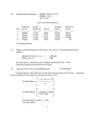
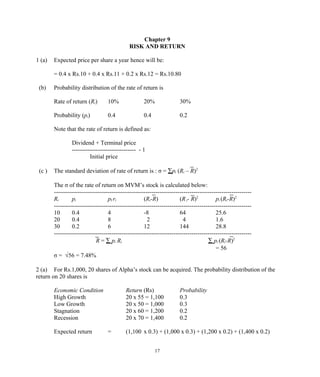
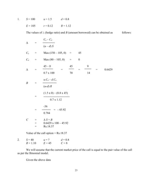
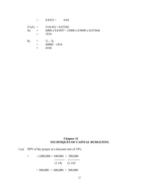
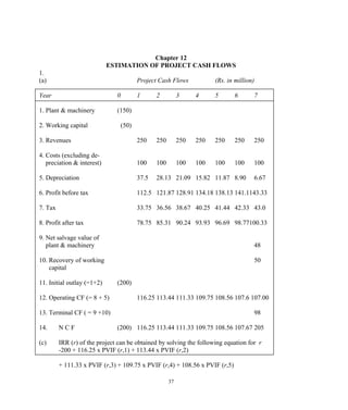
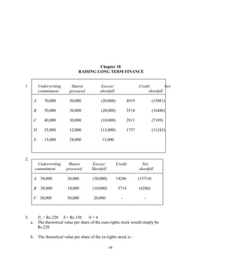
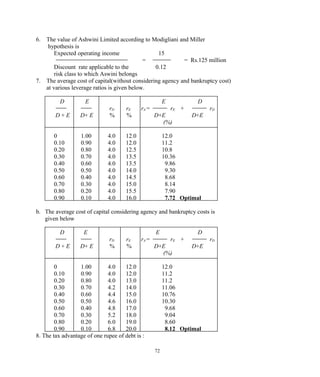
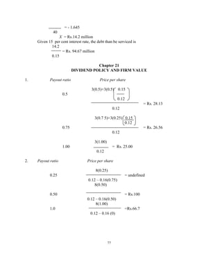
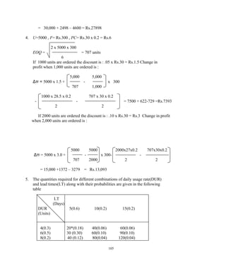
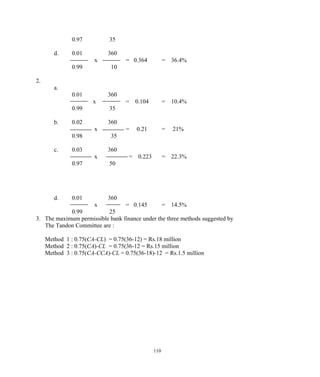
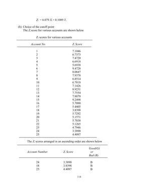
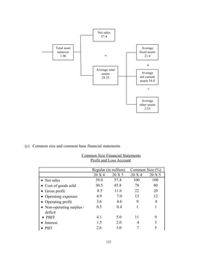
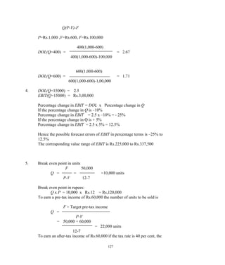
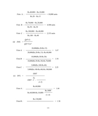
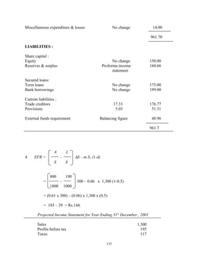
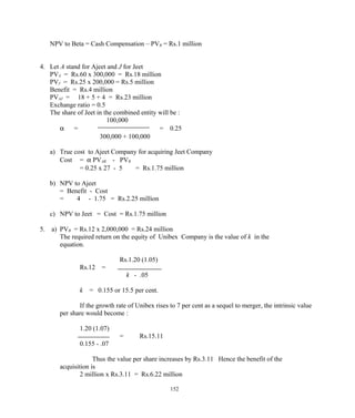
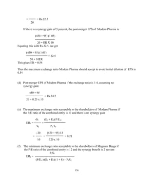
20. Investment required at the end of 8th
year to yield an income of Rs.12,000 per year from the
end of 9th
year (beginning of 10th
year) for ever:
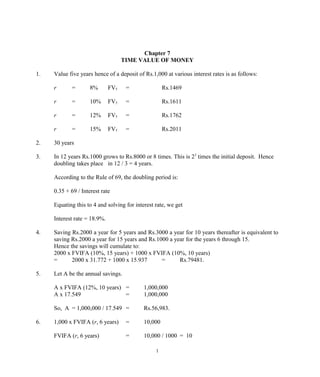
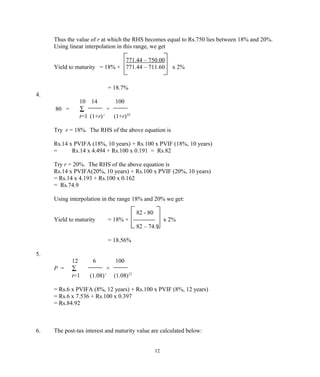
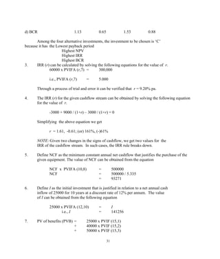
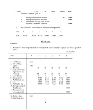
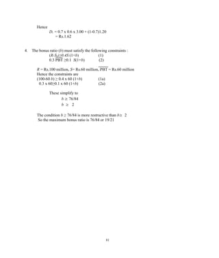
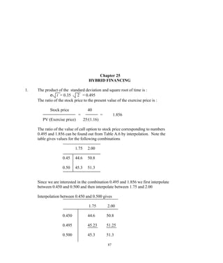
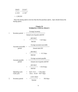
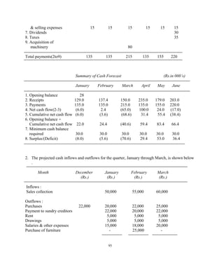
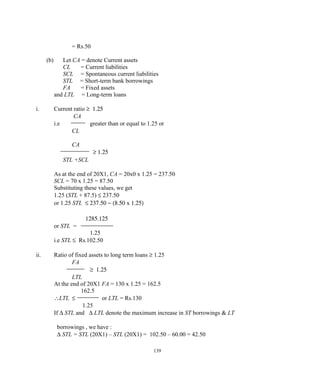
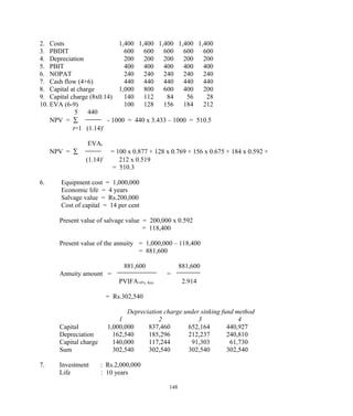
Rs.12,000 x PVIFA(12%, ∞ )
4](https://image.slidesharecdn.com/199776069-prasanna-chandra-financial-management-220826060839-ab52aacb/85/199776069-prasanna-chandra-financial-management-pdf-4-320.jpg)
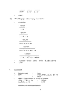
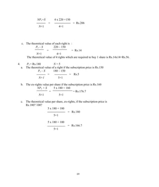
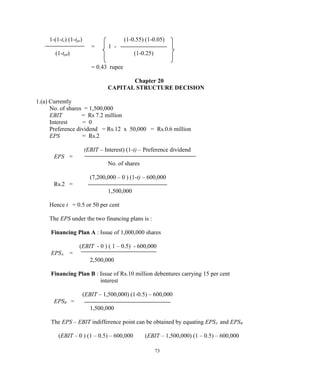
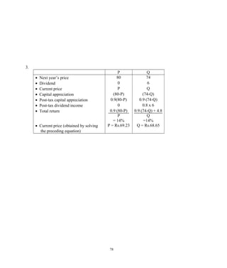
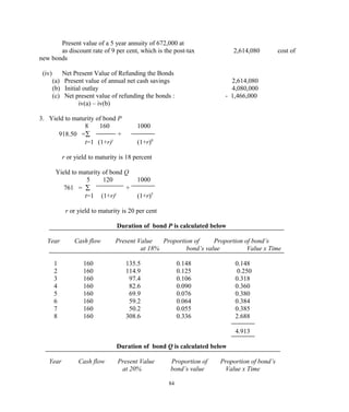
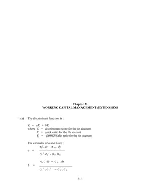
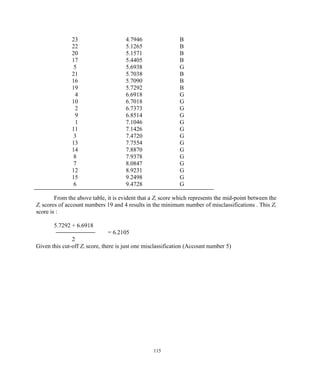
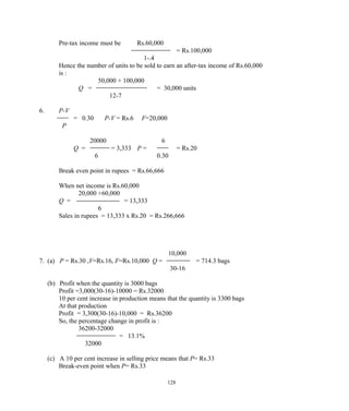
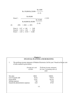
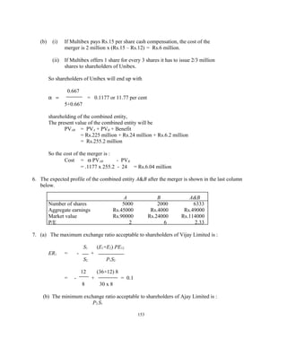
![= Rs.12,000 / 0.12 = Rs.100,000
To have a sum of Rs.100,000 at the end of 8th
year , the amount to be deposited now is:
Rs.100,000 Rs.100,000
= = Rs.40,388
PVIF(12%, 8 years) 2.476
21. The interest rate implicit in the offer of Rs.20,000 after 10 years in lieu of Rs.5,000 now is:
Rs.5,000 x FVIF (r,10 years) = Rs.20,000
Rs.20,000
FVIF (r,10 years) = = 4.000
Rs.5,000
From the tables we find that
FVIF (15%, 10 years) = 4.046
This means that the implied interest rate is nearly 15%.
I would choose Rs.20,000 for 10 years from now because I find a return of 15% quite
acceptable.
22. FV10 = Rs.10,000 [1 + (0.10 / 2)]10x2
= Rs.10,000 (1.05)20
= Rs.10,000 x 2.653
= Rs.26,530
If the inflation rate is 8% per year, the value of Rs.26,530 10 years from now, in terms of
the current rupees is:
Rs.26,530 x PVIF (8%,10 years)
= Rs.26,530 x 0.463 = Rs.12,283
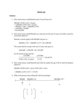
23. A constant deposit at the beginning of each year represents an annuity due.
PVIFA of an annuity due is equal to : PVIFA of an ordinary annuity x (1 + r)
To provide a sum of Rs.50,000 at the end of 10 years the annual deposit should
be
Rs.50,000
A = FVIFA(12%, 10 years) x (1.12)
Rs.50,000
= = Rs.2544
17.549 x 1.12
5](https://image.slidesharecdn.com/199776069-prasanna-chandra-financial-management-220826060839-ab52aacb/85/199776069-prasanna-chandra-financial-management-pdf-5-320.jpg)
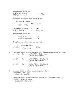
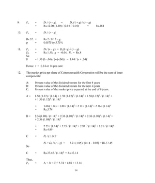
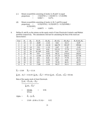
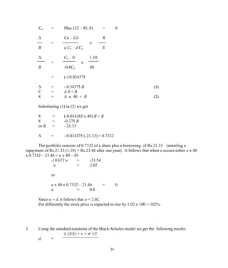
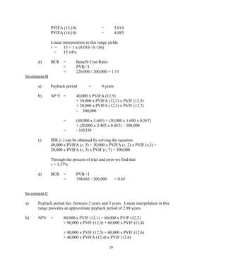
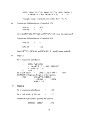
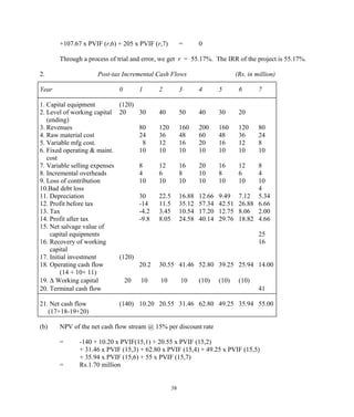
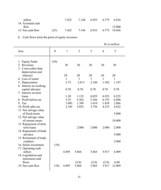
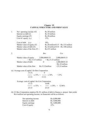
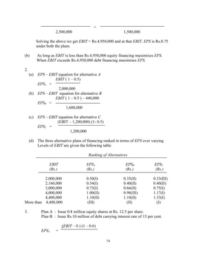
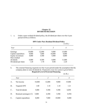
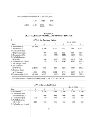
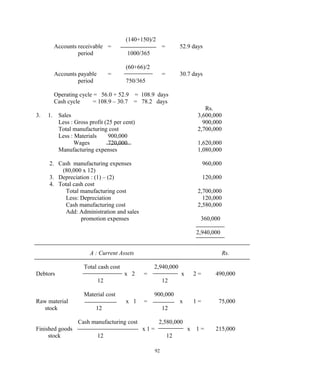
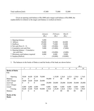
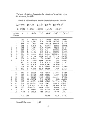
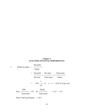
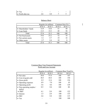
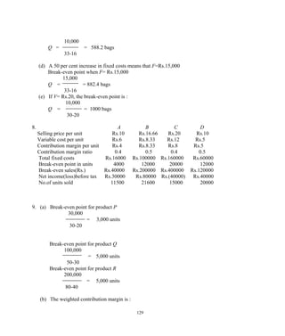
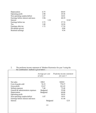
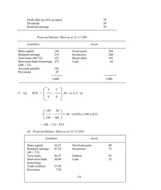
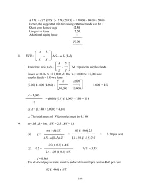
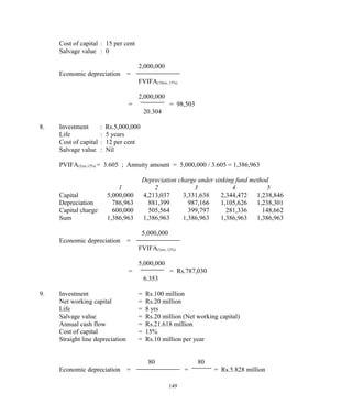
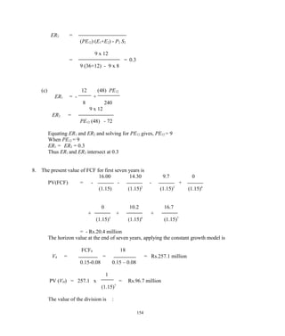
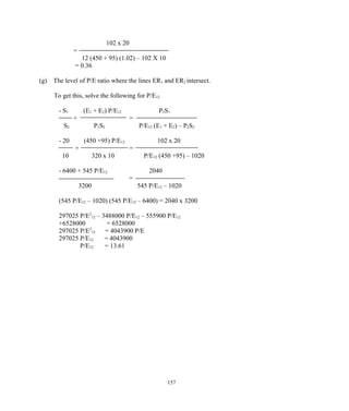
![PVIFA (2%, 24) = 18.914
Using a linear interpolation
21.244 – 20.000
r = 1% + ---------------------- x 1%
21.244 – 18,914
= 1.53%
Thus, the bank charges an interest rate of 1.53% per month.
The corresponding effective rate of interest per annum is
[ (1.0153)12
– 1 ] x 100 = 20%
28. The discounted value of the debentures to be redeemed between 8 to 10 years evaluated at
the end of the 5th
year is:
Rs.10 million x PVIF (8%, 3 years)
+ Rs.10 million x PVIF (8%, 4 years)
+ Rs.10 million x PVIF (8%, 5 years)
= Rs.10 million (0.794 + 0.735 + 0.681)
= Rs.2.21 million
If A is the annual deposit to be made in the sinking fund for the years 1 to 5,
then
A x FVIFA (8%, 5 years) = Rs.2.21 million
A x 5.867 = Rs.2.21 million
A = 5.867 = Rs.2.21 million
A = Rs.2.21 million / 5.867 = Rs.0.377 million
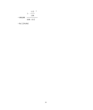
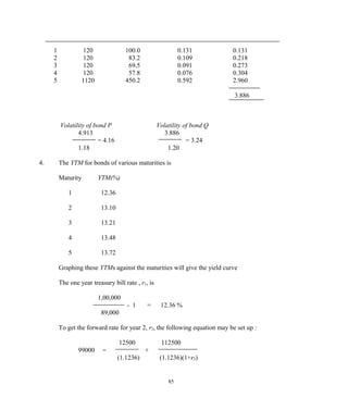
29. Let `n’ be the number of years for which a sum of Rs.20,000 can be withdrawn annually.
Rs.20,000 x PVIFA (10%, n) = Rs.100,000
PVIFA (15%, n) = Rs.100,000 / Rs.20,000 = 5.000
From the tables we find that
PVIFA (10%, 7 years) = 4.868
PVIFA (10%, 8 years) = 5.335
Thus n is between 7 and 8. Using a linear interpolation we get
5.000 – 4.868
n = 7 + ----------------- x 1 = 7.3 years
5.335 – 4.868
7](https://image.slidesharecdn.com/199776069-prasanna-chandra-financial-management-220826060839-ab52aacb/85/199776069-prasanna-chandra-financial-management-pdf-7-320.jpg)
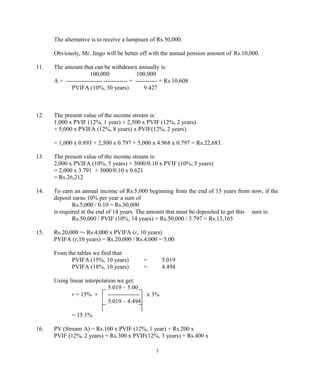
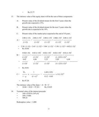
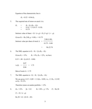
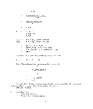
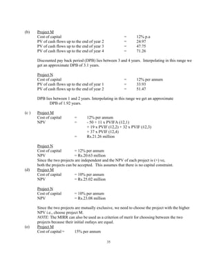
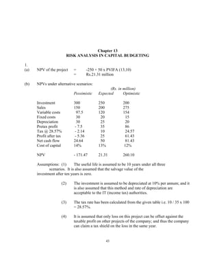
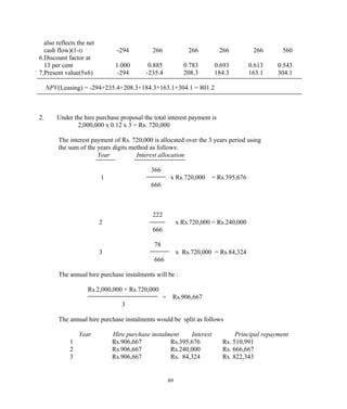
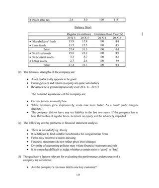
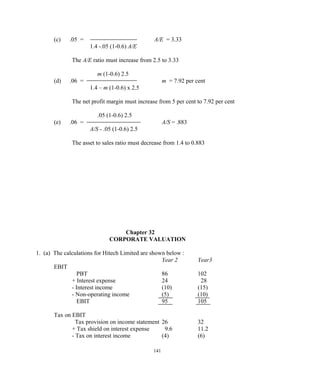
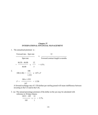
![Bond A Bond B
* Post-tax interest (C ) 12(1 – 0.3) 10 (1 – 0.3)
=Rs.8.4 =Rs.7
* Post-tax maturity value (M) 100 - 100 -
[ (100-70)x 0.1] [ (100 – 60)x 0.1]
=Rs.97 =Rs.96
The post-tax YTM, using the approximate YTM formula is calculated below
8.4 + (97-70)/10
Bond A : Post-tax YTM = --------------------
0.6 x 70 + 0.4 x 97
= 13.73%
7 + (96 – 60)/6
Bond B : Post-tax YTM = ----------------------
0.6x 60 + 0.4 x 96
= 17. 47%
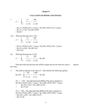
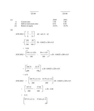
7.
14 6 100
P = ∑ +
t=1 (1.08) t
(1.08)14
= Rs.6 x PVIFA(8%, 14) + Rs.100 x PVIF (8%, 14)
= Rs.6 x 8.244 + Rs.100 x 0.341
= Rs.83.56
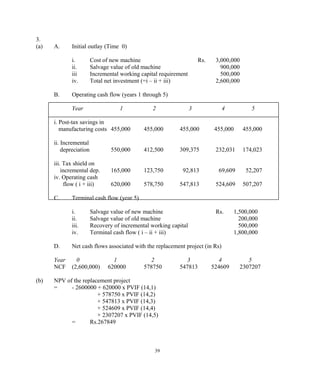
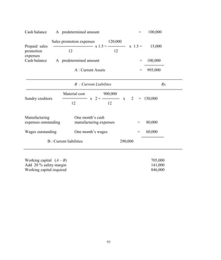
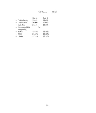
8. Do = Rs.2.00, g = 0.06, r = 0.12
Po = D1 / (r – g) = Do (1 + g) / (r – g)
= Rs.2.00 (1.06) / (0.12 - 0.06)
= Rs.35.33
Since the growth rate of 6% applies to dividends as well as market price, the market
price at the end of the 2nd
year will be:
P2 = Po x (1 + g)2
= Rs.35.33 (1.06)2
= Rs.39.70
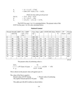
13](https://image.slidesharecdn.com/199776069-prasanna-chandra-financial-management-220826060839-ab52aacb/85/199776069-prasanna-chandra-financial-management-pdf-13-320.jpg)
![= 330 + 300 + 240 + 280
= Rs.1,150
Standard deviation of the return = [(1,100 – 1,150)2
x 0.3 + (1,000 – 1,150)2
x
0.3 + (1,200 – 1,150)2
x 0.2 + (1,400 – 1,150)2
x 0.2]1/2
= Rs.143.18
(b) For Rs.1,000, 20 shares of Beta’s stock can be acquired. The probability distribution of the
return on 20 shares is:
Economic condition Return (Rs) Probability
High growth 20 x 75 = 1,500 0.3
Low growth 20 x 65 = 1,300 0.3
Stagnation 20 x 50 = 1,000 0.2
Recession 20 x 40 = 800 0.2
Expected return = (1,500 x 0.3) + (1,300 x 0.3) + (1,000 x 0.2) + (800 x 0.2)
= Rs.1,200
Standard deviation of the return = [(1,500 – 1,200)2
x .3 + (1,300 – 1,200)2
x .3
+ (1,000 – 1,200)2
x .2 + (800 – 1,200)2
x .2]1/2
= Rs.264.58
(c ) For Rs.500, 10 shares of Alpha’s stock can be acquired; likewise for Rs.500, 10
shares of Beta’s stock can be acquired. The probability distribution of this option is:
Return (Rs) Probability
(10 x 55) + (10 x 75) = 1,300 0.3
(10 x 50) + (10 x 65) = 1,150 0.3
(10 x 60) + (10 x 50) = 1,100 0.2
(10 x 70) + (10 x 40) = 1,100 0.2
Expected return = (1,300 x 0.3) + (1,150 x 0.3) + (1,100 x 0.2) +
(1,100 x 0.2)
= Rs.1,175
Standard deviation = [(1,300 –1,175)2
x 0.3 + (1,150 – 1,175)2
x 0.3 +
(1,100 – 1,175)2
x 0.2 + (1,100 – 1,175)2
x 0.2 ]1/2
= Rs.84.41
d. For Rs.700, 14 shares of Alpha’s stock can be acquired; likewise for Rs.300, 6
shares of Beta’s stock can be acquired. The probability distribution of this
option is:
18](https://image.slidesharecdn.com/199776069-prasanna-chandra-financial-management-220826060839-ab52aacb/85/199776069-prasanna-chandra-financial-management-pdf-18-320.jpg)
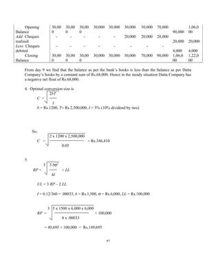
![Return (Rs) Probability
(14 x 55) + (6 x 75) = 1,220 0.3
(14 x 50) + (6 x 65) = 1,090 0.3
(14 x 60) + (6 x 50) = 1,140 0.2
(14 x 70) + (6 x 40) = 1,220 0.2
Expected return = (1,220 x 0.3) + (1,090 x 0.3) + (1,140 x 0.2) + (1,220 x 0.2)
= Rs.1,165
Standard deviation = [(1,220 – 1,165)2
x 0.3 + (1,090 – 1,165)2
x 0.3 +
(1,140 – 1,165)2
x 0.2 + (1,220 – 1,165)2
x 0.2]1/2
= Rs.57.66
The expected return to standard deviation of various options are as follows :
Option
Expected return
(Rs)
Standard deviation
(Rs)
Expected / Standard
return deviation
a 1,150 143 8.04
b 1,200 265 4.53
c 1,175 84 13.99
d 1,165 58 20.09
Option `d’ is the most preferred option because it has the highest return to risk ratio.
3. Expected rates of returns on equity stock A, B, C and D can be computed as follows:
A: 0.10 + 0.12 + (-0.08) + 0.15 + (-0.02) + 0.20 = 0.0783 = 7.83%
6
B: 0.08 + 0.04 + 0.15 +.12 + 0.10 + 0.06 = 0.0917 = 9.17%
6
C: 0.07 + 0.08 + 0.12 + 0.09 + 0.06 + 0.12 = 0.0900 = 9.00%
6
D: 0.09 + 0.09 + 0.11 + 0.04 + 0.08 + 0.16 = 0.095 = 9.50%
6
(a) Return on portfolio consisting of stock A = 7.83%
(b) Return on portfolio consisting of stock A and B in equal
proportions = 0.5 (0.0783) + 0.5 (0.0917)
= 0.085 = 8.5%
19](https://image.slidesharecdn.com/199776069-prasanna-chandra-financial-management-220826060839-ab52aacb/85/199776069-prasanna-chandra-financial-management-pdf-19-320.jpg)
![+ 40000 x PVIF (15,4)
+ 30000 x PVIF (15,5)
= 122646 (A)
Investment = 100,000 (B)
Benefit cost ratio = 1.23 [= (A) / (B)]
8. The NPV’s of the three projects are as follows:
Project
P Q R
Discount rate
0% 400 500 600
5% 223 251 312
10% 69 40 70
15% - 66 - 142 - 135
25% - 291 - 435 - 461
30% - 386 - 555 - 591
9. NPV profiles for Projects P and Q for selected discount rates are as follows:
(a)
Project
P Q
Discount rate (%)
0 2950 500
5 1876 208
10 1075 - 28
15 471 - 222
20 11 - 382
b) (i) The IRR (r ) of project P can be obtained by solving the following
equation for `r’.
-1000 -1200 x PVIF (r,1) – 600 x PVIF (r,2) – 250 x PVIF (r,3)
+ 2000 x PVIF (r,4) + 4000 x PVIF (r,5) = 0
Through a process of trial and error we find that r = 20.13%
(ii) The IRR (r') of project Q can be obtained by solving the following equation for r'
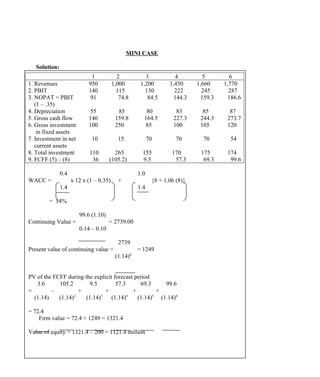
32](https://image.slidesharecdn.com/199776069-prasanna-chandra-financial-management-220826060839-ab52aacb/85/199776069-prasanna-chandra-financial-management-pdf-32-320.jpg)
![MIRR = 11.62%
10
(a) Project A
NPV at a cost of capital of 12%
= - 100 + 25 x PVIFA (12,6)
= Rs.2.79 million
IRR (r ) can be obtained by solving the following equation for r.
25 x PVIFA (r,6) = 100
i.e., r = 12,98%
Project B
NPV at a cost of capital of 12%
= - 50 + 13 x PVIFA (12,6)
= Rs.3.45 million
IRR (r') can be obtained by solving the equation
13 x PVIFA (r',6) = 50
i.e., r' = 14.40% [determined through a process of trial and error]
(b) Difference in capital outlays between projects A and B is Rs.50 million
Difference in net annual cash flow between projects A and B is Rs.12 million.
NPV of the differential project at 12%
= -50 + 12 x PVIFA (12,6)
= Rs.3.15 million
IRR (r'') of the differential project can be obtained from the equation
12 x PVIFA (r'', 6) = 50
i.e., r'' = 11.53%
11
(a) Project M
The pay back period of the project lies between 2 and 3 years. Interpolating in
this range we get an approximate pay back period of 2.63 years/
Project N
The pay back period lies between 1 and 2 years. Interpolating in this range we
get an approximate pay back period of 1.55 years.
34](https://image.slidesharecdn.com/199776069-prasanna-chandra-financial-management-220826060839-ab52aacb/85/199776069-prasanna-chandra-financial-management-pdf-34-320.jpg)
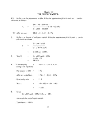
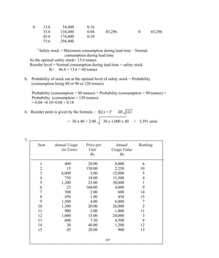
![(c) Accounting break even point (under ‘expected’ scenario)
Fixed costs + depreciation = Rs. 45 million
Contribution margin ratio = 60 / 200 = 0.3
Break even level of sales = 45 / 0.3 = Rs.150 million
Financial break even point (under ‘xpected’ scenario)
i. Annual net cash flow = 0.7143 [ 0.3 x sales – 45 ] + 25
= 0.2143 sales – 7.14
ii. PV (net cash flows) = [0.2143 sales – 7.14 ] x PVIFA (13,10)
= 1.1628 sales – 38.74
iii. Initial investment = 200
iv. Financial break even level
of sales = 238.74 / 1.1628 = Rs.205.31 million
2.
(a) Sensitivity of NPV with respect to quantity manufactured and sold:
(in Rs)
Pessimistic Expected Optimistic
Initial investment 30000 30000 30000
Sale revenue 24000 42000 54000
Variable costs 16000 28000 36000
Fixed costs 3000 3000 3000
Depreciation 2000 2000 2000
Profit before tax 3000 9000 13000
Tax 1500 4500 6500
Profit after tax 1500 4500 6500
Net cash flow 3500 6500 8500
NPV at a cost of
capital of 10% p.a
and useful life of
5 years -16732 - 5360 2222
(b) Sensitivity of NPV with respect to variations in unit price.
Pessimistic Expected Optimistic
Initial investment 30000 30000 30000
Sale revenue 28000 42000 70000
44](https://image.slidesharecdn.com/199776069-prasanna-chandra-financial-management-220826060839-ab52aacb/85/199776069-prasanna-chandra-financial-management-pdf-44-320.jpg)
![= 5.8
A3 = 3 x 0.3 + 4 x 0.5 + 5 x 0.2
= 3.9
NPV = 4.7 / 1.1 +5.8 / (1.1)2
+ 3.9 / (1.1)3
– 10
= Rs.2.00 million
σ1
2
= 0.41
σ2
2
= 0.56
σ3
2
= 0.49
σ1
2
σ2
2
σ3
2
σ2
NPV = + +
(1.1)2
(1.1)4
(1.1)6
= 1.00
σ (NPV) = Rs.1.00 million
4. Expected NPV
4 At
= ∑ - 25,000
t=1 (1.08)t
= 12,000/(1.08) + 10,000 / (1.08)2
+ 9,000 / (1.08)3
+ 8,000 / (1.08)4
– 25,000
= [ 12,000 x .926 + 10,000 x .857 + 9,000 x .794 + 8,000 x .735]
- 25,000
= 7,708
Standard deviation of NPV
4 σt
∑
t=1 (1.08)t
= 5,000 / (1.08) + 6,000 / (1.08)2
+ 5,000 / (1,08)3
+ 6,000 / (1.08)4
= 5,000 x .926 + 6,000 x .857 + 5000 x .794 + 6,000 x .735
= 18,152
5. Expected NPV
46](https://image.slidesharecdn.com/199776069-prasanna-chandra-financial-management-220826060839-ab52aacb/85/199776069-prasanna-chandra-financial-management-pdf-46-320.jpg)
![4 At
= ∑ - 10,000 …. (1)
t=1 (1.06)t
A1 = 2,000 x 0.2 + 3,000 x 0.5 + 4,000 x 0.3
= 3,100
A2 = 3,000 x 0.4 + 4,000 x 0.3 + 5,000 x 0.3
= 3,900
A3 = 4,000 x 0.3 + 5,000 x 0.5 + 6,000 x 0.2
= 4,900
A4 = 2,000 x 0.2 + 3,000 x 0.4 + 4,000 x 0.4
= 3,200
Substituting these values in (1) we get
Expected NPV = NPV
= 3,100 / (1.06)+ 3,900 / 1.06)2
+ 4,900 / (1.06)3
+ 3,200 / (1,06)4
- 10,000 = Rs.3,044
The variance of NPV is given by the expression
4 σ2
t
σ2
(NPV) = ∑ …….. (2)
t=1 (1.06)2t
σ1
2
= [(2,000 – 3,100)2
x 0.2 + (3,000 – 3,100)2
x 0.5
+ (4,000 – 3,100)2
x 0.3]
= 490,000
σ2
2
= [(3,000 – 3,900)2
x 0.4 + (4,000 – 3,900)2
x 0.3
+ (5,000 – 3900)2
x 0.3]
= 690,000
σ3
2
= [(4,000 – 4,900)2
x 0.3 + (5,000 – 4,900)2
x 0.5
+ (6,000 – 4,900)2
x 0.2]
= 490,000
σ4
2
= [(2,000 – 3,200)2
x 0.2 + (3,000 – 3,200)2
x 0.4
+ (4,000 – 3200)2
x 0.4]
= 560,000
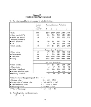
47](https://image.slidesharecdn.com/199776069-prasanna-chandra-financial-management-220826060839-ab52aacb/85/199776069-prasanna-chandra-financial-management-pdf-47-320.jpg)
![Substituting these values in (2) we get
490,000 / (1.06)2
+ 690,000 / (1.06)4
+ 490,000 / (1.06)6
+ 560,000 / (1.08)8
[ 490,000 x 0.890 + 690,000 x 0.792
+ 490,000 x 0.705 + 560,000 x 0.627 ]
= 1,679,150
σ NPV= 1,679,150 = Rs.1,296
NPV – NPV 0 - NPV
Prob (NPV < 0) = Prob. <
σ NPV σ NPV
0 – 3044
= Prob Z <
1296
= Prob (Z < -2.35)
The required probability is given by the shaded area in the following normal curve.
P (Z < - 2.35) = 0.5 – P (-2.35 < Z < 0)
= 0.5 – P (0 < Z < 2.35)
= 0.5 – 0.4906
= 0.0094
So the probability of NPV being negative is 0.0094
Prob (P1 > 1.2) Prob (PV / I > 1.2)
Prob (NPV / I > 0.2)
Prob. (NPV > 0.2 x 10,000)
Prob (NPV > 2,000)
Prob (NPV >2,000)= Prob (Z > 2,000- 3,044 / 1,296)
Prob (Z > - 0.81)
The required probability is given by the shaded area of the following normal
curve:
P(Z > - 0.81) = 0.5 + P(-0.81 < Z < 0)
= 0.5 + P(0 < Z < 0.81)
= 0.5 + 0.2910
= 0.7910
So the probability of P1 > 1.2 as 0.7910
48](https://image.slidesharecdn.com/199776069-prasanna-chandra-financial-management-220826060839-ab52aacb/85/199776069-prasanna-chandra-financial-management-pdf-48-320.jpg)
![6. Given values of variables other than Q, P and V, the net present value model of Bidhan
Corporation can be expressed as:
[Q(P – V) – 3,000 – 2,000] (0.5)+ 2,000 0
5
NPV ∑ + - 30,000
t =1 (1.1)t
(1.1)5
0.5 Q (P – V) – 500
5
∑ = ------------------------------------ - 30,000
t=1 (1.1)t
= [ 0.5Q (P – V) – 500] x PVIFA (10,5) – 30,000
= [0.5Q (P – V) – 500] x 3.791 – 30,000
= 1.8955Q (P – V) – 31,895.5
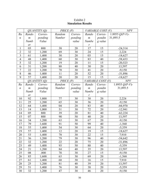
Exhibit 1 presents the correspondence between the values of exogenous variables and the two
digit random number. Exhibit 2 shows the results of the simulation.
Exhibit 1
Correspondence between values of exogenous variables and
two digit random numbers
QUANTITY PRICE VARIABLE COST
Valu
e
Pro
b
Cumulati
ve Prob.
Two digit
random
numbers Valu
e
Pro
b
Cumulati
ve Prob.
Two digit
random
numbers Value Pro
b
Cum
u-
lative
Prob.
Two digit
random
numbers
800 0.1
0
0.10 00 to 09 20 0.4
0
0.40 00 to 39 15 0.3
0
0.30 00 to 29
1,00
0
0.1
0
0.20 10 to 19 30 0.4
0
0.80 40 to 79 20 0.5
0
0.80 30 to 79
1,20
0
0.2
0
0.40 20 to 39 40 0.1
0
0.90 80 to 89 40 0.2
0
1.00 80 to 99
1,40
0
0.3
0
0.70 40 to 69 50 0.1
0
1.00 90 to 99
1,60
0
0.2
0
0.90 70 to 89
1,80
0
0.1
0
1.00 90 to 99
49](https://image.slidesharecdn.com/199776069-prasanna-chandra-financial-management-220826060839-ab52aacb/85/199776069-prasanna-chandra-financial-management-pdf-49-320.jpg)
![31 52 1,400 61 30 58 20 -5,359
32 76 1,600 18 20 41 20 -31,896
33 43 1,400 04 20 49 20 -31,896
34 70 1,600 11 20 59 20 -31,896
35 67 1,400 35 20 26 15 -18,627
36 26 1,200 63 30 22 15 2,224
QUANTITY (Q) PRICE (P) VARIABLE COST (V) NPV
Ru
n
Random
Number
Corre
s-
pondi
ng
Value
Random
Number
Corres-
ponding
value
Rando
m
Numbe
r
Corres-
pondin
g value
1.8955 Q(P-V)-
31,895.5
37 89 1,600 86 40 59 20 28,761
38 94 1,800 00 20 25 15 -14,836
39 09 .800 15 20 29 15 -24,314
40 44 1,400 84 40 21 15 34,447
41 98 1,800 23 20 79 20 -31,896
42 10 1,000 53 30 77 20 -12,941
43 38 1,200 44 30 31 20 -9,150
44 83 1,600 30 20 10 15 -16,732
45 54 1,400 71 30 52 20 -5,359
46 16 1,000 70 30 19 15 -3,463
47 20 1,200 65 30 87 40 -54,642
48 61 1,400 61 30 70 20 -5,359
49 82 1,600 48 30 97 40 -62,224
50 90 1,800 50 30 43 20 2,224
Expected NPV = NPV
50
= 1/ 50 ∑ NPVi
i=1
= 1/50 (-7,20,961)
= 14,419
50
Variance of NPV = 1/50 ∑ (NPVi – NPV)2
i=1
= 1/50 [27,474.047 x 106
]
= 549.481 x 10⁶
51](https://image.slidesharecdn.com/199776069-prasanna-chandra-financial-management-220826060839-ab52aacb/85/199776069-prasanna-chandra-financial-management-pdf-51-320.jpg)
![Standard deviation of NPV = 549.481 x 106
= 23,441
7. To carry out a sensitivity analysis, we have to define the range and the most likely values of
the variables in the NPV Model. These values are defined below
Variable Range Most likely value
I Rs.30,000 – Rs.30,000 Rs.30,000
k 10% - 10% 10%
F Rs.3,000 – Rs.3,000 Rs.3,000
D Rs.2,000 – Rs.2,000 Rs.2,000
T 0.5 – 0.5 0.5
N 5 – 5 5
S 0 – 0 0
Q Can assume any one of the values - 1,400*
800, 1,000, 1,200, 1,400, 1,600 and 1,800
P Can assume any of the values 20, 30, 30**
40 and 50
V Can assume any one of the values 20*
15,20 and 40
----------------------------------------------------------------------------------------
* The most likely values in the case of Q, P and V are the values that have the
highest probability associated with them
** In the case of price, 20 and 30 have the same probability of occurrence viz 0.4. We
have chosen 30 as the most likely value because the expected value of the
distribution is closer to 30
Sensitivity Analysis with Reference to Q
The relationship between Q and NPV given the most likely values of other
variables is given by
5 [Q (30-20) – 3,000 – 2,000] x 0.5 + 2,000 0
NPV = ∑ + - 30,000
t=1 (1.1)t
(1.1)5
5 5Q - 500
= ∑ - 30,000
t=1 (1.1)t
The net present values for various values of Q are given in the following table:
52](https://image.slidesharecdn.com/199776069-prasanna-chandra-financial-management-220826060839-ab52aacb/85/199776069-prasanna-chandra-financial-management-pdf-52-320.jpg)
![Q 800 1,000 1,200 1,400 1,600 1,800
NPV -16,732 -12,941 -9,150 -5,359 -1,568 2,224
Sensitivity analysis with reference to P
The relationship between P and NPV, given the most likely values of other variables is defined as
follows:
5 [1,400 (P-20) – 3,000 – 2,000] x 0.5 + 2,000 0
NPV = ∑ + - 30,0
t=1 (1.1)t
(1.1)5
5 700 P – 14,500
= ∑ - 30,000
t=1 (1.1)t
The net present values for various values of P are given below :
P (Rs) 20 30 - 40 50
NPV(Rs) -31,896 -5,359 21,179 47,716
8. NPV - 5 0 5 10 15 20
(Rs.in lakhs)
PI 0.9 1.00 1.10 1.20 1.30 1.40
Prob. 0.02 0.03 0.10 0.40 0.30 0.15
6
Expected PI = PI = ∑ (PI)j Pj
j=1
= 1.24
6
Standard deviation of P1 = ∑ (PIj - PI) 2
Pj
j=1
= √ .01156
= .1075
The standard deviation of P1 is .1075 for the given investment with an expected PI of 1.24.
The maximum standard deviation of PI acceptable to the company for an investment with an
expected PI of 1.25 is 0.30.
53](https://image.slidesharecdn.com/199776069-prasanna-chandra-financial-management-220826060839-ab52aacb/85/199776069-prasanna-chandra-financial-management-pdf-53-320.jpg)
![6,580 7,040 7,380 7,600 5,600
+ + + +
(1.08) (1.08)2
(1.08)3
(1.08)4
(1.08)5
= 27,386
Net present value of the Project = (27,386 – 30,000
= Rs. –2,614
MINICASE
Solution:
1. The expected NPV of the turboprop aircraft
0.65 (5500) + 0.35 (500)
NPV = - 11000 +
(1.12)
0.65 [0.8 (17500) + 0.2 (3000)] + 0.35 [0.4 (17500) + 0.6 (3000)]
+
(1.12)2
= 2369
2. If Southern Airways buys the piston engine aircraft and the demand in year 1 turns out to be
high, a further decision has to be made with respect to capacity expansion. To evaluate the
piston engine aircraft, proceed as follows:
First, calculate the NPV of the two options viz., ‘expand’ and ‘do not expand’ at decision
point D2:
0.8 (15000) + 0.2 (1600)
Expand : NPV = - 4400 +
1.12
= 6600
0.8 (6500) + 0.2 (2400)
Do not expand : NPV =
1.12
= 5071
55](https://image.slidesharecdn.com/199776069-prasanna-chandra-financial-management-220826060839-ab52aacb/85/199776069-prasanna-chandra-financial-management-pdf-55-320.jpg)
![Second, truncate the ‘do not expand’ option as it is inferior to the ‘expand’ option. This
means that the NPV at decision point D2 will be 6600
Third, calculate the NPV of the piston engine aircraft option.
0.65 (2500+6600) + 0.35 (800)
NPV = – 5500 +
1.12
0.35 [0.2 (6500) + 0.8 (2400)]
+
(1.12)2
= – 5500 + 5531 + 898 = 929
3. The value of the option to expand in the case of piston engine aircraft
If Southern Airways does not have the option of expanding capacity at the end of year 1, the
NPV of the piston engine aircraft would be:
0.65 (2500) + 0.35 (800)
NPV = – 5500 +
1.12
0.65 [0.8 (6500) + 0.2 (2400)] + 0.35 [0.2 (6500) + 0.8 (2400)]
+
(1.12)2
= - 5500 + 1701 + 3842 = 43
Thus the option to expand has a value of 929 – 43 = 886
4. Value of the option to abandon if the turboprop aircraft can be sold for 8000 at the end of year
1
If the demand in year 1 turns out to be low, the payoffs for the ‘continuation’ and
‘abandonment’ options as of year 1 are as follows.
0.4 (17500) + 0.6 (3000)
Continuation: = 7857
1.12
56](https://image.slidesharecdn.com/199776069-prasanna-chandra-financial-management-220826060839-ab52aacb/85/199776069-prasanna-chandra-financial-management-pdf-56-320.jpg)
![Abandonment : 8000
Thus it makes sense to sell off the aircraft after year 1, if the demand in year 1 turns out to be
low.
The NPV of the turboprop aircraft with abandonment possibility is
0.65 [5500 +{0.8 (17500) + 0.2 (3000)}/ (1.12)] + 0.35 (500 +8000)
NPV = - 11,000 +
(1.12)
12048 + 2975
= - 11,000 + = 2413
1.12
Since the turboprop aircraft without the abandonment option has a value of 2369, the
value of the abandonment option is : 2413 – 2369 = 44
5. The value of the option to abandon if the piston engine aircraft can be sold for 4400 at the
end of year 1:
If the demand in year 1 turns out to be low, the payoffs for the ‘continuation’ and
‘abandonment’ options as of year 1 are as follows:
0.2 (6500) + 0.8 (2400)
Continuation : = 2875
1.12
Abandonment : 4400
Thus, it makes sense to sell off the aircraft after year 1, if the demand in year 1 turns out to
be low.
The NPV of the piston engine aircraft with abandonment possibility is:
0.65 [2500 + 6600] + 0.35 [800 + 4400]
NPV = - 5500 +
1.12
5915 + 1820
= - 5500 + = 1406
1.12
For the piston engine aircraft the possibility of abandonment increases the NPV
57](https://image.slidesharecdn.com/199776069-prasanna-chandra-financial-management-220826060839-ab52aacb/85/199776069-prasanna-chandra-financial-management-pdf-57-320.jpg)

![= 7.35 + 0.75 + 2.22
= 10.32%
g. Cost of capital for the new business
0.5 [7 + 1.5 (7)] + 0.5 [ 11 (1 – 0.3)]
8.75 + 3.85
= 12.60%
64](https://image.slidesharecdn.com/199776069-prasanna-chandra-financial-management-220826060839-ab52aacb/85/199776069-prasanna-chandra-financial-management-pdf-64-320.jpg)
![Chapter 15
CAPITAL BUDGETING : EXTENSIONS
1. EAC
(Plastic Emulsion) = 300000 / PVIFA (12,7)
= 300000 / 4.564
= Rs.65732
EAC
(Distemper Painting) = 180000 / PVIFA (12,3)
= 180000 / 2.402
= Rs.74938
Since EAC of plastic emulsion is less than that of distemper painting, it is the preferred
alternative.
2. PV of the net costs associated with the internal transportation system
= 1 500 000 + 300 000 x PVIF (13,1) + 360 000 x PVIF (13,2)
+ 400 000 x PVIF (13,3) + 450 000 x PVIF (13,4)
+ 500 000 x PVIF (13,5) - 300 000 x PVIF (13,5)
= 2709185
EAC of the internal transportation system
= 2709185 / PVIFA (13,5)
= 2709185 / 3.517
= Rs.770 311
3. EAC [ Standard overhaul]
= 500 000 / PVIFA (14,6)
= 500 000 / 3.889
= Rs.128568 ……… (A)
EAC [Less costly overhaul]
= 200 000 / PVIFA (14,2)
= 200 000 / 1.647
= Rs.121433 ……… (B)
Since (B) < (A), the less costly overhaul is preferred alternative.
65](https://image.slidesharecdn.com/199776069-prasanna-chandra-financial-management-220826060839-ab52aacb/85/199776069-prasanna-chandra-financial-management-pdf-65-320.jpg)
![4.
(a) Base case NPV
= -12,000,000 + 3,000,000 x PVIFA (20,6)
= -12,000,000 + 997,8000
= (-) Rs.2,022,000
(b) Issue costs = 6,000,000 / 0.88 - 6,000,000
= Rs.818 182
Adjusted NPV after adjusting for issue costs
= - 2,022,000 – 818,182
= - Rs.2,840,182
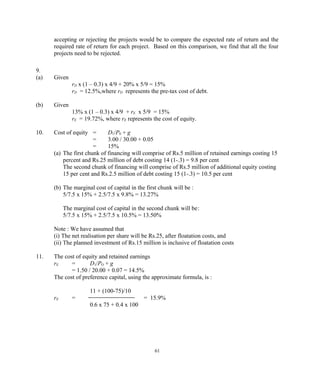
(c) The present value of interest tax shield is calculated below :
Year Debt outstanding at Interest Tax shield Present value of
the beginning tax shield
1 6,000,000 1,080,000 324,000 274,590
2 6,000,000 1,080,000 324,000 232,697
3 5,250,000 945,000 283,000 172,538
4 4,500,000 810,000 243,000 125,339
5 3,750,000 675,000 202,000 88,513
6 3,000,000 540,000 162,000 60,005
7 2,225,000 400,500 120,000 37,715
8 1,500,000 270,000 81,000 21,546
9 750,000 135,000 40,500 9,133
Present value of tax shield = Rs.1,022,076
5.
(a) Base case BPV
= - 8,000,000 + 2,000,000 x PVIFA (18,6)
= - Rs.1,004,000
(b) Adjusted NPV after adjustment for issue cost of external equity
= Base case NPV – Issue cost
= - 1,004,000 – [ 3,000,000 / 0.9 – 3,000,000]
= - Rs.1,337,333
66](https://image.slidesharecdn.com/199776069-prasanna-chandra-financial-management-220826060839-ab52aacb/85/199776069-prasanna-chandra-financial-management-pdf-66-320.jpg)
![1,800,000
(EBIT – 1,500,000) (1 – 0.6)
EPSB =
1,000,000
Equating EPSA and EPSB , we get
(EBIT – 0 ) (1 – 0.6) (EBIT – 1,500,000) (1 – 0.6)
=
1,800,000 1,000,000
Solving this we get EBIT = 3,375,000 or 3.375 million
Thus the debt alternative is better than the equity alternative when
EBIT > 3.375 million
EBIT – EBIT 3.375 – 7.000
Prob(EBIT>3,375,000) = Prob >
σ EBIT 3.000
= Prob [z > - 1.21]
= 0.8869
4. ROE = [ ROI + ( ROI – r ) D/E ] (1 – t )
15 = [ 14 + ( 14 – 8 ) D/E ] ( 1- 0.5 )
D/E = 2.67
5. ROE = [12 + (12 – 9 ) 0.6 ] (1 – 0.6)
= 5.52 per cent
6. 18 = [ ROI + ( ROI – 8 ) 0.7 ] ( 1 – 0.5)
ROI = 24.47 per cent
EBIT
7. a. Interest coverage ratio =
Interest on debt
150
=
40
= 3.75
EBIT + Depreciation
b. Cash flow coverage ratio =
Loan repayment instalment
75](https://image.slidesharecdn.com/199776069-prasanna-chandra-financial-management-220826060839-ab52aacb/85/199776069-prasanna-chandra-financial-management-pdf-75-320.jpg)
![Chapter 23
Debt Analysis and Management
1. (i) Initial Outlay
(a) Cost of calling the old bonds
Face value of the old bonds 250,000,000
Call premium 15,000,000
265,000,000
(b) Net proceeds of the new bonds
Gross proceeds 250,000,000
Issue costs 10,000,000
240,000,000
(c) Tax savings on tax-deductible expenses
Tax rate[Call premium+Unamortised issue cost on
the old bonds] 9,200,000
0.4 [ 15,000,000 + 8,000,000]
Initial outlay i(a) – i(b) – i(c) 15,800,000
(ii) Annual Net Cash Savings
(a) Annual net cash outflow on old bonds
Interest expense 42,500,000
- Tax savings on interest expense and amortisation of
issue expenses 17,400,000
0.4 [42,500,000 + 8,000,000/10]
25,100,000
(b) Annual net cash outflow on new bonds
Interest expense 37,500,000
- Tax savings on interest expense and amortisation of
issue cost 15,500,000
0.4 [ 37,500,000 – 10,000,000/8]
22,000,000
Annual net cash savings : ii(a) – ii(b) 3,100,000
82](https://image.slidesharecdn.com/199776069-prasanna-chandra-financial-management-220826060839-ab52aacb/85/199776069-prasanna-chandra-financial-management-pdf-82-320.jpg)
![(iii) Present Value of the Annual Cash Savings
Present value of an 8-year annuity of 3,100,000 at a
discount rate of 9 per cent which is the post –tax cost
of new bonds 3,100,000 x 5.535 17,158,500
(iv) Net Present Value of Refunding the Bonds
(a) Present value of annual cash savings 17,158,500
(b) Net initial outlay 15,800,000
(c) Net present value of refunding the bonds :
iv(a) – iv(b). 1,358,500
2. (i) Initial Outlay
(a) Cost of calling the old bonds
Face value of the old bonds 120,000,000
Call premium 4,800,000
124,800,000
(b) Net proceeds of the new issue
Gross proceeds 120,000,000
Issue costs 2,400,000
117,600,000
(c) Tax savings on tax-deductible expenses 3,120,000
Tax rate[Call premium+Unamortised issue costs on
the old bond issue]
0.4 [ 4,800,000 + 3,000,000]
Initial outlay i(a) – i(b) – i(c) 4,080,000
(ii) Annual Net Cash Savings
(a) Annual net cash out flow on old bonds
Interest expense 19,200,000
- Tax savings on interest expense and amortisation of
issue costs 7,920,000
0.4[19,200,000 + 3,000,000/5]
11,280,000
(b) Annual net cash outflow on new bonds
Interest expense 18,000,000
- Tax savings on interest expense and amortistion of issue
costs 7,392,000
0.4[18,000,000 + 2,400,000/5]
10,608,000
Annual net cash savings : ii(a) – ii(b) 672,000
(iii) Present Value of the Annual Net Cash Savings
83](https://image.slidesharecdn.com/199776069-prasanna-chandra-financial-management-220826060839-ab52aacb/85/199776069-prasanna-chandra-financial-management-pdf-83-320.jpg)
- k ΔI
Δ S
Δ I = x ACP x V
360
Δ S = Rs.10 million, V=0.85, bn =0.08, ACP= 60 days, k=0.15, t = 0.40
Hence, ΔRI = [ 10,000,000(1-0.85)- 10,000,000 x 0.08 ] (1-0.4)
-0.15 x 10,000,000 x 60 x 0.85
360
= Rs. 207,500
2. Δ RI = [ΔS(1-V)- ΔSbn] (1-t) – k Δ I
So ΔS
Δ I = (ACPN – ACPo) +V(ACPN)
360 360
98](https://image.slidesharecdn.com/199776069-prasanna-chandra-financial-management-220826060839-ab52aacb/85/199776069-prasanna-chandra-financial-management-pdf-98-320.jpg)
![ΔS=Rs.1.5 million, V=0.80, bn=0.05, t=0.45, k=0.15, ACPN=60, ACPo=45, So=Rs.15 million
Hence ΔRI = [1,500,000(1-0.8) – 1,500,000 x 0.05] (1-.45)
-0.15 (60-45) 15,000,000 + 0.8 x 60 x 1,500,000
360 360
= 123750 – 123750 = Rs. 0
3. Δ RI = [ΔS(1-V) –Δ DIS ] (1-t) + k Δ I
Δ DIS = pn(So+ΔS)dn – poSodo
So ΔS
Δ I = (ACPo-ACPN) - x ACPN x V
360 360
So =Rs.12 million, ACPo=24, V=0.80, t= 0.50, r=0.15, po=0.3, pn=0.7,
ACPN=16, ΔS=Rs.1.2 million, do=.01, dn= .02
Hence
ΔRI = [ 1,200,000(1-0.80)-{0.7(12,000,000+1,200,000).02-
0.3(12,000,000).01}](1-0.5)
12,000,000 1,200,000
+ 0.15 (24-16) - x 16 x 0.80
360 360
= Rs.79,200
4. Δ RI = [ΔS(1-V)- ΔBD](1-t) –kΔ I
ΔBD=bn(So+ΔS) –boSo
So ΔS
ΔI = (ACPN –ACPo) + x ACPN x V
360 360
So=Rs.50 million, ACPo=25, V=0.75, k=0.15, bo=0.04, ΔS=Rs.6 million,
ACPN=40 , bn= 0.06 , t = 0.3
ΔRI = [ Rs.6,000,000(1-.75) –{.06(Rs.56,000,000)-.04(Rs.50,000,000)](1-0.3)
99](https://image.slidesharecdn.com/199776069-prasanna-chandra-financial-management-220826060839-ab52aacb/85/199776069-prasanna-chandra-financial-management-pdf-99-320.jpg)
 – kΔI
So=Rs.50 million, ΔS=Rs.10 million, do=0.02, po=0.70, dn=0.03,pn=0.60,
ACPo=20 days, ACPN=24 days, V=0.85, k=0.12 , and t = 0.40
ΔDIS = 0.60 x 60 x 0.03 – 0.70 x 50 x 0.2
= Rs.0.38 million
50 10
Δ I = (24-20) + x 24 x 0.85
360 360
= Rs.1.2222 million
Δ RI = [ 10,000,000 (1-.85) – 380,000 ] (1-.4) – 0.12 x 1,222,222
100](https://image.slidesharecdn.com/199776069-prasanna-chandra-financial-management-220826060839-ab52aacb/85/199776069-prasanna-chandra-financial-management-pdf-100-320.jpg)
![• Post-tax cost of capital : 12 percent
• ACP on credit sales : 20 days
Effect of Relaxing the Credit Standards on Residual Income
Incremental sales : Rs.50 million
Bad debt losses on incremental sales: 12 percent
ACP remains unchanged at 20 days
∆RI = [∆S(1 – V) - ∆Sbn] (1 – t) – R ∆ I
∆S
where ∆ I = x ACP x V
360
∆ RI = [50,000,000 (1-0.8) – 50,000,000 x 0.12] (1 – 0.3)
50,000,000
- 0.12 x x 20 x 0.8
360
= 2,800,000 – 266,667 = 2,533,333
Effect of Extending the Credit Period on Residual Income
∆ RI = [∆S(1 – V) - ∆Sbn] (1 – t) – R ∆ I
So ∆S
where ∆I = (ACPn – ACPo) + V (ACPn)
360 360
∆RI = [50,000,000 (1 – 0.8) – 50,000,000 x 0] (1 – 0.3)
800,000,000 50,000,000
- 0.12 (50 – 20) x + 0.8 x 50 x
360 360
= 7,000,000 – 8,666,667
= - Rs.1,666,667
Effect of Relaxing the Cash Discount Policy on Residual Income
∆RI = [∆S (1 – V) - ∆ DIS] (1 – t) + R ∆ I
102](https://image.slidesharecdn.com/199776069-prasanna-chandra-financial-management-220826060839-ab52aacb/85/199776069-prasanna-chandra-financial-management-pdf-102-320.jpg)
![where ∆ I = savings in receivables investment
So ∆S
= (ACPo – ACPn) – V x ACPn
360 360
800,000,000 20,000,000
= (20 – 16) – 0.8 x x 16
360 360
= 8,888,889 – 711,111 = 8,177,778
∆ DIS = increase in discount cost
= pn (So + ∆S) dn – po So do
= 0.7 (800,000,000 + 20,000,000) x 0.02 – 0.5 x 800,000,000 x 0.01
= 11,480,000 – 4,000,000 = 7,480,000
So, ∆RI = [20,000,000 (1 – 0.8) – 7,480,000] (1 – 0.3) + 0.12 x 8,177,778
= - 2,436,000 + 981,333
= - 1,454,667
Chapter 29
INVENTORY MANAGEMENT
1.
a. No. of Order Ordering Cost Carrying Cost Total Cost
Orders Per Quantity (U/Q x F) Q/2xPxC of Ordering
Year (Q) (where and Carrying
(U/Q) PxC=Rs.30)
Units Rs. Rs. Rs.
1 250 200 3,750 3,950
2 125 400 1,875 2,275
5 50 1,000 750 1,750
10 25 2,000 375 2,375
2 UF 2x250x200
103](https://image.slidesharecdn.com/199776069-prasanna-chandra-financial-management-220826060839-ab52aacb/85/199776069-prasanna-chandra-financial-management-pdf-103-320.jpg)
![b. Economic Order Quantity (EOQ) = =
PC 30
2UF = 58 units (approx)
2. a EOQ =
PC
U=10,000 , F=Rs.300, PC= Rs.25 x 0.25 =Rs.6.25
2 x 10,000 x 300
EOQ = = 980
6.25
10000
b. Number of orders that will be placed is = 10.20
980
Note that though fractional orders cannot be placed, the number of orders
relevant for the year will be 10.2 . In practice 11 orders will be placed during the year. However,
the 11th
order will serve partly(to the extent of 20 percent) the present year and partly(to the
extent of 80 per cent) the following year. So only 20 per cent of the ordering cost of the 11th
order relates to the present year. Hence the ordering cost for the present year will be 10.2 x
Rs.300
c. Total cost of carrying and ordering inventories
980
= [ 10.2 x 300 + x 6.25 ] = Rs.6122.5
2
3. U=6,000, F=Rs.400 , PC =Rs.100 x 0.2 =Rs.20
2 x 6,000 x 400
EOQ = = 490 units
20
U U Q’(P-D)C Q* PC
Δπ = UD + - F- -
Q* Q’ 2 2
6,000 6,000
= 6000 x .5 + - x 400
490 1,000
1,000 (95)0.2 490 x 100 x 0.2
- -
2 2
104](https://image.slidesharecdn.com/199776069-prasanna-chandra-financial-management-220826060839-ab52aacb/85/199776069-prasanna-chandra-financial-management-pdf-104-320.jpg)
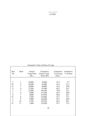
![*
Note that if the DUR is 4 units with a probability of 0.3 and the LT is 5 days with
a probability of 0.6, the requirement for the combination DUR = 4 units and LT =
5 days is 20 units with a probability of 0.3x0.6 = 0.18. We have assumed that the
probability distributions of DUR and LT are independent. All other entries in the
table are derived similarly.
The normal (expected) consumption during the lead time is :
20x0.18 + 30x0.30 + 40x0.12 + 40x0.06 + 60x0.10 + 80x0.04 + 60x0.06 + 90x0.10 +
120x0.04 = 46.4 tonnes
a. Costs associated with various levels of safety stock are given below :
Safety Stock Stock out Probability Expected Carrying Total Cost
Stock* outs(in Cost Stock out Cost
tonnes)
1 2 3 4 5 6 7
[3x4] [(1)x1,000] [5+6]
Tonnes Rs. Rs. Rs.
73.6 0 0 0 0 73,600 73,600
43.6 30 120,000 0.04 4,800 43,600 48,400
33.6 10 40,000 0.10
40 160,000 0.04 10,400 33,600 44,000
13.6 20 80,000 0.04
30 120,000 0.10 24,800 13,600 38,400
60 240,000 0.04
106](https://image.slidesharecdn.com/199776069-prasanna-chandra-financial-management-220826060839-ab52aacb/85/199776069-prasanna-chandra-financial-management-pdf-106-320.jpg)
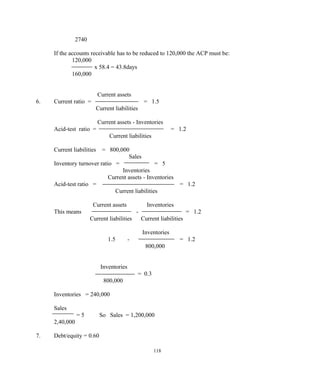
![(a) Key ratios for 20 X 5
12.4
Current ratio = = 0.93
13.4
8.8 + 6.7
Debt-equity ratio = = 0.98
6.5 + 9.3
57.4
Total assets turnover ratio = = 1.96
[(34 – 6.6) + (38 – 6.7)] / 2
3.0
Net profit margin = = 5.2 percent
57.4
5
Earning power = = 17.0 percent
[(34 – 6.6) + (38 – 6.7)] / 2
3.0
Return on equity = = 20.2 percent
(13.9 + 15.8) / 2
(b) Dupont Chart for 20 x 5
–
÷
122
Return on
total assets
10.2%
Net profit
margin
5.2%
Net profit
3.0
Net sales
57.4
Net sales +/-
Non-op. surplus
deficit 57.8
Total costs
54.8](https://image.slidesharecdn.com/199776069-prasanna-chandra-financial-management-220826060839-ab52aacb/85/199776069-prasanna-chandra-financial-management-pdf-122-320.jpg)
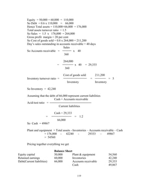
![5. Working capital 400 480 576 691 829 912
6. ∆Working capital 80 96 115 138 83
7. FCFF 11 13 16 19 273
(3-4-6)
Discount factor 0.876 0.767 0.672 .589
Present value 9.64 9.97 10.76 11.19
Cost of capital for the high growth period
0.4 [12% + 1.25 x 7%] + 0.6 [15% (1 - .35)]
8.3% + 5.85%
= 14.15%
Cost of capital for the stable growth period
0.5 [12% + 1.00 x 6%] + 0.5 [14% (1 - .35)]
9% + 4.55%
= 13.55%
Present value of FCFF during the explicit forecast period
= 9.64 + 9.97 + 10.76 + 11.19 = 41.56
273 273
Horizon value = = = 7690
0.1355 – 0.10 0.0355
Present value of horizon value = 4529.5
Value of the firm = 41.56 + 4529.50 = Rs.4571.06 million
3. The WACC for different periods may be calculated :
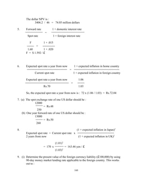
WACC in the high growth period
Year kd(1-t) = 15% (1-t) ke = Rf + β x Market risk premium ka = wd kd (1-t)+ we ke
1 15 (0.94) = 14.1% 12 + 1.3 x 7 = 21.1% 0.5 x 14.1 + 0.5 x 21.1 = 17.6%
2 15 (0.88) = 13.2% 21.1% 0.5 x 13.2 + 0.5 x 21.1 = 17.2%
3 15 (0.82) = 12.3% 21.1% 0.5 x 12.3 + 0.5 x 21.1 = 16.7%
4 15 (0.76) = 11.4% 21.1% 0.5 x 11.4 + 0.5 x 21.1 = 16.3%
5 15 (0.70) = 10.5% 21.1% 0.5 x 10.5 + 0.5 x 21.1 = 15.8%
WACC in the transition period
kd(1-t) = 14 (1 – 0.3) = 9.8%
143](https://image.slidesharecdn.com/199776069-prasanna-chandra-financial-management-220826060839-ab52aacb/85/199776069-prasanna-chandra-financial-management-pdf-143-320.jpg)


![[wacc] weighted average cost of capital](https://cdn.slidesharecdn.com/ss_thumbnails/anuragmathur-210703072911-thumbnail.jpg?width=640&height=640&fit=bounds)


