01-05-2023, SOL_DU_MBAFT_6202_Dijkstra’s Algorithm Dated 1st May 23.pdf

By
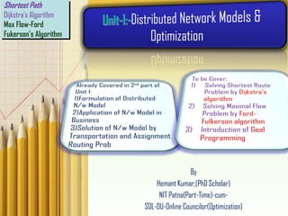
Hemant Kumar,(PhD Scholar)
NIT Patna(Part-Time)-cum-
SOL-DU-Online Councilor(Optimization)
Shortest Path
Dijkstra’s Algorithm
Max Flow-Ford
Fukerson’s Algorithm

• Works when all of the weights are positive.
• Provides the shortest paths from a source to all other vertices in the graph.
– Can be terminated early once the shortest path to t is found if desired.
Shortest Path
– Consider the following graph with positive weights and cycles.

• A first attempt at solving this problem might require an
array of Boolean values, all initially false, that indicate
whether we have found a path from the source.
1 F
2 F
3 F
4 F
5 F
6 F
7 F
8 F
9 F

• Graphically, we will denote this with check
boxes next to each of the vertices (initially
unchecked)

• We will work bottom up.
– Note that if the starting vertex has any adjacent
edges, then there will be one vertex that is the
shortest distance from the starting vertex. This is
the shortest reachable vertex of the graph.
• We will then try to extend any existing paths
to new vertices.
• Initially, we will start with the path of length 0
– this is the trivial path from vertex 1 to itself

• If we now extend this path, we should
consider the paths
– (1, 2) length 4
– (1, 4) length 1
– (1, 5) length 8
The shortest path so far is (1, 4) which is of
length 1.

• Thus, if we now examine vertex 4, we may
deduce that there exist the following paths:
– (1, 4, 5) length 12
– (1, 4, 7) length 10
– (1, 4, 8) length 9

• We need to remember that the length of
that path from node 1 to node 4 is 1
• Thus, we need to store the length of a
path that goes through node 4:
– 5 of length 12
– 7 of length 10
– 8 of length 9

• We have already discovered that there is a
path of length 8 to vertex 5 with the path
(1, 5).
• Thus, we can safely ignore this longer
path.

• We now know that:
– There exist paths from vertex 1 to
vertices {2,4,5,7,8}.
– We know that the shortest path
from vertex 1 to vertex 4 is of
length 1.
– We know that the shortest path to
the other vertices {2,5,7,8} is at
most the length listed in the table
to the right.
Vertex Length
1 0
2 4
4 1
5 8
7 10
8 9

• There cannot exist a shorter path to either of the vertices
1 or 4, since the distances can only increase at each
iteration.
• We consider these vertices to be
visited
Vertex Length
1 0
2 4
4 1
5 8
7 10
8 9
If you only knew this information and
nothing else about the graph, what is the
possible lengths from vertex 1 to vertex 2?
What about to vertex 7?

• In Dijkstra’s algorithm, we always take the next unvisited
vertex which has the current shortest path from the
starting vertex in the table.
• This is vertex 2

• We can try to update the shortest paths to vertices 3 and 6
(both of length 5) however:
– there already exists a path of length 8 < 10 to vertex 5 (10 = 4 +
6)
– we already know the shortest path to 4 is 1

• To keep track of those vertices to which no
path has reached, we can assign those
vertices an initial distance of either
– infinity (∞ ),
– a number larger than any possible path, or
– a negative number
• For demonstration purposes, we will use ∞

• As well as finding the length of the shortest path, we’d like
to find the corresponding shortest path
• Each time we update the shortest distance to a particular
vertex, we will keep track of the predecessor used to reach
this vertex on the shortest path.

• We will store a table of pointers, each
initially 0
• This table will be updated each
time a distance is updated
1 0
2 0
3 0
4 0
5 0
6 0
7 0
8 0
9 0

• Graphically, we will display the reference
to the preceding vertex by a red arrow
– if the distance to a vertex is ∞, there will be no
preceding vertex
– otherwise, there will be exactly one preceding
vertex

• Thus, for our initialization:
– we set the current distance to the initial vertex
as 0
– for all other vertices, we set the current
distance to ∞
– all vertices are initially marked as unvisited
– set the previous pointer for all vertices to null

• Thus, we iterate:
– find an unvisited vertex which has the shortest
distance to it
– mark it as visited
– for each unvisited vertex which is adjacent to
the current vertex:
• add the distance to the current vertex to the weight
of the connecting edge
• if this is less than the current distance to that
vertex, update the distance and set the parent
vertex of the adjacent vertex to be the current
vertex

• Halting condition:
– we successfully halt when the vertex we are
visiting is the target vertex
– if at some point, all remaining unvisited
vertices have distance ∞, then no path from
the starting vertex to the end vertex exits
• Note: We do not halt just because we
have updated the distance to the end
vertex, we have to visit the target vertex.

• Consider the graph:
– the distances are appropriately initialized
– all vertices are marked as being unvisited
Dijkstra’s Algorithm Example

Example
• Visit vertex 1 and update its neighbours,
marking it as visited
– the shortest paths to 2, 4, and 5 are updated

• The next vertex we visit is vertex 4
– vertex 5 1 + 11 ≥ 8 don’t update
– vertex 7 1 + 9 < ∞ update

Example
• Next, visit vertex 2
– vertex 4 already visited

• Next, we have a choice of either 3 or 6
• We will choose to visit 3
– vertex 5 5 + 2 < 8 update

• We then visit 6

• Next, we finally visit vertex 5:
– vertices 4 and 6 have already been visited

• Given a choice between vertices 7 and 8,
we choose vertex 7
– vertices 5 has already been visited

• Next, we visit vertex 8:

• Finally, we visit the end vertex
• Therefore, the shortest path from 1 to 9
has length 11

• We can find the shortest path by working
back from the final vertex:
– 9, 8, 5, 3, 2, 1
• Thus, the shortest path is (1, 2, 3, 5, 8, 9)

• In the example, we visited all vertices in
the graph before we finished
• This is not always the case, consider the
next example

Example
• Find the shortest path from 1 to 4:
– the shortest path is found after only three vertices are
visited
– we terminated the algorithm as soon as we reached
vertex 4
– we only have useful information about 1, 3, 4
– we don’t have the shortest path to vertex 2

d[s]  0
for each v  V – {s}
do d[v]  
S  
Q  V ⊳ Q is a priority queue maintaining V – S
while Q  
do u  EXTRACT-MIN(Q)
S  S  {u}
for each v  Adj[u]
do if d[v] > d[u] + w(u, v)
then d[v]  d[u] + w(u, v)
p[v]  u

d[s]  0
for each v  V – {s}
do d[v]  
S  
Q  V ⊳ Q is a priority queue maintaining V – S
while Q  
do u  EXTRACT-MIN(Q)
S  S  {u}
for each v  Adj[u]
do if d[v] > d[u] + w(u, v)
then d[v]  d[u] + w(u, v)
p[v]  u
relaxation
step
Implicit DECREASE-KEY

A
B D
C E
10
3
1 4 7 9
8
2
2
Graph with
nonnegative
edge weights:

A
B D
C E
10
3
1 4 7 9
8
2
2
Initialize:
A B C D E
Q:
0    
S: {}
0

 


A
B D
C E
10
3
1 4 7 9
8
2
2
A B C D E
Q:
0    
S: { A }
0

 

“A”  EXTRACT-MIN(Q):

A
B D
C E
10
3
1 4 7 9
8
2
2
A B C D E
Q:
0    
S: { A }
0
10
3 

10 3
Relax all edges leaving A:
 

A
B D
C E
10
3
1 4 7 9
8
2
2
A B C D E
Q:
0    
S: { A, C }
0
10
3 

10 3
“C”  EXTRACT-MIN(Q):
 

A
B D
C E
10
3
1 4 7 9
8
2
2
A B C D E
Q:
0    
S: { A, C }
0
7
3 5
11
10 3
7 11 5
Relax all edges leaving C:
 

A
B D
C E
10
3
1 4 7 9
8
2
2
A B C D E
Q:
0    
S: { A, C, E }
0
7
3 5
11
10 3
7 11 5
“E”  EXTRACT-MIN(Q):
 

A
B D
C E
10
3
1 4 7 9
8
2
2
A B C D E
Q:
0    
S: { A, C, E }
0
7
3 5
11
10 3  
7 11 5
7 11
Relax all edges leaving E:

A
B D
C E
10
3
1 4 7 9
8
2
2
A B C D E
Q:
0    
S: { A, C, E, B }
0
7
3 5
11
10 3  
7 11 5
7 11
“B”  EXTRACT-MIN(Q):

A
B D
C E
10
3
1 4 7 9
8
2
2
A B C D E
Q:
0    
S: { A, C, E, B }
0
7
3 5
9
10 3  
7 11 5
7 11
Relax all edges leaving B:
9

A
B D
C E
10
3
1 4 7 9
8
2
2
A B C D E
Q:
0    
S: { A, C, E, B, D }
0
7
3 5
9
10 3  
7 11 5
7 11
9
“D”  EXTRACT-MIN(Q):

• Begins at source and examines the graph to determine the shortest route
between source and every other node of network.
• For given a weighted directed graph, we can find the shortest distance between
two vertices by:
– starting with a trivial path containing the initial vertex
– growing this path by always going to the next vertex which has the shortest
current path
Dijkstra’s Algorithm Summary

t
f
f
-
A
A
A
-
-
f t
t
t
B
B
f t
-
4
2
5
∞
∞
F
f t 10
8
9
Give the shortest path tree for node
A for this graph using Dijkstra’s
shortest path algorithm. Show your
work with the 3 arrays given and
draw the resultant shortest path tree
with edge weights included.
Dijkstra’s Algorithm-For Practice

What is Network Flow
What us Logistics Routing Plans: Max Flow Problem
Max Flow problems i.e. Maximum material flow through conduit)
– Liquid flow through pipes
– Parts through assembly line
– Current through electrical network, etc
Objectives and Agenda:
1. Examples for flow of materials over limited capacity channels
2. Finding maximum flows: Ford-Fulkerson Method
Max-Flow (Min-Cut)-Ford Fukerson’s Algorithm

•material coursing through a system from a source to a sink
Network-Logistics supply problem: Example 1

What is the maximum power we can supply to Wan Chai for a Light-n-Sound Show?
Lamma
Power Station
NorthPoint
RepulseBay
Aberdeen
PokFuLam
Western
Central
HappyValley
30
50
40
20
20
20
20
10
20
5
40
15 15
40
25
15
20
Legend:
Node: Sub-station
Edge: Power line
Weight: Line capacity

Detroit
Kansas City
Minneapolis
San Francisco
Boise
Phoenix
8
14
14
6
12
10
10
7
17
6
Detroit
Kansas City
Minneapolis
San Francisco
Boise
Phoenix
8
14
14
6
12
10
10
7
17
6
Legend:
nodes: train line junctions;
edges: rail line;
weights: max no. of compartments/day
Maximum number of compartments per day from Detroit→ SF ?

53
• Max flow and min cut.
– Two very rich algorithmic problems.
– Cornerstone problems in combinatorial optimization.
– Beautiful mathematical duality.
• Nontrivial applications / reductions.
– Data mining.
– Open-pit mining.
– Project selection.
– Airline scheduling.
– Bipartite matching.
– Baseball elimination.
– Image segmentation.
– Network connectivity.
– Network reliability.
– Distributed computing.
– Egalitarian stable matching.
– Security of statistical data.
– Network intrusion detection.
– Multi-camera scene reconstruction.
– Many many more …

D
M
K
S
B
P
8
14
14
6
12
10
10
7
17
6
D
M
K
S
B
P
8
14
14
6
12
10
10
7
17
6
SOURCE:
Node with net outflow:
Production point
SINK:
Node with net inflow;
Consumption point
CAPACITY:
Maximum flow
on an edge
Efficient method to solve such
problems: Ford-Fulkerson Method
Max-Flow (Min-Cut)-Ford Fukerson’s Algorithm-Definitions
Fundamental concepts:
1. Flows and Cuts
2. Flow cancellation
3. Augmentation flow
4. Residual network

Flow network.
– Abstraction for material flowing through the edges.
– G = (V, E) = directed graph, no parallel edges.
– Two distinguished nodes: s = source, t = sink.
– c(e) = capacity of edge e.
Cuts

• Minimum Cut Problem:Min s-t cut problem. Find
an s-t cut of minimum capacity.
• Max flow problem. Find s-t flow of maximum
value.
• Flows

Flows and Cuts changed from source side A to 2-3-4
Flows and Cuts changed from source side A to 3-4-7
2-3-4

Flow Cancellation
Residual network
Augmenting Path

• Working Chart :-
Step 2. Find a positive flow from Source → Sink: Find
an augmentation path
• Step 1. Add 0-capacity links to pair ‘one-
way’ edges i.e. Initialize
Max-Flow (Min-Cut)-Ford Fukerson’s Algorithm- Method
8
14
14
6
12
10
10
7
17
6
0
0
0
0
0
0
0
0
D
M
K
S
B
P
8
14
14
6
12
10
10
7
17
6
0
0
0
0
0
0
0
0
D
M
K
S
B
P
6/8
14
6/14
6
12
10
6/10
7
17
6/6
0
0
0
0
0
0
0
0
D
M
K
S
B
P
6/8
14
6/14
6
12
10
6/10
7
17
6/6
0
0
0
0
0
0
0
0
D
M
K
S
B
P
Flow, f = 6 units

Step 3. Update the residual network due to
flow f
Current total flow: 6
Augmentation path: <D, M, B, S>Max flow: 2
Current total flow: 6+2 Residual network
6/8
14
6/14
6
12
10
6/10
7
17
6/6
0
0
0
0
0
0
0
0
D
M
K
S
B
P
6/8
14
6/14
6
12
10
6/10
7
17
6/6
0
0
0
0
0
0
0
0
D
M
K
S
B
P
2
14
8
12
12
10
4
7
17
0
0
6
0
0
0
6
0
6
D
M
K
S
B
P
2
14
8
12
12
10
4
7
17
0
0
6
0
0
0
6
0
6
D
M
K
S
B
P
2
14
8
12
12
10
4
7
17
0
0
6
0
0
0
6
0
6
D
M
K
S
B
P
2
14
8
12
12
10
4
7
17
0
0
6
0
0
0
6
0
6
D
M
K
S
B
P

Augmentation path: <D, K, M, B, S>,Max flow: 10
Current total flow: 6+2+10,Residual network
Augmentation path: <D, K, P, B, S>,Max flow: 4
Current total flow: 6+2+10+4;Residual
network
0
14
8
12
10
4
7
15
0
2
6
0
0
8
0
6
D
M
K
S
B
P
14
8
12
10
10
4
7
0
6
0
0
2
0
6
0
18
2
10
4
7
5
0
12
6
0
0
8
10
6
D
M
K
S
B
P
4
0
10
7
0
0
12
No more Augmentation paths➔ DONE

Property 1: We can add augmentation flows Property 2: Every source-containing bag has same net
outflow:-Network G, flow f, amount: | f |
Each source-containing bag, net outflow = |f|
Max-Flow (Min-Cut)-Ford Fukerson’s Algorithm- Property
D
M
K
S
B
P
6/8
6/14
0/14
6/6
12/12
6/10
6/10
0/7
6/17
6/6
Example:
Compare net flow out of
blue bag and red bag
Why ?
Suppose, at termination, total flow in network = f*
Using f*, we have no augmentation path from
source → sink
Source
Sink
0
0
0
0
OUT-OF-BAG:
Set of nodes
with no
augmentation
path from
source
IN-BAG:Set of nodes with
augmentation path from
source
=> Existence of | f | > |f*| impossible!

(a) How to find augmenting paths ?
-- Need to search all possibilities on the
network
(b) Classical terminology: The Max-flow
Min-cut theorem
Remarks:-
• Max-flow Min-cut theorem: The maximum
possible flow in a network (from source to sink)
is exactly
• equal to the minimum outflow capacity among all
possible source-containing bags.
• Residual network: cancel as much flow as
possible, and update the residual capacity of
affected links.
(c) Applications:
(i) Transportation Logistics (ships, airlines,
trains)
(ii) Design of supply networks (water,
sewage, chemical plant, food processing,
roads, Gass pipelines ,etc)
Remarks:-
After Ford-Fulkerson terminates, let flow= f*, with
total flow volume = | f* |.
(1) Construct the residual network; (2) For all nodes
that have possible augmentation paths from source,
color them red; all nodes to which there is no
augmentation path, color them blue.
(3) Construct a bag around red nodes;
(4) The outflow capacity of this bag must be zero.
(5) Therefore the network is carrying maximum flow
already, which must be | f* |.
Max-Flow (Min-Cut)-Ford Fukerson’s Algorithm- Concluding remarks

• In some situations, a decision maker may
face multiple objectives, and there may
be no point in an LP’s feasible region
satisfying all objectives.
• In such a case, how can the decision
maker choose a satisfactory decision?
• In most practical cases, decision makers
are faced a situation where they must
achieve more than two objectives (those
may even be in conflict) at same time.
• Or more than two criteria must be used
to evaluate a decision.
• Multiattribute Decision Making in the
Absence of Uncertainty: Goal
Programming work it is mot powerful
technique that can be used.
Examples:
Production Planning - Maximize
Profit/Maximize Market Share
Location Selection - Maximize
Sales/Minimize Delivery Cost
Personal Schedule - Maximize
GPA/Maximize Income
Example-1:-The Leon Burnit Adveritsing Agency
is trying to determine a TV advertising
schedule for Priceler Auto Company having
three goals:
– Its ads should be seen by at least 40 million
high-income men (HIM).
low-income people (LIP).
high-income women (HIW).
• Leon Burnit can purchase two types of ads: those
shown during football games and those shown
during soap operas.
Multicriteria Decision Model:-Goal Programming with Example-1

• At most, $600,000 can be spent on ads.
• The advertising costs and potential audiences of a
one-minute ad of each type are shown.
• Leon Burnit must determine how many football ads and
soap opera ads to purchase for Priceler.
Solution
Explanation:-Since it is impossible to meet all of
Priceler’s goals, Burnit might ask Priceler to identify,
for each goal, a cost that is incurred for failing to meet
the goal.
• Burnit can then formulate an LP that minimizes the
cost incurred in deviating from Priceler’s three
goals.
• The trick is to transform each inequality constraint
that represents one of Priceler’s goals into an
equality constraint.
• Since it is not known whether a given solution will
under satisfy or over satisfy a given goal, we need
to define the following variables.
si
+ = amount by which we numerically exceed the
ith goal(d+
i ≥ 0)
si
- = amount by which we are numerically under
the ith goal(d-
i ≥ 0)
• The si
+ and si
- are referred to as deviational
variables.
Multicriteria Decision Model:-Goal Programming- Example continued
Millions of Viewers
Ad HIM LIP HIW Cost (S)
Football 7 10 5 100,000
Soap Opera 3 5 4 60,000

Rewrite the first three constraints using the
deviational variables.
• Burnit can minimize the penalty from Priceler’s
lost sales by solving the following LP.
• The optimal solution meets goal 1 and goal 2 but
fails to meet the least important goal.
• Pre-emptive goal programming problems can
be solved by an extension of the simplex known
as the goal programming simplex.
• If a computerized goal program is used the
decision maker can have a number of solutions
to choose from.
• When a preemptive goal programming problem
involves only two decision variables, the
optimal solution can be found graphically.
Goal programming simplex.
The differences between the goal programming
simplex and the ordinary simplex are:
– The ordinary simplex has a single row 0,
whereas the goal programming simplex
requires n row 0’s (one for each goal).
– In the goal programming simplex, different
method is used to determine the entering
variable.
– When a pivot is performed, row 0 for each
goal must be updated.
– A tableau will yield the optimal solution if all
goals are satisfied, or if each variable that
can enter the basis and reduce the value of
zi’ for an unsatisfied goal i’ will increase the
deviation from some goal i having a higher
priority than goal i’.
Remark:-LINDO/ Excel Solver can be used to
solve preemptive goal programming problems.
Multicriteria Decision Model:-Goal Programming- Example continued

• Deviations: the amount away from the desired
standards or objectives:
– Overachievement (d+
i ≥ 0) vs.
Underachievement (d-
i ≥ 0)
– Desirable vs. Undesirable Deviations:
(depend on the objectives)
• Max goals (≥) - the more the better -
d+
i desirable.
• Min goals (≤) - the less the better - d-
i
desirable.
• Exact goals (=) - exactly equal - both
d+
i and d-
i undesirable
– In GP, the objective is to minimize the
(weighted) sum of undesirable deviations
(all undesirable d+
i and d-
i →→ 0 ).
– For each goal, at least, one of d+
i and d-
i
must be equal to "0"
• Goals are prioritized in some sense, and their
level of aspiration is stated.
• An optimal solution is attained when all the goals
are reached as close as possible to their
aspiration level, while satisfying a set of
constraints.
• There are two types of goal programming
models:
– Nonpreemptive goal programming - no goal
is pre-determined to dominate any other
goal.
– Preemptive goal programming - goals are
assigned different priority levels. Level 1
goal dominates level 2 goal, and so on.
Formulation of Goal Programming Problems

NONPREEMPTIVE GOAL PROGRAMMING
(An Advertisement Example)
• A company is considering three forms of
advertising.
• Goals
– Goal 1: Spend no more $25,000 on
advertising.
– Goal 2: Reach at least 30,000 new
potential customers.
– Goal 3: Run at least 10 television spots.
LP Model:
• Detrimental variables
Ui = the amount by which the left hand side
falls short of (under) its right hand side
value.
Ei = the amount by which the left hand side
exceeds its right hand side value.
Finally The goal equations
Goal Programming- with Example-2:-
Cost per Ad Customers
Television 3000 1000
Radio 800 500
Newspaper 250 200

• The penalties are estimated to be as follows:
– Each extra dollar spent on advertisement
above $25,000 cost the company $1.
– There is a loss of $5 to the company for
each customer not being reached, below
the goal of 30,000.
– Each television spot below 10 is worth 100
times each dollar over budget.
Example-3:Conceptual Products:- Conceptual
Products is a computer company that produces the
CP400 and the CP500 computers. The computers
use different mother boards produced in abundant
supply by the company, but use the same cases and
disk drives. The CP400 models use two floppy disk
drives and no zip disk drives whereas the CP500
models use one floppy disk drive and one zip disk
drive. The disk drives and cases are bought from
vendors. There are 1000 floppy disk drives, 500 zip
disk drives, and 600 cases available to Conceptual
Products on a weekly basis. It takes one hour to
manufacture a CP400 and its profit is $200 and it
takes one and one-half hours to manufacture a
CP500 and its profit is $500.
Goals
Goal Programming- with Example-2&3:-

Goal Programming- with Example-3 solution :-

01-05-2023, SOL_DU_MBAFT_6202_Dijkstra’s Algorithm Dated 1st May 23.pdf

Recommended

Recommended

More Related Content

Similar to 01-05-2023, SOL_DU_MBAFT_6202_Dijkstra’s Algorithm Dated 1st May 23.pdf

Similar to 01-05-2023, SOL_DU_MBAFT_6202_Dijkstra’s Algorithm Dated 1st May 23.pdf (20)

Recently uploaded

Recently uploaded (20)

01-05-2023, SOL_DU_MBAFT_6202_Dijkstra’s Algorithm Dated 1st May 23.pdf