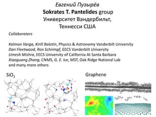
1. Евгений Пузырёв
Sokrates T. Pantelides group
Университет Вандербильт,
Теннесси США
Collaborators
Kalman Varga, Kirill Bolotin, Physics & Astronomy Vanderbilt University
Dan Fleetwood, Ron Schrimpf, EECS Vanderbilt University
Umesh Mishra, EECS University of California At Santa Barbara
Xiaoguang Zhang, CNMS, G. E. Ice, MST, Oak Ridge National Lab
and many more others
SiO2 Graphene

2. 1. Обзор методов вычислительной физики
Много-масштабное моделирование: от дефектов к
ошибкам в приборах
2. Локальная структура металлических сплавов:
диффузионное рассеяние и атомные смещения.
3. Дефекты в полупроводниках и поведение приборов:
GaN, SiC и AlSb.
4. Проблемы функциональности материалов для
мемристора TiO2 и ZnO.
5. Графен,- материал будущего или поиск ниши для
применения.

3. Много-масштабное моделирование
Практическое применение функционала плотности

4. Основные методы
много-масштабного моделирования
I Применение функционала плотности
1. Расчеты возбужденных состояний 10-100 атомов
а) Ширина запрещенной зоны
б) Положение электронного уровня дефекта
LDA+U
Hybrid functional
GW, absorption spectrum T(100 atoms) = 100 000 MPP
2. Расчеты из первых принципов 100-1000 атомов
a) Атомные координаты и электронная
б) Проводимость
LDA (VASP, Quantum ESPRESSO, SIESTA)
II Применение полу-эмпирических потенциалов
Молекулярная динамика и расчеты методом Монте-Карло
10000-1000000 атомов
Классическая механика (LAMMPS, NAMD)

5. Introduction: Ion-Induced Leakage Currents
Metallization burnout after SEGR
Heavy-Ion strikes degrade
or destroy dielectric layers
I-V following biased irradiation of
3.3 nm SiO2 capacitors
Lum, et al., IEEE TNS 51 3263 (2004)
Distinct Electrical degradation modes:
Rupture (Hard breakdown, HB)
Soft breakdown (SB)
Long-term reliability degradation (LTRD)
Massengill, et al., IEEE TNS 48 1904 (2001)

6. Отдача при низких энергиях
TRIM Calculations:
Sample geometry:
Only atomic recoils occurring
IN the SiO2 layer!
High-LET ions generate O(100) eV
recoils in thin oxide layers!

7. Methods
• Quantum Mechanical MD Dynamical atomic and
– DFT-LDA for energy and forces electronic structures
– Classical mechanics for ions
– Cell sizes: 200-1000 atoms Fully QM transport calculations for
underlying transport physics
– Calculation times: 0-1000 fs
• Quantum Mechanical Transport Calculations
– Complex-valued potentials at boundaries as “source” and “sink”
– Non-equilibrium Green’s function method for transport properties
– Orbital basis set: LaGrange functions
• Percolation Theory
– Mott defect-to-defect tunneling
Physically motivated, QM and
– Node-to-node percolation model experimentally parameterized model for
realistic device structures!

8. Много-масштабное моделирование:
От дефектов к ошибкам в приборах
Arbitrary Materials System Arbitrary Device geometry
(~1 nm) (~0.1 micron)
QM Transport
Time-dependent atomic
QM Dynamics
and electronic structure
Percolation Transport
Materials Response
Defect Structure I-V Characteristics
Beck, et al., IEEE TNS
55, 3025 (2008)
Ab Initio calculation of experimentally measureable device properties!

9. Вычислительный Метод
Молекулярная динамика из первых пртципов
• Применение функционала плотности Highest fidelity for bond-
– DFT-LDA for energy and forces
breaking/forming during
low-energy events
• Классическая механика для атомных смещений
• Размер ячейки 200-1000 атомов
• Время 0-1000 fs
Atomic AND electronic structure!
Apply KE to primary atom…
…evolve system!

10. Отдача при низких энергиях
…Correlates with formation of electronic defect states in band gap!
1
0
0 29 58 femtoseconds
after recoil
Beck, et al., IEEE TNS 55, 3025 (2008)

11. Current Results: Multi-scale Model
Arbitrary Materials System Arbitrary Device geometry
(~1 nm) (~0.1 micron)
QM Transport
QM Dynamics
Time-dependent atomic Time-dependent atomic
and electronic structure Percolation and electronic structure
Transport
Materials Response
Defect Structure I-V Characteristics
Beck, et al., IEEE TNS 55,
3025 (2008)
Ab Initio calculation of experimentally measureable device properties!

12. Defect: single oxygen vacancy
EF
defect
Nikolai Sergueev

13. Defect: single oxygen vacancy
2.0
1.5
Current (µA)
EF 1.0
0.5
0
0 0.5 1.0 1.5 2.0
Bias voltage (V)
Transport energy window
from -Vb/2 to +Vb/2
Nikolai Sergueev

14. Amorphous SiO2 leakage currents
Creating defects in a-SiO2
Number of oxygen to be removed:
from 1 to 6
16.24 Å
6 1 3
2
4
5
556 atoms in
scattering region 16.24 Å
Nikolai Sergueev

15. structure
Mol. Dyn. QM Calculations First Principles Transport QM Model
Electrode a-SiO2 Electrode
Theoretical formalism Bias voltage Vb
Tuning the model: crystalline SiO2 system
Leakage currents in thin amorphous SiO2
Nikolai Sergueev

16. Density Functional Theory + “Source and sink” method
Conventional transport methods:
scattering theory, open infinite system
Infinite
… a-SiO2 … system
Our formalism:
K. Varga and S.T. Pantelides,
PRL 98, 076804 (2007) Finite
Source a-SiO2 Sink system
complex potential complex potential
Nikolai Sergueev

17. Flow-chart:
Solve diagonalization problem:
W=Wsource+Wsink
Compute Green’s functions:
Calculate charge density:
Compute leakage current:
Nikolai Sergueev

18. Initial model calculations
Crystalline SiO2 – computationally fast
Al (100) SiO2 Al (100)
d
Can we compute device related property ?
How does conductance of SiO2 depend on oxide thickness d ?
Nikolai Sergueev

19. Conductance versus thickness of SiO2
Not defected
structure yet!
Conductance: exponential dependence as expected from tunneling
Nikolai Sergueev

20. Applying bias voltage across the device …
Calculations Experiment
109
0.54 nm
108
0.8 nm
Current (A/cm2)
107 1.07 nm
106 1.35 nm
1.61 nm
105
104
103
0 0.5 1.0 1.5 2.0
Bias voltage (V)
M. Fukuda et al,
Jpn. J. Appl. Phys. (1998)
We used standard EF
Al Al
Hamiltonian ~ 4.5 eV
SiO2
Nikolai Sergueev

21. Our formalism allows:
--- not only to compute current and conductance
--- but also to analyze the transport mechanism
EF
Oxide states
PDOS – density of states that has an amplitude on oxide atoms
Transmission – describes the tunneling efficiency
Nikolai Sergueev

22. Increasing number of defects …
1 4
Transmission
Transmission
2 5
3 6
Energy (eV) Energy (eV)
Nikolai Sergueev

23. 1 defect
Current (µA)
Bias voltage (V)
Nikolai Sergueev

24. 2 defects
Current (µA)
Bias voltage (V)
Nikolai Sergueev

25. 3 defects
Current (µA)
Bias voltage (V)
Nikolai Sergueev

26. 4 defects
Current (µA)
Bias voltage (V)
Nikolai Sergueev

27. 5 defects
Current (µA)
Bias voltage (V)
Nikolai Sergueev

28. 6 defects
Current (µA)
Bias voltage (V)
Nikolai Sergueev

29. Results: QM Transport Calculations
Al a-SiO2 Al …introduce defect states with specific
energy levels and localizations
QM Tunneling Probability:
Convolution of electronic
Individual defects… DOS and spatial
information
QM calculated I-V characteristics showing
activation of discrete tunneling paths!

30. We performed first principles quantum mechanical
transport calculations and we obtained the following:
conductance vs. oxide thickness dependence is correct
current-voltage dependence qualitatively agrees with experiment
the defects result in the step-like functions of the IV
current increases with number of defects
Going from atomic-scale to mesoscale description …
parameters
First Principles Transport QM Model Percolation Model
Nikolai Sergueev

31. Current Results: Multi-scale Model
Arbitrary Materials System Arbitrary Device geometry
(~1 nm) (~0.1 micron)
QM Transport
QM Dynamics
Time-dependent atomic
and electronic structure
Percolation Transport
Materials Response
Defect Structure I-V Characteristics
Beck, et al., IEEE TNS
55, 3025 (2008)
Ab Initio calculation of experimentally measureable device properties!

32. Results: Percolation Model
Parameterize defect atoms with:
From QM MD calculation Position
Eigenvalue From QM DOS calculation
Defect levels from SHI-induced defects!

33. Mott defect-to-defect tunneling
æ ö é   ù
 
De = çe - e ÷ + qE êe x ×(r - r )ú
i® j è j iø ë j i û
ì
æ   ö
  J = ν0Σij(σiboundary-σj)
ï ç- r -r ÷
ï
ï exp ç j i ÷, De £0
ç r ÷ i® j ν0 = 1.15 × 1013 s–1
ï ç ÷
ï è 0
ø
P =í
i® j ï æ  
  ö
ï ç- r -r -De ÷
i® j÷
ï exp ç j i
+ , De >0
ï ç r kT ÷ ÷ i® j
ï ç 0
è ø
î
é æ ö æ ö ù
j j
å
s s + 1 = s s + ês s ç1- s s ÷ P
ë i è jø i® j
- s s ç1- s s ÷ P
jè
ú
i ø j ® iû
i
ri – defect position
Defects
E – external field
DOS εi - energy level relative to EF
σi – site occupancy, [0, 1], at boundary σ=0.5
ν0- Mott’s escape frequency
Iterative procedure for occupancies until Δσi < 10-7
S. Simeonov et al. Physica Status Solidi, 13, 2004

34. Defect-to-defect tunneling
• L =1.4 nm Defects DOS
• Defect energy levels
• Defect atomistic map ri, εi ,σi
time = 78fs
22 defects
L
E

35. Defect-to-defect tunneling
ri, εi ,σi

36. Leakage Current Temperature Dependence
4 2
Current, nA
-2 0-4
-6
-20.0 -10.0 0.0 10.0 20.0
qE, MV/cm

37. Leakage Current Time Dependence
6 4
Current, nA
2 0
-2
-10.0 -5.0 0.0 5.0 10.0 15.0 20.0
qE, MV/cm

38. Model results in real-time
defect evolution and transient currents

39. Defect time evolution
10 15 20 25
Number of defects
Energy
Space
5
Transient current
Current, nA
0.0 4.0 8.0
Keeps going
0 200 400 500 600
time, fs

40. Results: Calculated I-V Characteristics
4
Thermal smoothing
2
Current, nA
0
Asymmetric: Defect Steps showing activation of
level dependence discrete tunneling paths
-2 -4
-6
-20 -10 0.0 10 20
qE, MV/cm

41. Results: Transient I-V Characteristics
6 fs 32 fs 58 fs
Thresholds in time and applied field!

42. Results: Transient Leakage
Defects and current peaks Defects and current persists
within ~200 fs of recoil on the ns time-scale
E=3 V
E=1.5 V Roughness of curve due to
exponential dependence on atomic
and electronic structure!
Transient defect-induced weakness!

43. As a result of the calculation
we have direct comparison
with experiment for the gate
current as a function of gate
voltage!
Quantitative
agreement!
Massengill, et al., IEEE TNS 48 1904 (2001)

44. Graphene device degradation
• Graphene fabricated by mechanical
exfoliation from Kish graphite
• Sweep VG with VDS=5mV

45. Motivation and Outline
 Experiment [1]
o Graphene’s resistivity response to x-ray radiation,
ozone exposure, annealing.
o Defect related Raman D-peak appears after
 x-ray irradiation in air
 ozone exposure, decreases after annealing.
 Theory: behavior of impurities on graphene
o Temperature and concentration dependence.
o Need to remove oxygen without vacancy formation (would H help?)
[1] E.-X. Zhang et al, IEEE Trans. Nucl. Sci. 58, 2961 (2011)

46. Graphene device degradation
Two-probe resistances measured on
• 10 keV irradiated graphene
• pristine graphene
• ozone exposed graphene (1 min)
• annealed (300C for 2 hrs in 200 sccm Ar)

47. Graphene device degradation
Ozone exposure
a) 80
8000
60
Integrated intensity Area
G-Peak
6000
ID/IG (100%)
40 Defect related D-peak
4000
20 • increases x-ray exposure
2000
D-Peak • decreases after temperature anneal
0 0
Pre 8 Mrad(SiO2) 15 Mrad(SiO2) Anneal
10-keV X-ray Dose
b)

48. Theoretical Approach
O O desorption Density Functional Theory
O migration DFT
• Defect formation energies
• Migration/desorption barriers
O dimer
Kinetic Monte-Carlo
KMC
Defect dynamics
• Temperature
• Initial concentration

49. Oxygen Removal and Vacancy Generation
1.3 eV Oxygen: clustering behavior
0.5 eV
0.8 eV Removal of oxygen
Bridge 1.3 eV • Pairs O2
• Triplets CO, CO2, VC
Top
Device degradation
1.1 eV CO, CO2 1.1 eV O2

50. High-temperature Annealing
Vacancy
Concentration of vacancies exceeds
Residual oxygen atom concentration of residual O

51. High vs Low Temperature Anneal
T, oC
T

52. Temperature Anneal
Initial Defect Concentration Dependence
High O concentration
Lo
vacancy
surface coverage
Low O, High V concentration
oxygen
T
initial O surface coverage
High T: Removal of oxygen > 0.05 initial surface coverage leads to vacancy formation
Low T: Oxygen stays on the surface and forms clusters
Decrease of D-peak, Increase in resistivity
Method to prevent defect formation during irradiation/annealing?

53. Oxygen and Hydrogen on Graphene:
Binding energies, Migration and Reaction Barriers
O-H is most likely to desorb
O from graphene surface
H
Leaves carbon network intact

54. Effect of Hydrogen On
Oxygen Annealing
Oxygen/Hydrogen Low High
Concentrations
Low 2% O, 10% H
@ T = 300 C
Final defect
concentrations?
High 15% O, 1% H 15% O, 10% H

55. Effect of Hydrogen On Oxygen Annealing
Higher Oxygen concentration Higher Hydrogen concentration
Hydrogen is removed t ~ 0.001 s Oxygen is removed t ~ 0.0001 s
t~1s t~1s
Removal of residual Oxygen Residual Hydrogen
Causes formation of large Forms clusters L ~ 0.5 nm
amount of Vacancies No Vacancies are formed

56. High O, High H concentrations
Hydrogen is removed first,
Removal of residual Oxygen
Causes formation of Vacancies
Effect of Hydrogen On Oxygen Annealing

57. Электронная плотность
Разложение по функциям Гаусса
  æ q ö
   

r r =()
N atoms
å
 
(

rn r - Rn ) ( ) (
rn r - Rn = ç1- n ÷ r0A r - Rn
ç Q ÷
è Aø
)
n=1
Перенос заряда
 M gauss
()
rn r = hr å cme
2 -g m r 2
m=1
  
ò
Wcell
( )
rn r - Rn d 3r = QA - qn
*

58. Полная энергия
   
Etotal =
W
ò é
ë () ()
W r êr r
ù
ú
û W
ê
ë () ()
r r d 3r + ò W q ér q ù r q d 3q + Eion-ion
ú
û
volume volume
  
é
W r êr r
ë () ù é
ú = T êr r
û ë () ù
ú
û
é
()ù
+Vex êr r ú
ë û
  
é ù
()
W q êr q ú =Vps q +Vhartree q
ë û () () Vps q S q wpseudo q

59. Кинетическая энергия
corr corr
T TWang Teter TLDA Tatom
    5 
é
() ù 45
( ) () ( ) ( )
2
òò
5
TWang-Teter êr r ú = 3p 2 3
r 6 r w1 r - r ' r 6 r ' d 3rd 3r '-
ë û 128
  
( ) () () ()
2
ò r 3 r d r - ò r 2 r Ñ r 2 r d 3r
21 5 1 1 1
- 3p 2 3 3 2
250 2
Теория линейного отклика
5 1 3 2 3 1 q2 4 2 q
w1 w q q , and w ln
8 4 5 2 8q 2 q

60.  ì6
N grid  ü
() ()
ï ï
TLDA ér r ù=
å íåcnDr ri ý
n
corr 2
ê
ë ú
û i=1 ï n=1
î ï
þ
3
6 æp ö 2 æ k2 ö
()
Tatom k = å cn ç ÷ exp ç -
corr
çx ÷
è nø
ç 4x ÷
è
÷
n=1 nø


 æ k ö  

()
S A ki = å ç1- a ÷ exp -ika iRa
ç N ÷
a ÎA è a ø
( )

61. λ=1 upper limit von Weizsäcker
λ=1/9 gradient expansion second order
λ=1/5 computational Hartree-Fock

62. 1. Phase Diagram
2. Elastic Properties
3. Defect Formation Energies

63. Ширина запрещенной зоны
G0W0 GaN