This document discusses key concepts in sampling and population parameter estimation including:
1) How sample size, mean, and standard deviation relate to estimating population mean and determining appropriate distributions.
2) How sample size, proportion, and standard deviation relate to estimating population proportion.
3) The chi-square distribution and how it relates to estimating population variance.
4) How to determine minimum sample size needed based on desired accuracy of estimates.
5) Several example problems are provided to illustrate concepts.
The ppt gives an idea about basic concept of Estimation. point and interval. Properties of good estimate is also covered. Confidence interval for single means, difference between two means, proportion and difference of two proportion for different sample sizes are included along with case studies.
The ppt gives an idea about basic concept of Estimation. point and interval. Properties of good estimate is also covered. Confidence interval for single means, difference between two means, proportion and difference of two proportion for different sample sizes are included along with case studies.
1. (2 points)Two random samples are selected from two indepe.docxSONU61709
1. (2 points)
Two random samples are selected from two independent pop-
ulations. A summary of the samples sizes, sample means, and
sample standard deviations is given below:
n1 = 37, x̄1 = 52.4, s1 = 5.8
n2 = 48, x̄2 = 75, s2 = 10
Find a 92.5% confidence interval for the difference µ1− µ2
of the means, assuming equal population variances.
Confidence Interval =
Answer(s) submitted:
•
(incorrect)
2. (2 points) In order to compare the means of two popu-
lations, independent random samples of 238 observations are
selected from each population, with the following results:
Sample 1 Sample 2
x1 = 1 x2 = 3
s1 = 120 s2 = 200
(a) Use a 97 % confidence interval to estimate the difference
between the population means (µ1−µ2).
≤ (µ1−µ2)≤
(b) Test the null hypothesis: H0 : (µ1− µ2) = 0 versus the al-
ternative hypothesis: Ha : (µ1− µ2) 6= 0. Using α = 0.03, give
the following:
(i) the test statistic z =
(ii) the positive critical z score
(iii) the negative critical z score
The final conclustion is
• A. We can reject the null hypothesis that (µ1−µ2) = 0
and accept that (µ1−µ2) 6= 0.
• B. There is not sufficient evidence to reject the null hy-
pothesis that (µ1−µ2) = 0.
(c) Test the null hypothesis: H0 : (µ1−µ2) = 26 versus the al-
ternative hypothesis: Ha : (µ1−µ2) 6= 26. Using α = 0.03, give
the following:
(i) the test statistic z =
(ii) the positive critical z score
(iii) the negative critical z score
The final conclustion is
• A. We can reject the null hypothesis that (µ1−µ2) = 26
and accept that (µ1−µ2) 6= 26.
• B. There is not sufficient evidence to reject the null hy-
pothesis that (µ1−µ2) = 26.
Answer(s) submitted:
•
•
•
•
•
•
•
•
•
•
(incorrect)
3. (2 points) Two independent samples have been selected,
70 observations from population 1 and 83 observations from
population 2. The sample means have been calculated to be
x1 = 14.9 and x2 = 10.5. From previous experience with these
populations, it is known that the variances are σ21 = 20 and
σ22 = 21.
(a) Find σ(x1−x2).
answer:
(b) Determine the rejection region for the test of H0 :
(µ1−µ2) = 2.92 and Ha : (µ1−µ2)> 2.92 Use α = 0.05.
z >
(c) Compute the test statistic.
z =
The final conclustion is
• A. We can reject the null hypothesis that (µ1− µ2) =
2.92 and accept that (µ1−µ2)> 2.92.
• B. There is not sufficient evidence to reject the null hy-
pothesis that (µ1−µ2) = 2.92.
(d) Construct a 95 % confidence interval for (µ1−µ2).
≤ (µ1−µ2)≤
Answer(s) submitted:
•
•
•
•
•
•
(incorrect)
4. (2 points) Randomly selected 100 student cars have ages
with a mean of 7.2 years and a standard deviation of 3.4 years,
while randomly selected 85 faculty cars have ages with a mean
of 5.4 years and a standard deviation of 3.3 years.
1
1. Use a 0.01 significance level to test the claim that student
cars are older than faculty cars.
The test statistic is
The critical value is
Is there sufficient evidence to support the claim that student
cars are older than faculty cars?
• A. Yes
• ...
Please Subscribe to this Channel for more solutions and lectures
http://www.youtube.com/onlineteaching
Chapter 7: Estimating Parameters and Determining Sample Sizes
7.2: Estimating a Population Mean
Please Subscribe to this Channel for more solutions and lectures
http://www.youtube.com/onlineteaching
Chapter 7: Estimating Parameters and Determining Sample Sizes
7.2: Estimating a Population Mean
Esitmates for year 201620162015Sales (units) increase.docxYASHU40
Esitmates for year 2016
2016
2015
Sales (units) increase
10%
115,000
Sale Price (unit) increase
1%
$5.00
Raw material:
Price
DM - Plasitic (lb.)
$2.90
$3.00
DM - Wheel (wheel)
$0.03
$0.02
Labor cost:
wage rate (airplane)
$0.60
$88,775
total
MOH:
Indirect material (per airplane)
$0.005
Indirect labor (per airplane)
$0.003
utility
$850
factory depreciation
$1,000
$27,000
total
Period cost:
S&A expenses - variable (per airplane)
$0.01
S&A expenses - Fixed
$15,000
$130,000
total
Finished Goods:
beginning (units)
?
desired ending (units)
9%
of yearly sales
15,000
Account receivable
25%
23%
Account payable
25%
23%
Tax rate
30%
30%
Minimun bank account
$50,000
$50,000
What is the break-even in sales units for 2016?
What is the target sale in sales units for 2016 with a target profit of $200,000?
Assuming at the beginning of 2015, the company made the plan same as 2016. Find the quantity factors and price factors for 2015:
Prepare income statement using both variable costing method and absorption costing method for 2016
Prepare a flexible budget for 2016, with decrease 10% sales, same, and increase 10% sales
Prepare a Master Budget for 2016:
Sales budget
Production budget
DM purchases budget
DL cost budget
MOH cost budget
COGS budget
S&A budget
Cash budget
Account receivable
Account payable
Does the factory need to borrow money at the end of 2016?
MS1023 Business Statistics with Computer Applications Homework #4
Maho Sonmez [email protected] 1
MS1023 Business Statistics w/Comp Apps I
Homework #4 – Use Red Par Score Form
Chps. 9 & 10: 50 Questions Only
1. The first step in testing a hypothesis is to
establish a true null hypothesis and a false
alternative hypothesis.
a) True
b) False
2. In testing hypotheses, the researcher
initially assumes that the alternative
hypothesis is true and uses the sample data
to reject it.
a) True
b) False
3. The null and the alternative hypotheses
must be mutually exclusive and collectively
exhaustive.
a) True
b) False
4. Generally speaking, the hypotheses that
business researchers want to prove are stated
in the alternative hypothesis.
a) True
b) False
5. When a true null hypothesis is rejected,
the researcher has made a Type I error.
a) True
b) False
6. When a false null hypothesis is rejected,
the researcher has made a Type II error.
a) True
b) False
7. The rejection region for a hypothesis test
becomes smaller if the level of significance
is changed from 0.01 to 0.05.
a) True
b) False
8. Whenever hypotheses are established
such that the alternative hypothesis is "μ>8",
where μ is the population mean, the
hypothesis test would be a two-tailed test.
a) True
b) False
9. Whene ...
I am Paul G. I am a Data Analysis Assignment Expert at excelhomeworkhelp.com. I hold a Master's in Statistics, from Queensland, Australia. I have been helping students with their assignments for the past 10 years. I solved assignments related to Data Analysis.
Visit excelhomeworkhelp.com or email info@excelhomeworkhelp.com. You can also call on +1 678 648 4277 for any assistance with Data Analysis Assignment.
Check your solutions from the practice. Please be sure you f.docxspoonerneddy
Check your solutions from the practice. Please be sure you fully understand all
solutions before taking your exam.
1 . a. The type of study is observational with the variable of interest being the
age of the student.
2 . (41.1, 50.9)
3. a. 36 movies
b . 29 movies
c. 23 movies
d. About 230 minutes
4. Part a: Median 139,500 Mean: 163,125
Part b: Outlier 34,000 Median: 140,000 Mean: 182, 000
Part c: outlier 434,000 Median: 139,000 Mean: 124,428.57
5 . a. The goal is to determine how many teachers would choose a different
career if given the opportunity
b . All US teachers
c. Percentage of teachers who would choose a different career
d. 2150 teachers who were questioned
e . Raw data is teacher responses (yes no) to question if they would choose a
different career.
f. 60% of teachers who said they would choose a different career
g. 55%---65%
6. Red: (0.85,0.97)
Yellow: (0.86, 0.98)
Blue: (0.86,0.94)
7 . F ro m st at di sk
Source: DF: SS: MS: Test Stat, F: Critical F: P---Value:
Treatment: 2 0.00224 0.00112 0.505269 6.112108 0.612123
Error: 17 0.03769 0.002217
Total: 19 0.03993
Fail to Reject the Null Hypothesis
There is not sufficient evidence to reject equality of means
The p value 0.61
We have sufficient evidence to claim the mean of all colors is the same.
8. Expected probability of rolling a 2: 0.16
Actual results: 0.44
Difference 0.28, this is statistically significant
9 . Null hypothesis: The mean of all three players are the same
Alternative hypothesis: the mean of at least one player is different
The p value is 0.036
At this level we must reject Ho and conclude at least one mean is statistically
different.
1 0 . The minimum sample size is 365 students
1 1 . a. 58%
b . 74%
c. 82%
d . 7 8
1 2 . H0: p=0.095
a. Ha: P<---.095
b . P hat= 0.0920
c. Z=---0.33
d. No
Test results from stat disk are as follows:
Claim: p < p(hyp)
Sample proportion: 0.0920304
Test Statistic, z: ---0.3288
Critical z: ---1.6449
P---Value: 0.3712
90% Confidence interval:
0.0773847 < p < 0.106676
Fail to Reject the Null Hypothesis
Sample does not provide enough evidence to support the claim
1 3 . a. 2 standard deviations
b . 97.72%
1 4. FROM STAT DISK:
Descriptive Statistics
Column 3
Sample Size, n: 15
Mean:8.2
Median: 8
Midrange: 8.5
RM S : 8.306624
Variance, s^2: 1.885714
St Dev, s:1.373213
Mean Abs Dev: 1.066667
Range: 5
Coeff. Of Var. 16.75%
Minimum: 6
1 st Quartile: 7
2 nd Quartile: 8
3 rd Quartile: 9
Maximum: 11
Sum: 123
Sum Sq: 1035
c. The best estimate for the mean is 8.2 people
d. The 95% confidence interval is (from stat disk)
Margin of error, E = 0.7586815
95% Confident the population mean is within the range:
7. 44 1 3 1 9 < mean <8.958681
No this is not representative of the entire nation
1 5 . Type I error: reject the fact that males and females are equal in GPA when
that is in fact true
Type II error--- Conclude the GPA of males .
Show drafts
volume_up
Empowering the Data Analytics Ecosystem: A Laser Focus on Value
The data analytics ecosystem thrives when every component functions at its peak, unlocking the true potential of data. Here's a laser focus on key areas for an empowered ecosystem:
1. Democratize Access, Not Data:
Granular Access Controls: Provide users with self-service tools tailored to their specific needs, preventing data overload and misuse.
Data Catalogs: Implement robust data catalogs for easy discovery and understanding of available data sources.
2. Foster Collaboration with Clear Roles:
Data Mesh Architecture: Break down data silos by creating a distributed data ownership model with clear ownership and responsibilities.
Collaborative Workspaces: Utilize interactive platforms where data scientists, analysts, and domain experts can work seamlessly together.
3. Leverage Advanced Analytics Strategically:
AI-powered Automation: Automate repetitive tasks like data cleaning and feature engineering, freeing up data talent for higher-level analysis.
Right-Tool Selection: Strategically choose the most effective advanced analytics techniques (e.g., AI, ML) based on specific business problems.
4. Prioritize Data Quality with Automation:
Automated Data Validation: Implement automated data quality checks to identify and rectify errors at the source, minimizing downstream issues.
Data Lineage Tracking: Track the flow of data throughout the ecosystem, ensuring transparency and facilitating root cause analysis for errors.
5. Cultivate a Data-Driven Mindset:
Metrics-Driven Performance Management: Align KPIs and performance metrics with data-driven insights to ensure actionable decision making.
Data Storytelling Workshops: Equip stakeholders with the skills to translate complex data findings into compelling narratives that drive action.
Benefits of a Precise Ecosystem:
Sharpened Focus: Precise access and clear roles ensure everyone works with the most relevant data, maximizing efficiency.
Actionable Insights: Strategic analytics and automated quality checks lead to more reliable and actionable data insights.
Continuous Improvement: Data-driven performance management fosters a culture of learning and continuous improvement.
Sustainable Growth: Empowered by data, organizations can make informed decisions to drive sustainable growth and innovation.
By focusing on these precise actions, organizations can create an empowered data analytics ecosystem that delivers real value by driving data-driven decisions and maximizing the return on their data investment.
Techniques to optimize the pagerank algorithm usually fall in two categories. One is to try reducing the work per iteration, and the other is to try reducing the number of iterations. These goals are often at odds with one another. Skipping computation on vertices which have already converged has the potential to save iteration time. Skipping in-identical vertices, with the same in-links, helps reduce duplicate computations and thus could help reduce iteration time. Road networks often have chains which can be short-circuited before pagerank computation to improve performance. Final ranks of chain nodes can be easily calculated. This could reduce both the iteration time, and the number of iterations. If a graph has no dangling nodes, pagerank of each strongly connected component can be computed in topological order. This could help reduce the iteration time, no. of iterations, and also enable multi-iteration concurrency in pagerank computation. The combination of all of the above methods is the STICD algorithm. [sticd] For dynamic graphs, unchanged components whose ranks are unaffected can be skipped altogether.
Explore our comprehensive data analysis project presentation on predicting product ad campaign performance. Learn how data-driven insights can optimize your marketing strategies and enhance campaign effectiveness. Perfect for professionals and students looking to understand the power of data analysis in advertising. for more details visit: https://bostoninstituteofanalytics.org/data-science-and-artificial-intelligence/
Innovative Methods in Media and Communication Research by Sebastian Kubitschk...
06 sampling
1. INTERNATIONAL UNIVERSITY (IU) Engineering Probability & Statistic
ISE Department Lecturer: Phan Nguyễn Kỳ Phúc
--------------------o0o------------------
06 Sampling 1
SAMPLING
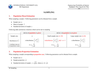
1. Population Mean Estimation
When sampling a sample, 3 following parameters can be obtained from a sample
Sample size: n
Mean of sample: x
Standard deviation of sample: s
Following table summarizes situations which can be met in sampling
std (σ) of population is given std (σ) of population is not given
Sample size: n Small sample size (n<30) Large sample size (n≥30)
Distribution of x z-distribution:
2
,x
n
t-distribution:
2
,
s
x
n
, 1dof n z-distribution:
2
,
s
x
n
Confident interval
of population mean 2
x z
n
, 1
2
n
s
x t
n
2
s
x z
n
2. Population Proportion Estimation
When sampling a sample corresponding to proportion case, 3 following parameters can be obtained from a sample
Sample size: n
Sample proportion: p
Standard deviation of sample: , where (1 )s pq q p
2. INTERNATIONAL UNIVERSITY (IU) Engineering Probability & Statistic
ISE Department Lecturer: Phan Nguyễn Kỳ Phúc
--------------------o0o------------------
06 Sampling 2
Population Proportion Estimation (cont.)
std (σ) of population is given
Sample size: n
Distribution of p z-distribution:
,
pq
p
n
CI of population
proportion
2
pq
x z
n
3. The Chi-Square χ2
Distribution & Population Variance Estimation
The chi-square distribution is NOT SYMMETRIC
The chi-square distribution is used to TEST the VARIANCE
The chi-square distribution requires the DEGREE OF FREEDOM (dof)
std (σ) of population is given
Sample size: n
Distribution of
2
2
( 1)n s
χ2
-distribution: 1dof n
CI of population variance
2 2
2 2
, 1 1 , 1
2 2
( 1) ( 1)
,
n n
n s n s
4. Sample Size Determination
We want to increase the accuracy in estimating the populations mean up to certain level =>
decrease the width of CI
Width of CI:
2
2 2z B
n
So given a bound B, MINIMUM SAMPLE SIZE must satisfy:
2 2
/2
2
2
z
z B n
Bn
3. INTERNATIONAL UNIVERSITY (IU) Engineering Probability & Statistic
ISE Department Lecturer: Phan Nguyễn Kỳ Phúc
--------------------o0o------------------
06 Sampling 3
Assignments
Question 1: Suppose you are sampling from a population with mean µ= 1,065 and standard
deviation σ = 500. The sample size is n=100. What are the expected value and the variance of
the sample mean ?
Question 2: Suppose you are sampling from a population with population variance σ2
=
1,000,000. You want the standard deviation of the sample mean to be at most 25. What is the
minimum sample size you should use?
Question 3: When sampling is from a population with mean 53 and standard deviation 10, using
a sample of size 400, what are the expected value and the standard deviation of the sample mean?
Question 4: What are the expected value and the standard deviation of the sample
proportion if the true population proportion is 0.2 and the sample size is n= 90.
Question 5: Häagen-Dazs ice cream produces a frozen yogurt aimed at health-conscious ice
cream lovers. Before marketing the product in 2007, the company wanted to estimate the
proportion of grocery stores currently selling Häagen-Dazs ice cream that would sell the new
product. If 60% of the grocery stores would sell the product and a random sample of 200 stores
is selected, what is the probability that the percentage in the sample will deviate from the
population percentage by no more than 7 percentage points?
Question 6: Japan’s birthrate is believed to be 1.57 per woman. Assume that the population
standard deviation is 0.4. If a random sample of 200 women is selected, what is the probability
that the sample mean will fall between 1.52 and 1.62?
Question 7: A real estate agent needs to estimate the average value of a residential property of a
given size in a certain area. The real estate agent believes that the standard deviation of the
property values is σ = $5,500.00 and that property values are approximately normally distributed.
A random sample of 16 units gives a sample mean of $89,673.12. Give a 95% confidence
interval for the average value of all properties of this kind.
Question 8: An astronomer wants to measure the distance from her observatory to a distant star.
However, due to atmospheric disturbances, any measurement will not yield the exact distance d.
As a result, the astronomer has decided to make a series of measurements and then use their
average value as an estimate of the actual distance. If the astronomer believes that the values of
the successive measurements are independent random variables with a mean of d light years and
a standard deviation of 2 light years, how many measurements need she make to be at least 95
percent certain that her estimate is accurate to within ± .5 light years?