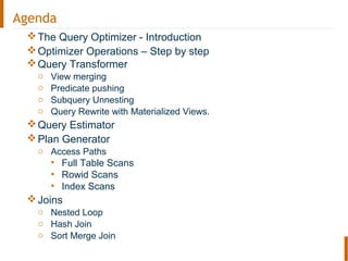
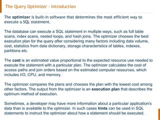
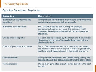
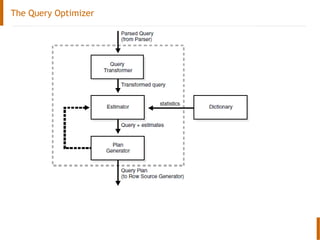
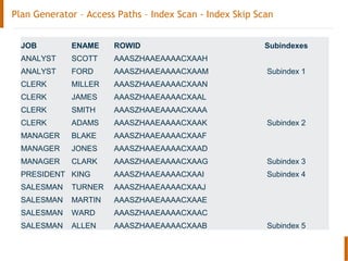
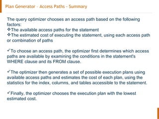
The document discusses the Oracle query optimizer. It describes the key components and steps of the optimizer including the query transformer, query estimator, and plan generator. The query transformer rewrites queries for better performance through techniques like view merging, predicate pushing, and subquery unnesting. The query estimator calculates selectivity, cardinality, and cost to determine the overall cost of execution plans. The plan generator explores access paths, join methods, and join orders to select the lowest cost plan.

1. Technical Skills Enhancement – PL/SQL Best
practices
Query Optimizer

2. Objectives
At the end of this training, you will be able to:
• Understand the workings of query optimizer
• Write better performing queries

3. Agenda
The Query Optimizer - Introduction
Optimizer Operations – Step by step
Query Transformer
o View merging
o Predicate pushing
o Subquery Unnesting
o Query Rewrite with Materialized Views.
Query Estimator
Plan Generator
o Access Paths
• Full Table Scans
• Rowid Scans
• Index Scans
Joins
o Nested Loop
o Hash Join
o Sort Merge Join

4. The Query Optimizer - Introduction
The optimizer is built-in software that determines the most efficient way to
execute a SQL statement.
The database can execute a SQL statement in multiple ways, such as full table
scans, index scans, nested loops, and hash joins. The optimizer chooses the best
execution plan for the query after considering many factors including data volume,
cost, statistics from data dictionary, storage characteristics of tables, indexes,
partitions etc.
The cost is an estimated value proportional to the expected resource use needed to
execute the statement with a particular plan. The optimizer calculates the cost of
access paths and join orders based on the estimated computer resources, which
includes I/O, CPU, and memory.
The optimizer compares the plans and chooses the plan with the lowest cost among
other factors. The output from the optimizer is an execution plan that describes the
optimum method of execution.
Sometimes, a developer may have more information about a particular application's
data than is available to the optimizer. In such cases hints can be used in SQL
statements to instruct the optimizer about how a statement should be executed.

5. The Query Optimizer
Optimizer Operations – Step by step
Operation Description
Evaluation of expressions and
conditions
The optimizer first evaluates expressions and conditions
containing constants as fully as possible.
Statement transformation For complex statements involving, for example,
correlated subqueries or views, the optimizer might
transform the original statement into an equivalent join
statement.
Choice of access paths For each table accessed by the statement, the optimizer
chooses one or more of the available access paths to
obtain table data.
Choice of join types and orders For an SQL statement that joins more than two tables,
the optimizer chooses which pair of tables is joined first,
and then which table is joined to the result, and so on.
Cost Estimation The optimizer calculates COST of the query, taking into
consideration all the data collected from the above steps
Plan generation Oracle then generates execution plan based on the cost,
join etc.

6. The Query Optimizer

7. Query Transformer

8. Query Transformer
The Query Transformer determines whether it is advantageous
to rewrite the query into a semantically equivalent query that
performs better than the original query.
It then rewrites the query if needed.
This is additional overhead, but it speeds up the overall
processing of the query than executing a complex query that
contains unnecessary views, subqueries, additional processing
etc.
So it is always a better practice to
- choose base tables over views
- choose joins over subqueries

9. Query Transformer
Query Block
Each query portion of a statement is called a query block.
The input to the query transformer is a parsed query, which is represented
by a set of query blocks.
In the following example, the SQL statement consists of two query blocks.
The subquery in parentheses is the inner query block. The outer query
block, is the rest of the SQL statement.

10. Query Transformer
The query transformer employs several query transformation techniques, including
the following:
•View Merging
•Predicate pushing
•Subquery Unnesting
•Query Rewrite with Materialized Views.
View Merging –
Each view referenced in a query is expanded by the parser into a separate query
block.
This provides better performance.
Without view merging Oracle would have to execute the query behind the view
separately with its own execution subplan and then feed the results to the main
query. This takes more time than view merging.
The view merging optimization applies to simple views that contain only selections,
projections, and joins. That is, mergeable views do not contain set operators,
aggregate functions, DISTINCT, GROUP BY, CONNECT BY, and so on…..

11. Query Transformer– View merging
For example, suppose you create a view as follows:
CREATE or replace VIEW emp_30_vw AS
SELECT empno, ename, job, sal, deptno
FROM emp
WHERE deptno = 30;
Then execute a query on the view as below
SELECT empno
FROM emp_30_vw
WHERE empno > 150;
Oracle’s statement transformer rewrites the query as below
SELECT empno, ename, job, sal, deptno
FROM emp
WHERE deptno = 30
AND empno >150;
A better idea would be to eliminate the view from the query and use base
tables

12. Query Transformer– Predicate Pushing
Predicate Pushing
For complex views that contain set operators, aggregate functions, DISTINCT,
GROUP BY, CONNECT BY, and so on, Oracle employs another technique called
Predicate Pushing to improve performance.
In predicate pushing, the optimizer "pushes" the relevant predicates from the
containing query block into the view query block
This technique improves the subplan of the unmerged view because the database
can use the pushed-in predicates to access indexes or to use as filters.

13. Query Transformer– Predicate Pushing
For example, suppose you create a view that references two employee tables. The
view is defined with a compound query that uses the UNION set operator, as
follows:
CREATE OR REPLACE VIEW all_emp_vw AS
( SELECT ename, empno, deptno
FROM emp )
UNION
( SELECT ename, empno, deptno
FROM emp_b )
You then query the view as follows:
SELECT ename
FROM all_emp_vw
WHERE deptno= 10;

14. Query Transformer– Predicate Pushing
The optimizer can transform the accessing statement by pushing its predicate, the
WHERE clause condition deptno=10, into the view's compound query. The
equivalent transformed query is as follows:
SELECT ename from
( SELECT ename, empno, deptno
FROM emp
WHERE deptno = 10)
UNION
( SELECT ename, empno, deptno
FROM emp_b
WHERE deptno = 10)

15. Query Transformer– Subquery unnesting
Subquery unnesting
In subquery unnesting, the optimizer transforms a nested query into an equivalent
join statement, and then optimizes the join.
Joins are generally faster than their equivalent subqueries.
The optimizer can perform this transformation only if the resulting join statement
is guaranteed to return exactly the same rows as the original statement, and if
subqueries do not contain aggregate functions .
Suppose you run a query as below -
SELECT *
FROM emp
WHERE deptno
IN (SELECT deptno FROM dept WHERE dname ='ACCOUNTING');
Script : SubQuery_Unnesting.sql
Without subquery unnesting, the inner query block will be executed first with its
own execution plan and then the outer query block with a separate query plan.

16. Query Transformer– Subquery unnesting
. Inner Query Block
Outer Query Block

17. Query Transformer– Subquery unnesting
.
Execution plan of query with subquery

18. Query Transformer– Subquery unnesting
.
Execution plan of query with join

19. Query Transformer- Query Rewrite with Materialized Views
Materialized Views
A materialized view is a database object that physically stores the result of a
query.
It was originally introduced in Oracle 8i as an extension of snapshots
The data stored in an Mview has to be refreshed in order to be in sync with real
time transactional data. Oracle provides 3 options for this- time criteria, upon
commit of changes, or upon demand.
Mview provides substantial performance gains in some cases since the query is run
only once rather than for each repeated use.
Script : MaterializedView.sql

20. Query Transformer- Query Rewrite with Materialized Views
Query Rewrite with Materialized Views
•Oracle Enterprise Edition offers a statement transformation feature called “Query Rewrite”
that rewrites the query if it finds that there is an equivalent materialized view with the same
query blocks as the original query
•11g product comparisons
Database-11g-product-family-technic-133664.pdf
•12 C product comparisons
http://www.oracle.com/us/products/database/enterprise-edition/comparisons/index.html

21. Query Estimator

22. Query Estimator
The Query estimator determines the overall cost of a given execution plan. The
estimator generates three different types of measures to achieve this goal. If statistics
are available, then the estimator uses them to compute the measures. The statistics
improve the degree of accuracy of the measures.
•Selectivity
This measure represents the fraction of rows that will be selected by a query
predicate, from a row set.
•Cardinality
This measure represents the number of rows selected from a row set by a join or a
query predicate.
•Cost
This measure represents units of work or resource used. The query optimizer uses
disk I/O, CPU usage, and memory usage as units of work (for scanning a table,
accessing rows from a table by using an index, joining two tables together, filtering
rows using predicates, sorting a row set, grouping data etc)

23. Plan Generator

24. Plan Generator
The plan generator explores various plans for a query block by trying out different
access paths, join methods, and join orders. Many plans are possible because of the
various combinations of the above mentioned items. The goal of the plan generator is
to choose the plan with the lowest cost.
Access Paths
Access paths are ways in which data is retrieved from the database. In general, index
access paths are useful for statements that retrieve a small subset of table rows,
whereas full scans are more efficient when accessing a large portion of the table.
Join Methods
To join each pair of row sources, Oracle Database must perform a join operation. Join
methods include nested loop, sort merge and hash joins.
To execute a statement that joins more than two tables, Oracle Database joins two of
the tables and then joins the resulting row source to the next table. This process
continues until all tables are joined into the result.

25. Plan Generator – Access Paths
• Online transaction processing (OLTP) applications, which consist of short-running
SQL statements with high selectivity, often are characterized by the use of index
access paths.
• Decision support systems, Reports and Data warehouses however, tend to
perform full table scans of the relevant partitions.
• The data access paths that Oracle can use to locate and retrieve any row in any
table are below -
– Full Table Scans
– Rowid Scans
– Index Scans

26. Plan Generator – Access Paths – Full Table Scan
Full table Scan
•This type of scan reads almost all rows from a table and filters out only a few records
that do not meet the selection criteria.
•During a full table scan, all blocks in the table are scanned.
•Each row is examined to determine whether it satisfies the statement's WHERE
clause.
•When Oracle Database performs a full table scan, the blocks are read sequentially.
•Because the blocks are adjacent, the database can make I/O calls larger than a
single block to speed up the process.

27. Plan Generator – Access Paths – Full Table Scan
Why a Full Table Scan Is Faster for Accessing Large Amounts of Data
•Full table scans are slightly cheaper than index range scans when accessing a large
fraction of the blocks in a table.
•Full table scans can use larger I/O calls, and making (a few) large I/O calls is
cheaper than making many smaller calls..

28. Plan Generator – Access Paths – Full Table Scan
When does the Optimizer use Full Table Scans
The optimizer uses a full table scan in any of the following cases:
Lack of Index
If the query cannot use existing indexes, then it uses a full table scan. For example, if
there is a function used on the indexed column in the query, then the optimizer
cannot use the index and instead uses a full table scan.
Large Amount of Data
If the optimizer thinks that the query requires most of the blocks in the table, then it
uses a full table scan, even though indexes are available.
Small Table
If a table contains less blocks than what the database can read in a single I/O call,
then a full table scan might be cheaper than an index range scan, regardless of the
fraction of rows being accessed or indexes present.
Script : FullTableScan.sql

29. Plan Generator – Access Paths – Rowid Scan
• The rowid of a row specifies the data file and data block containing the row and
the location of the row in that block.
• Locating a row by specifying its rowid is the fastest way to retrieve a single row,
because the exact location of the row in the database is specified.
• In general, indexes store the values of indexed columns along with the rowid of
the table’s row.
• To access a table by rowid, Oracle Database first obtains the rowids of the
selected rows either from the WHERE clause (if ROWID is given as a filter criteria
– which by the way is not a reccommended practice) or through an index scan.
Oracle Database then locates each selected row in the table based on its rowid.
Examples on the next slide.
Script : RowIDScan.sql

30. Plan Generator – Access Paths – Rowid Scan
Eg 1: Table EMP has an index on empno column. The below statement queries only
the indexed column with a filter on the same column.
SELECT empno FROM emp WHERE empno =7566
The execution plan shows that only the index is accessed through an INDEX
UNIQUE SCAN. The table is not accessed.
Eg 2: The below statement queries only the indexed column with no filters
SELECT empno FROM emp
The execution plan shows that only the index is accessed through an INDEX FULL
SCAN. The table is not accessed.

31. Plan Generator – Access Paths – Rowid Scan
Eg 3: The below statement queries a non-indexed column with a filter on the
indexed column.
SELECT ename FROM emp WHERE empno =7566
Eg: 4 The below statement does not use indexed column in its WHERE clause. It
uses ROWID. Table is accessed using ROWID. Index is not being used.
SELECT * FROM emp WHERE ROWID='AAASZHAAEAAAACXAAA';

32. Plan Generator – Access Paths – Rowid Scan
Important Note:
Rowids are an internal representation of where the database stores data.
Rowids can change between versions and copies of databases
Accessing data based on position is not recommended because rows can move
around due to row migration and chaining, export and import, and other operations.

33. Plan Generator – Access Paths – Index Scan
•In index scan, data is retrieved by traversing the index,
•Oracle searches the index for the indexed column values accessed by the query
•If the statement accesses only columns of the index, then data is read directly from
the index, rather than from the table (as we have seen in previous examples)
•As we learned before - index contains indexed value and rowids. Therefore, if a
query accesses other columns in addition to the indexed columns, then Oracle finds
the rows in the table by using a table access by rowid scan.
An index scan can be one of the following types:
– Index Unique Scans
– Index Range Scans
– Index Skip Scans
– Index Full Scans
– Fast Full Index Scans

34. Plan Generator – Access Paths – Index Scan - Index Unique Scans
Index Unique Scans
•This scan returns, at most, a single row (hence a single rowid) using a UNIQUE
INDEX.
•Oracle performs an index unique scan if a statement contains a UNIQUE or a
PRIMARY KEY value that guarantees that only a single row is accessed.
•The below statement returns a unique value. The filter uses a unique primary key
value. This uses Index Unique scan
SELECT * FROM emp WHERE empno = 7369
•The below statements do not use Index Unique scan
SELECT * FROM emp WHERE ename = ‘SMITH’ –Filter not on indexed
value
SELECT * FROM emp WHERE empno <= 7369 –currently returns only
one row, but could potentially return more than one row
SELECT * FROM emp WHERE empno between 7369 and 7370 –same as
above
•The below statement uses Index Unique scan

35. Plan Generator – Access Paths – Index Scan - Index Range Scans
Index Range Scans
•An index range scan is a common operation for accessing selective data.
•It can be bounded (bounded on both sides) or unbounded (on one or both sides).
Script : IndexScan.sql
•The below statements perform Index Range Scans
SELECT * FROM emp WHERE empno <= 7369
SELECT * FROM emp WHERE empno >= 7369
SELECT * FROM emp WHERE empno between 7369 and 7370
-- Create non unique index on ename
SELECT * FROM emp WHERE ename ='SMITH';
SELECT * FROM emp WHERE ename LIKE 'SMITH%'

36. Plan Generator – Access Paths – Index Scan - Index Range Scans
-- Create unique (or non-unique) composite index on ename, job
SELECT * FROM emp WHERE ename ='SMITH'; -- Index range scan
because one column in the unique composite index is missing
The following queries do not perform Index range scans
SELECT * FROM emp WHERE ename LIKE ‘%SMITH%‘ -- Wild card search
character (_, %) in the leading position causes full index scan
SELECT * FROM emp WHERE empno != 7369 -- Full table scan
When does the Optimizer use Index Range Scans
The optimizer uses a range scan when it finds one or more leading columns of an
index specified in conditions, such as the following:
•col1 = :b1 (In case of all nonunique indexes and in case of composite unique
indexes if last column(s) is missing in the join)
•col1 < :b1
•col1 > :b1
•AND combination of the preceding conditions for leading columns in the index
•col1 like 'ASD%' wild-card searches should not be in a leading position otherwise
the condition col1 like '%ASD' does not result in a range scan

37. Plan Generator – Access Paths – Index Scan - Index Skip Scan
Index skip scan
•Oracle chooses Index Skip Scan when leading columns of a composite index are not
present in the WHERE clause.
•Skip scanning lets a composite index be split logically into smaller subindexes.
•The database determines the number of logical subindexes by the number of distinct
values in the initial column.
•Skip scanning is advantageous when there are few distinct values in the leading column
of the composite index and many distinct values in the nonleading key of the index.
•Often, scanning index blocks is faster than scanning table data blocks.
Script: IndexSkipScan.sql
In this example “emp” has 5 distinct values. Oracle considers those as 5 subindexes and
scans each one of them.

38. Plan Generator – Access Paths – Index Scan - Index Skip Scan
JOB ENAME ROWID Subindexes
ANALYST SCOTT AAASZHAAEAAAACXAAH
Subindex 1ANALYST FORD AAASZHAAEAAAACXAAM
CLERK MILLER AAASZHAAEAAAACXAAN
Subindex 2
CLERK JAMES AAASZHAAEAAAACXAAL
CLERK SMITH AAASZHAAEAAAACXAAA
CLERK ADAMS AAASZHAAEAAAACXAAK
MANAGER BLAKE AAASZHAAEAAAACXAAF
Subindex 3
MANAGER JONES AAASZHAAEAAAACXAAD
MANAGER CLARK AAASZHAAEAAAACXAAG
PRESIDENT KING AAASZHAAEAAAACXAAI Subindex 4
SALESMAN TURNER AAASZHAAEAAAACXAAJ
Subindex 5
SALESMAN MARTIN AAASZHAAEAAAACXAAE
SALESMAN WARD AAASZHAAEAAAACXAAC
SALESMAN ALLEN AAASZHAAEAAAACXAAB

39. Plan Generator – Access Paths – Index Scan - Index Full Scan
Index Full scan
Order by the indexed column
Or
Querying only the indexed column
Index on empno column
--Order by empno
----------------
SELECT * FROM emp ORDER BY empno
SELECT * FROM emp WHERE ename ='SMITH' ORDER BY empno
--Querying only empno
---------------------
SELECT empno FROM emp;
–All of the columns in the ORDER BY clause must be in the index.
–The order of the columns in the ORDER BY clause must match the order of the
leading index columns.
Script : FullIndexScan.sql

40. Plan Generator – Access Paths – Index Scan - Index Fast Full Scan
Index Fast Full scan
oFast full index scans are an alternative to a full table scan under the following
situation
1. the index contains all the columns that are needed for the query
AND
2. at least one column in the index key has the NOT NULL constraint.
oA fast full scan accesses the data in the index itself, without accessing the table.
oFast full scan is faster than a normal full index scan because it can use
multiblock I/O and can run in parallel just like a table scan.
Script : FastFullIndexScan.sql

41. Plan Generator – Access Paths - Summary
The query optimizer chooses an access path based on the following
factors:
The available access paths for the statement
The estimated cost of executing the statement, using each access path
or combination of paths
To choose an access path, the optimizer first determines which access
paths are available by examining the conditions in the statement's
WHERE clause and its FROM clause.
The optimizer then generates a set of possible execution plans using
available access paths and estimates the cost of each plan, using the
statistics for the index, columns, and tables accessible to the statement.
Finally, the optimizer chooses the execution plan with the lowest
estimated cost.

42. Joins

43. Joins - Introduction
 Joins are statements that retrieve data from multiple tables.
 A join is characterized by multiple tables in the FROM clause.
 The existence of a join condition in the WHERE clause defines the
relationship between the tables.
 To choose an execution plan for a join statement, the optimizer must make
the below interrelated decisions:
 Access Paths : As for simple statements, the optimizer must choose an
access path to retrieve data from each table in the join statement.
 Join Method : To join each pair of row sources, Oracle Database must
perform a join operation. Join methods include
• Nested loop
• Sort merge
• Cartesian join
• Hash joins
 Join Order : To execute a statement that joins more than two tables,
Oracle Database joins two of the tables and then joins the resulting row
source to the next table. This process continues until all tables are
joined into the result.

44. Joins – Nested Loop Joins
Nested loop (loop over loop)
In this algorithm, Oracle forms an outer loop which consists of data from one of
the tables in the join and then for each entry in the outer loop, inner loop is
processed.
Ex: Select * from dept, emp where dept.deptno = emp.deptno;
It is processed like:
For i in (select * from dept) loop
For j in (select * from emp where i.deptno=emp.deptno)
loop
Display results;
End loop;
End loop;
The Steps involved in doing nested loop are:
a) Identify outer (driving) table
b) Assign inner (driven) table to outer table.
c) For every row of outer table, access the rows of inner table.

45. Joins – Nested Loop Joins
What is a driving table?
•The 'driving' table is the table Oracle starts the join FROM
•Driving table JOINs TO other tables.
For example, suppose we run the below query:
select * from emp, dept where emp.deptno = dept.deptno;
In this case Oracle might choose DEPT as the driving table, it would fetch rows
from DEPT in a full table scan and then find the rows in EMP that match.
The choice of a driving table is affected many factors.
•Table sizes
•Cardinality of column values
•Indexes
•HINTS etc
Script: NestedLoops.sql

46. Joins – Nested Loop Joins
Index on emp_nl.deptno column
1)Inner side of the first nested loop is the DEPT_NL table, with a full table scan.
2)Outer side of the first nested loop is the EMP_NL_IDX index accessed through
an index range scan
The result of the first loop becomes the inner side of the second nested loop
3) The outer side of the second loop is the EMP_NL table accessed by ROWID.

47. Joins – Nested Loop Joins
When does optimizer use nested loops?
•Optimizer uses nested loops when tables containing small number of rows
are joined with an efficient driving condition.
•It is important to have an index on joining column of inner join table as this
table is probed every time for a unique value from outer table.
•It is important to ensure that the inner table is driven from (dependent on)
the outer table. If the inner table's access path is independent of the outer
table, then the same rows are retrieved for every iteration of the outer
loop, degrading performance.

48. Joins – Hash Joins
Hash Joins
•The database uses hash joins to join large data sets.
•The optimizer uses the smaller of two tables or data
sources to build a hash table on the join key in memory.
This stage is called the “BUILD” stage.
•It then scans the larger table, probing the hash table to
find the joined rows. This stage is called the “PROBE”
stage.
•This method is best when the smaller table fits in
available memory.
•The optimizer uses a hash join to join two tables if they
are joined using an equijoin

49. Joins – Hash Joins – Hash table
Hash Table -
It is an internal data structure that lives in your session memory for the
duration of the query. Once the query is finished - it goes away.
When you run a query like the one below-
select * from
emp_b a, dept_b b
WHERE a.deptno=b.deptno;
Oracle creates a virtual table in memory with data from Dept_b table (the
smaller table)
The pointer of the hash table would be the hashed values of “Deptno”
column.
Oracle takes each value of the deptno column, finds the hash value and
stores the deptno in that row in the hash table

50. Joins – Hash Joins – Hash Table – Build Stage
Oracle chooses choses smaller table to hash simply because it can be fit
into the RAM. If it can not be fit fully in RAM, it can spill over to disk.
select * from
emp_b a, dept_b b
WHERE a.deptno=b.deptno;

51. Joins – Hash Joins – Hash table - Hash value collision
What happens if the hash values of two number are the
same?
In this case suppose that deptno 10 and deptno 40 hash to the same value “6”.
So they both point to the same slot in the hash table. Oracle handles this by
allocating additional memory at “6” and linking both the records.

52. Joins – Hash Joins – Hash table - Hash value collision
Oracle links all records that belong to the same slot in the hash table. It
allocates another piece of memory to store the additional elements.
During the retrieval process (ie. Query) Oracle does two things. It locates the
row in hash table using the hash value of deptno and then walk the list to find
the deptno it wants.

53. Joins – Hash Joins – PROBE stage
• The pseudo code would look like below

54. Joins – Hash Joins – PROBE Stage

55. Joins – Hash Joins – PROBE Stage

56. Joins – Sort Merge Joins
Sort Merge Joins
In Sort Merge Join, as the name indicates, both data sources
are first sorted on the join key and then merged together to
get the results.
In a merge join, there is no concept of a driving table.
Oracle generally choses Sort merge joins when the join
condition between two tables is an inequality condition such
as <, <=,>, or >=.
Sort merge join can happen in equijoins as well, when the
data set is already sorted.
Script: SortMergeJoin.sql

57. Joins – Sort Merge Joins - Comparison with Hash Join
-- Sort Merge Join
SELECT *
FROM dept_smj a,
emp_smj b
WHERE a.deptno > b.deptno;
Comparison with Hash Join
•For equijoins hash joins generally perform better than sort merge joins.
However, sort merge joins can perform better than hash joins if both of
the following conditions exist:
• The row sources are sorted already (eg: with an index)
• A sort operation does not have to be done.
•Create index on dept_smj.deptno
SELECT * -- Sort merge join
FROM dept_smj a,
emp_smj b
WHERE a.deptno = b.deptno;

58. Joins – Sort Merge Joins - Comparison with Nested Loops
Comparison with Nested Loop Join
•Nested loop joins generally perform better than sort merge joins when
the tables are small in size and when there is a driving table.
•However, sort merge joins can perform better than nested loops if the
output has to be sorted.
Create index on emp_smj.deptno
-- Nested loop
SELECT * -- Dept_smj is the driving table
FROM dept_smj a,
emp_smj b
WHERE a.deptno = b.deptno;
--Sort Merge join
SELECT * -- Dept_smj is the driving table
FROM dept_smj a,
emp_smj b
WHERE a.deptno = b.deptno order by a.deptno;

59. Thank You
Feedback, Questions, Discussion