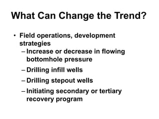
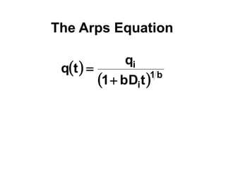
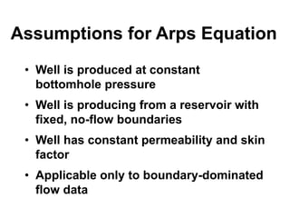
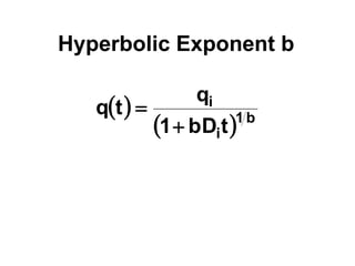
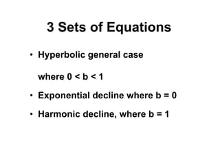
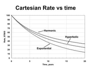
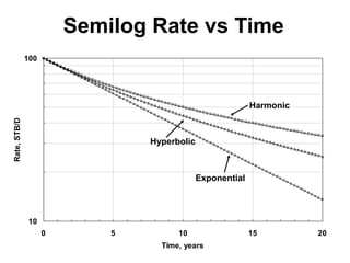
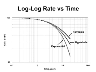
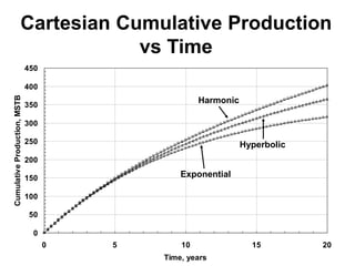
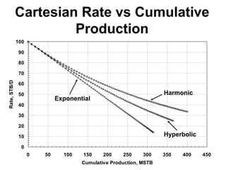
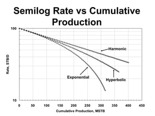
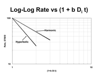
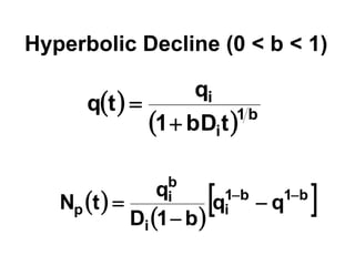
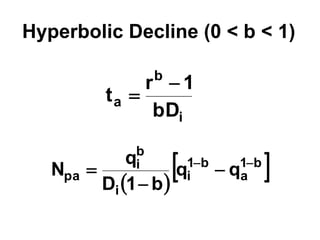
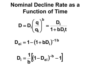
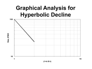
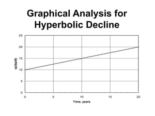
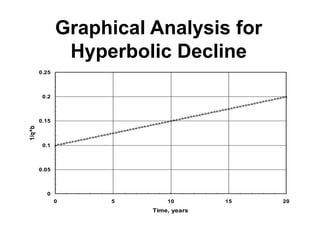
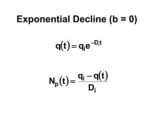
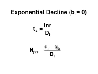
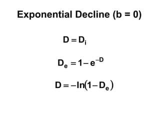
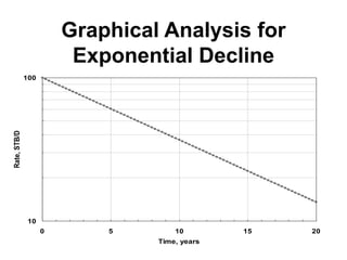
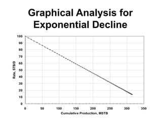
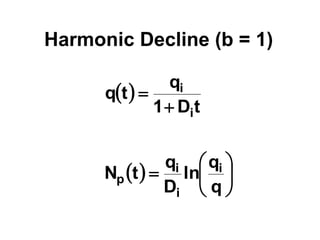
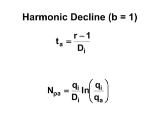
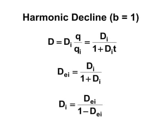
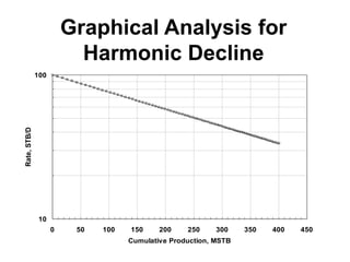
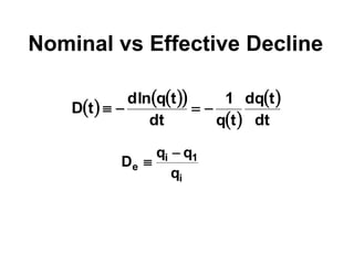
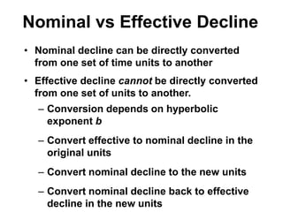
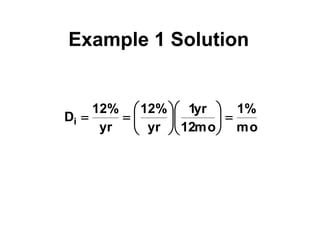
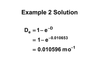
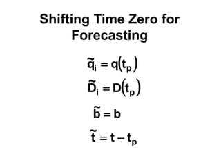
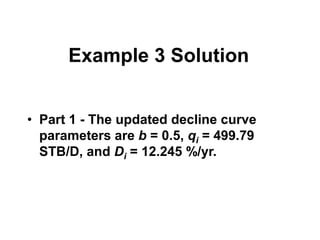
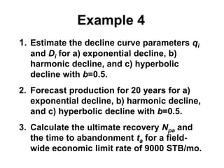
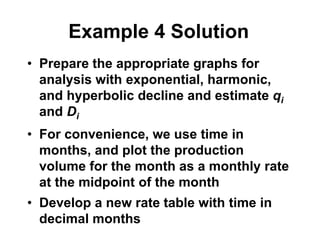
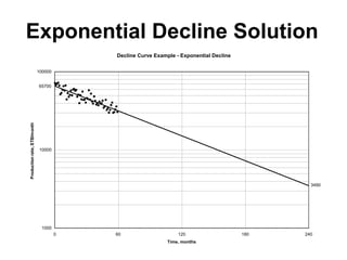
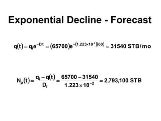
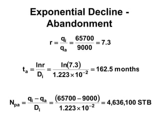
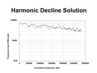
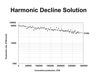
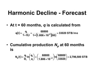
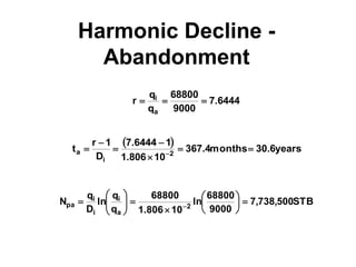
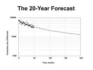
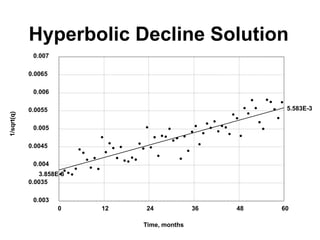
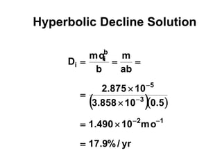
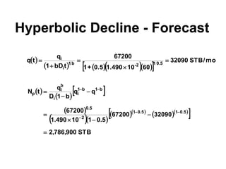
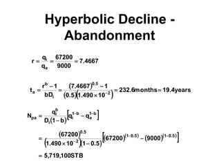
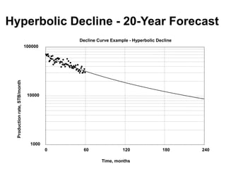
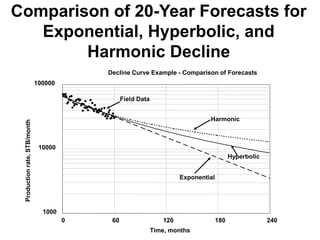
The document outlines the principles and equations of conventional decline curve analysis, emphasizing its importance in matching past performance and forecasting future production. It details various decline models, including exponential, hyperbolic, and harmonic decline, alongside mathematical equations to estimate production and reserve forecasts. Additionally, it addresses the effects of operational changes on decline trends and provides examples for estimating decline parameters and conversion between nominal and effective decline rates.

1. Conventional Decline Curve
Analysis

2. Decline Curve Analysis
Instructional Objectives
• Use conventional decline curve
analysis
• Use effective and nominal decline
equations
• Use exponential and harmonic decline

3. Decline Curve Analysis
Instructional Objectives
• Match past performance
• Forecast future performance

4. Why Do We Use Decline Curve
Analysis?
• Match past performance trends with a
model
– Forecast future
– Estimate reserves

5. What Can Change the Trend?
• Field operations, development
strategies
– Increase or decrease in flowing
bottomhole pressure
– Drilling infill wells
– Drilling stepout wells
– Initiating secondary or tertiary
recovery program

6. The Arps Equation
 
  b
1
i
i
t
bD
1
q
t
q



7. Assumptions for Arps Equation
• Well is produced at constant
bottomhole pressure
• Well is producing from a reservoir with
fixed, no-flow boundaries
• Well has constant permeability and skin
factor
• Applicable only to boundary-dominated
flow data

8. Hyperbolic Exponent b
 
  b
1
i
i
t
bD
1
q
t
q



9. 3 Sets of Equations
• Hyperbolic general case
where 0 < b < 1
• Exponential decline where b = 0
• Harmonic decline, where b = 1

10. 0
10
20
30
40
50
60
70
80
90
100
0 5 10 15 20
Time, years
Rate,
STB/D
Cartesian Rate vs time
Exponential
Hyperbolic
Harmonic

11. 10
100
0 5 10 15 20
Time, years
Rate,
STB/D
Semilog Rate vs Time
Exponential
Hyperbolic
Harmonic

12. 10
100
0.1 1 10 100
Time, years
Rate,
STB/D
Harmonic
Log-Log Rate vs Time
Exponential
Hyperbolic

13. 0
50
100
150
200
250
300
350
400
450
0 5 10 15 20
Time, years
Cumulative
Production,
MSTB
Cartesian Cumulative Production
vs Time
Exponential
Hyperbolic
Harmonic

14. 0
10
20
30
40
50
60
70
80
90
100
0 50 100 150 200 250 300 350 400 450
Cumulative Production, MSTB
Rate,
STB/D
Harmonic
Cartesian Rate vs Cumulative
Production
Exponential
Hyperbolic

15. 10
100
0 50 100 150 200 250 300 350 400 450
Cumulative Production, MSTB
Rate,
STB/D
Semilog Rate vs Cumulative
Production
Exponential
Hyperbolic
Harmonic

16. 10
100
1 10
(1+b Di t)
Rate,
STB/D
Log-Log Rate vs (1 + b Di t)
Hyperbolic
Harmonic

17. Hyperbolic Decline (0 < b < 1)
 
  b
1
i
i
t
bD
1
q
t
q


 
 
 
b
1
b
1
i
i
b
i
p q
q
b
1
D
q
t
N 





18. Hyperbolic Decline (0 < b < 1)
i
b
a
bD
1
r
t


 
 
b
1
a
b
1
i
i
b
i
pa q
q
b
1
D
q
N 





19. Nominal Decline Rate as a
Function of Time
t
bD
1
D
q
q
D
D
i
i
b
i
i











  b
1
i
ei bD
1
1
D 



 
 
1
D
1
b
1
D b
ei
i 

 

20. Graphical Analysis for
Hyperbolic Decline
10
100
1 10
(1+b Di t)
Rate,
STB/D

21. Graphical Analysis for
Hyperbolic Decline
0
5
10
15
20
25
0 5 10 15 20
Time, years
-q/(dq/dt)

22. Graphical Analysis for
Hyperbolic Decline
0
0.05
0.1
0.15
0.2
0.25
0 5 10 15 20
Time, years
1/q^b

23. Exponential Decline (b = 0)
  t
D
i
i
e
q
t
q 

   
i
i
p
D
t
q
q
t
N



24. Exponential Decline (b = 0)
i
a
D
r
ln
t 
i
a
i
pa
D
q
q
N



25. i
D
D 
 
e
D
1
ln
D 


D
e e
1
D 


Exponential Decline (b = 0)

26. Graphical Analysis for
Exponential Decline
10
100
0 5 10 15 20
Time, years
Rate,
STB/D

27. Graphical Analysis for
Exponential Decline
0
10
20
30
40
50
60
70
80
90
100
0 50 100 150 200 250 300 350
Cumulative Production, MSTB
Rate,
STB/D

28. Harmonic Decline (b = 1)
 
t
D
1
q
t
q
i
i


  






q
q
ln
D
q
t
N i
i
i
p

29. i
a
D
1
r
t











a
i
i
i
pa
q
q
ln
D
q
N
Harmonic Decline (b = 1)

30. t
D
1
D
q
q
D
D
i
i
i
i



i
i
ei
D
1
D
D


ei
ei
i
D
1
D
D


Harmonic Decline (b = 1)

31. Graphical Analysis for
Harmonic Decline
10
100
0 50 100 150 200 250 300 350 400 450
Cumulative Production, MSTB
Rate,
STB/D

32. Nominal vs Effective Decline
   
 
 
 
dt
t
dq
t
q
1
dt
t
q
ln
d
t
D 



i
1
i
e
q
q
q
D



33. • Nominal decline can be directly converted
from one set of time units to another
• Effective decline cannot be directly converted
from one set of units to another.
– Conversion depends on hyperbolic
exponent b
– Convert effective to nominal decline in the
original units
– Convert nominal decline to the new units
– Convert nominal decline back to effective
decline in the new units
Nominal vs Effective Decline

34. Example 1
Convert a nominal decline of 12 %/yr to
%/mo

35. Example 1 Solution
mo
%
1
mo
12
yr
1
yr
%
12
yr
%
12
Di 















36. Example 2
• Convert an effective decline rate De =
12%/yr to %/mo, assuming exponential
decline

37. Example 2 Solution
1
010653
.
0
D
e
mo
010596
.
0
e
1
e
1
D









38. Shifting Time Zero for
Forecasting
 
p
i t
q
q
~ 
 
p
i t
D
D
~

b
b
~

p
t
t
t
~



39. Example 3
• Determine the values of qi, Di, and b for
Well X, using the data in your notes and
the current date, 1/1/97, as time zero.

40. Example 3 Solution
• Part 1 - The updated decline curve
parameters are b = 0.5, qi = 499.79
STB/D, and Di = 12.245 %/yr.

41. • Part 2 - The cumulative production from
1/1/97 through 12/30/2000 is 586,152 STB
Example 3 Solution

42. Example 3 Solution
• Part 3 - Cumulative production from
1/1/97 through 12/30/2000:
STB
159
,
586
670413
1256572
Np 



43. Estimating b From Reservoir
Drive Mechanism
• Each drive mechanism has a
characteristic b value
• If b cannot be estimated from
production data, b may be estimated
from the drive mechanism

44. Estimating b from Reservoir
Drive Mechanism
References

45. Example 4
1. Estimate the decline curve parameters qi
and Di for a) exponential decline, b)
harmonic decline, and c) hyperbolic
decline with b=0.5.
2. Forecast production for 20 years for a)
exponential decline, b) harmonic decline,
and c) hyperbolic decline with b=0.5.
3. Calculate the ultimate recovery Npa and
the time to abandonment ta for a field-
wide economic limit rate of 9000 STB/mo.

46. Example 4 Solution
• Prepare the appropriate graphs for
analysis with exponential, harmonic,
and hyperbolic decline and estimate qi
and Di
• For convenience, we use time in
months, and plot the production
volume for the month as a monthly rate
at the midpoint of the month
• Develop a new rate table with time in
decimal months

47. Exponential Decline Solution
Decline Curve Example - Exponential Decline
1000
10000
100000
0 60 120 180 240
Time, months
Production
rate,
STB/month
65700
3490

48. Exponential Decline - Forecast
      
mo
/
STB
31540
e
65700
e
q
t
q 60
10
223
.
1
t
D
i
2
i







   
STB
100
,
793
,
2
10
223
.
1
31540
65700
D
t
q
q
t
N 2
i
i
p 




 

49. Exponential Decline -
Abandonment
3
.
7
9000
65700
q
q
r
a
i



 
months
5
.
162
10
223
.
1
3
.
7
ln
D
r
ln
t 2
i
a 


 
 
STB
100
,
636
,
4
10
223
.
1
9000
65700
D
q
q
N 2
i
a
i
pa 




 

50. Harmonic Decline Solution
• For harmonic decline, we graph q vs Np on
a semilog scale
• First, we have to compute the cumulative
production as a function of time
• Simply adding the monthly volumes will
give the cumulative production at the end
of each month
• Production rate is calculated as an
average over the month, and should be
plotted at the middle of each month

51. Harmonic Decline Solution
• To get cumulative production at the
middle of month j+1, use
 
1
j
j
2
1
j
p
1
j
j
p
2
1
j
p q
q
5
.
0
N
q
5
.
0
N
N 


 





52. Harmonic Decline Solution

53. Harmonic Decline Solution
1000
10000
100000
0 500000 1000000 1500000 2000000 2500000 3000000
Cumulative production, STB
Production
rate,
STB/month

54. Harmonic Decline Solution
0 500000 1000000 1500000 2000000 2500000 3000000
Cumulative production, STB
Production
rate,
STB/month
1000
10000
100000
68800
31300

55. Harmonic Decline - Forecast
• At t = 60 months, q is calculated from
• Cumulative production Np at 60 months
is
  STB
500
,
796
,
2
33020
68800
ln
10
806
.
1
68800
q
q
ln
D
q
t
N 2
i
i
i
p 




















 
 
  
mo
/
STB
33020
60
10
1.806
+
1
68800
t
D
1
q
t
q 2
-
i
i






56. Harmonic Decline -
Abandonment
6444
.
7
9000
68800
q
q
r
a
i



 
years
6
.
30
months
4
.
367
10
806
.
1
1
6444
.
7
D
1
r
t 2
i
a 





 
STB
500
,
738
,
7
9000
68800
ln
10
806
.
1
68800
q
q
ln
D
q
N 2
a
i
i
i
pa 
















 

57. The 20-Year Forecast
1000
10000
100000
0 60 120 180 240
Time, months
Production
rate,
STB/month

58. Hyperbolic Decline Solution
0.003
0.0035
0.004
0.0045
0.005
0.0055
0.006
0.0065
0.007
0 12 24 36 48 60
Time, months
1/sqrt(q)
3.858E-3
5.583E-3

59.   
yr
/
%
9
.
17
mo
10
490
.
1
5
.
0
10
858
.
3
10
875
.
2
ab
m
b
mq
D
1
2
3
5
b
i
i













Hyperbolic Decline Solution

60. Hyperbolic Decline - Forecast
 
     
 
mo
/
STB
32090
60
10
1.490
0.5
+
1
67200
t
bD
1
q
t
q 5
.
0
1
2
-
b
1
i
i





 
 
 
 
  
  
  
 
STB
900
,
786
,
2
32090
67200
5
.
0
1
10
490
.
1
67200
q
q
b
1
D
q
t
N
5
.
0
1
5
.
0
1
2
5
.
0
b
1
b
1
i
i
b
i
p














61. Hyperbolic Decline -
Abandonment
4667
.
7
9000
67200
q
q
r
a
i



 
   years
4
.
19
months
6
.
232
10
490
.
1
5
.
0
1
4667
.
7
bD
1
r
t 2
5
.
0
i
b
a 





 
 
 
 
  
  
  
 
STB
100
,
719
,
5
9000
67200
5
.
0
1
10
490
.
1
67200
q
q
b
1
D
q
N
5
.
0
1
5
.
0
1
2
5
.
0
b
1
a
b
1
i
i
b
i
pa














62. Hyperbolic Decline - 20-Year Forecast
Decline Curve Example - Hyperbolic Decline
1000
10000
100000
0 60 120 180 240
Time, months
Production
rate,
STB/month

63. Comparison of 20-Year Forecasts for
Exponential, Hyperbolic, and
Harmonic Decline
Decline Curve Example - Comparison of Forecasts
1000
10000
100000
0 60 120 180 240
Time, months
Production
rate,
STB/month
Field Data
Exponential
Hyperbolic
Harmonic