This document discusses decline curve analysis for predicting the depletion of natural resources like oil. It presents Hubbert's peak theory, which models the production rate of a resource over time as demand increases and peaks before dropping off. The objective of decline curve analysis is to predict production declines based on past data by fitting curves like exponential, harmonic, or hyperbolic models. Different curve types can model production declines for individual wells, fields, or groups of fields.

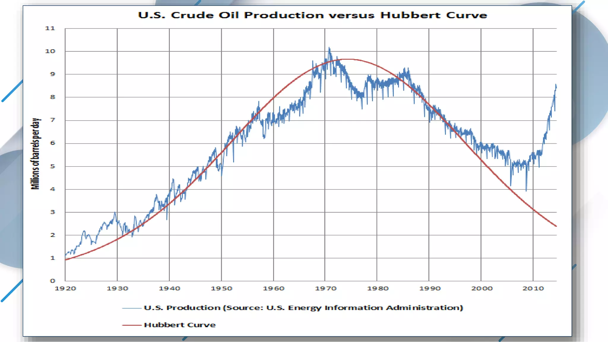
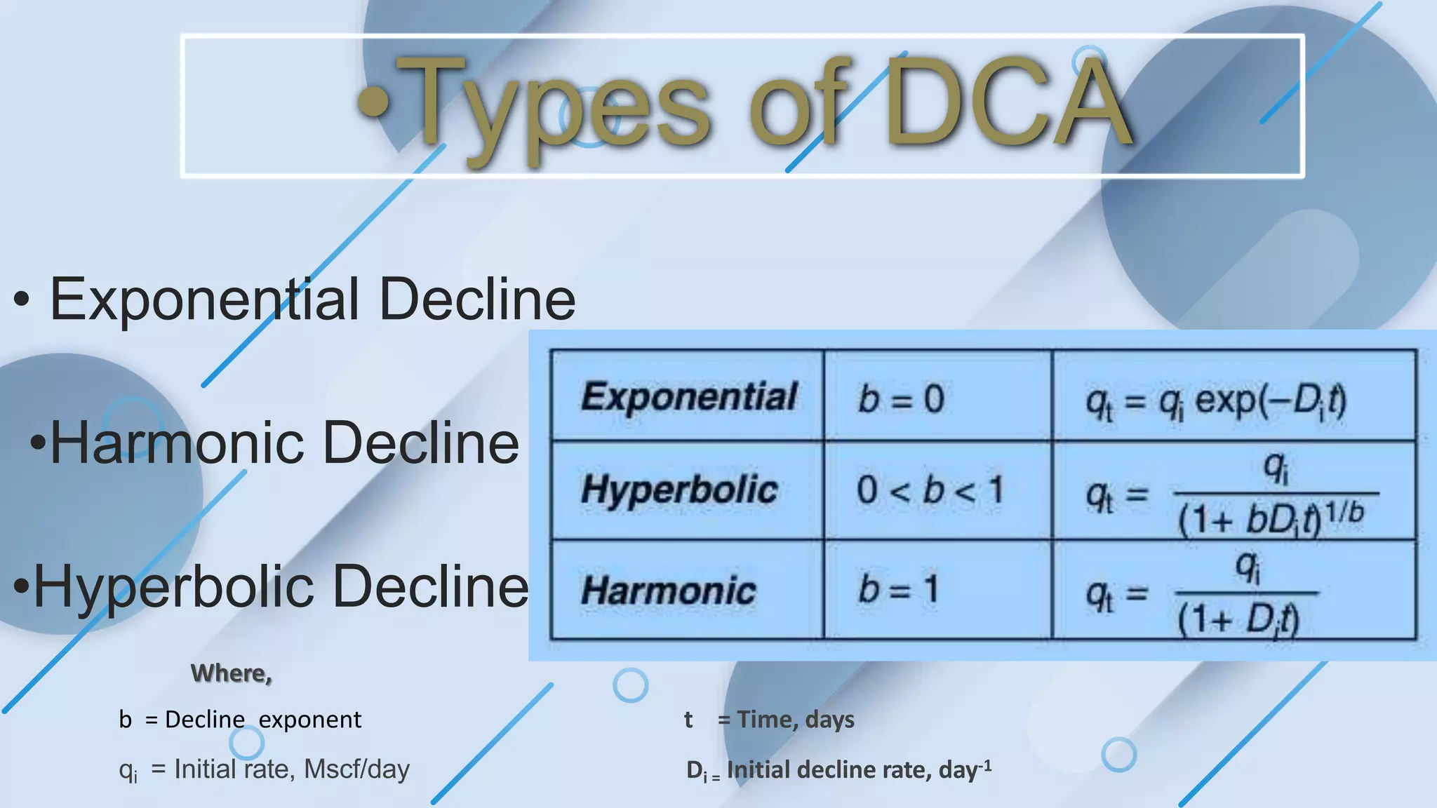
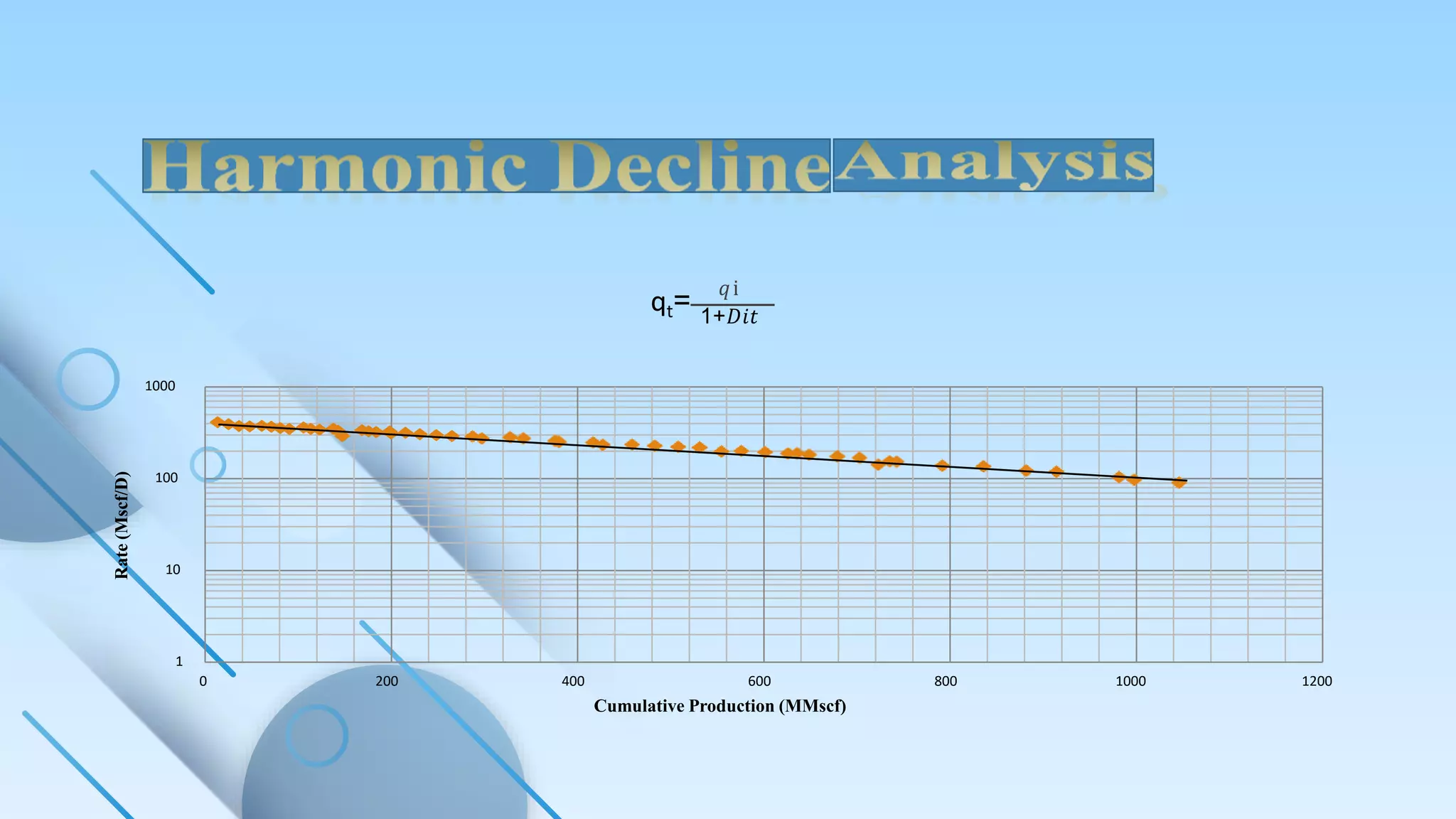
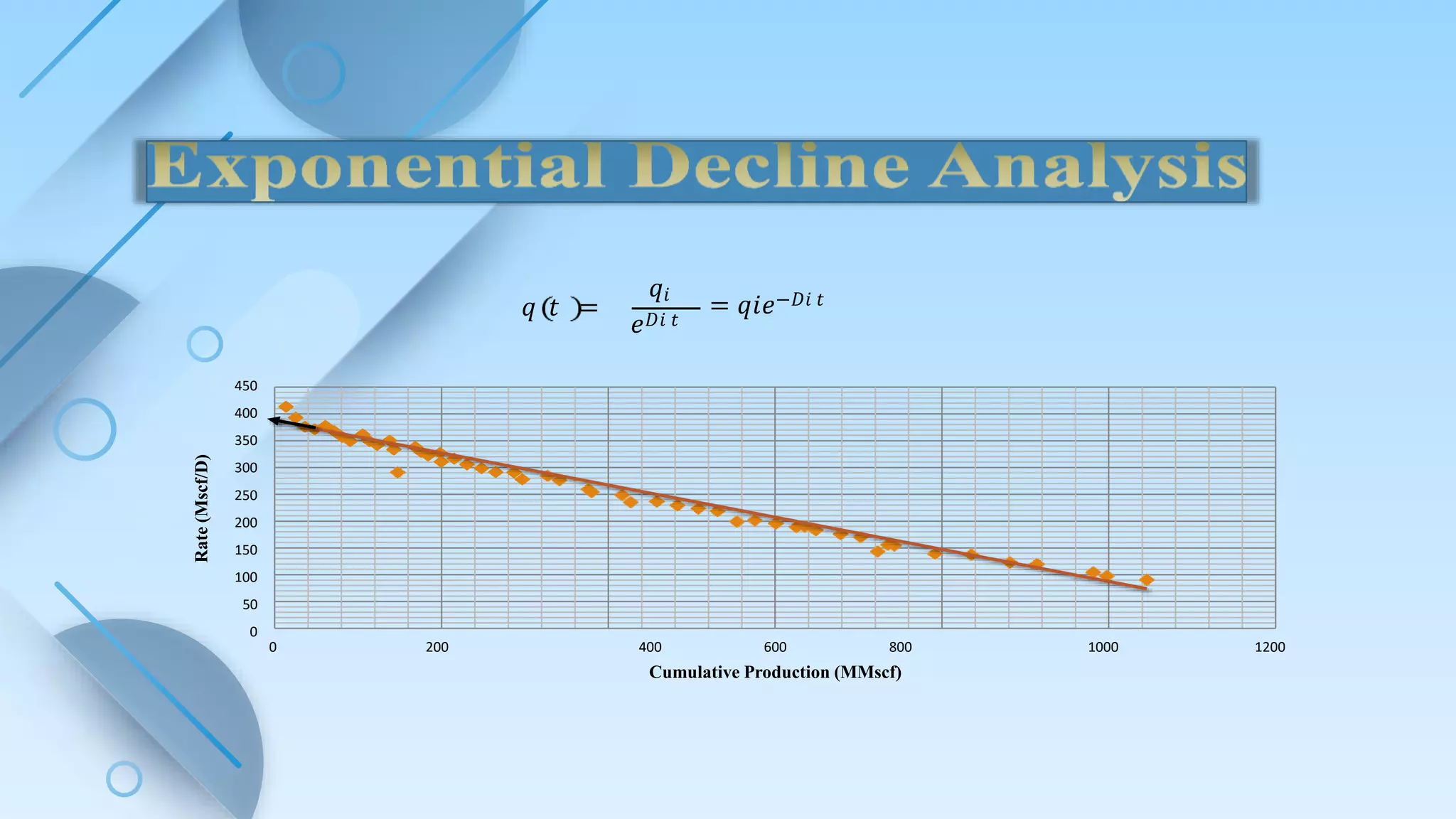
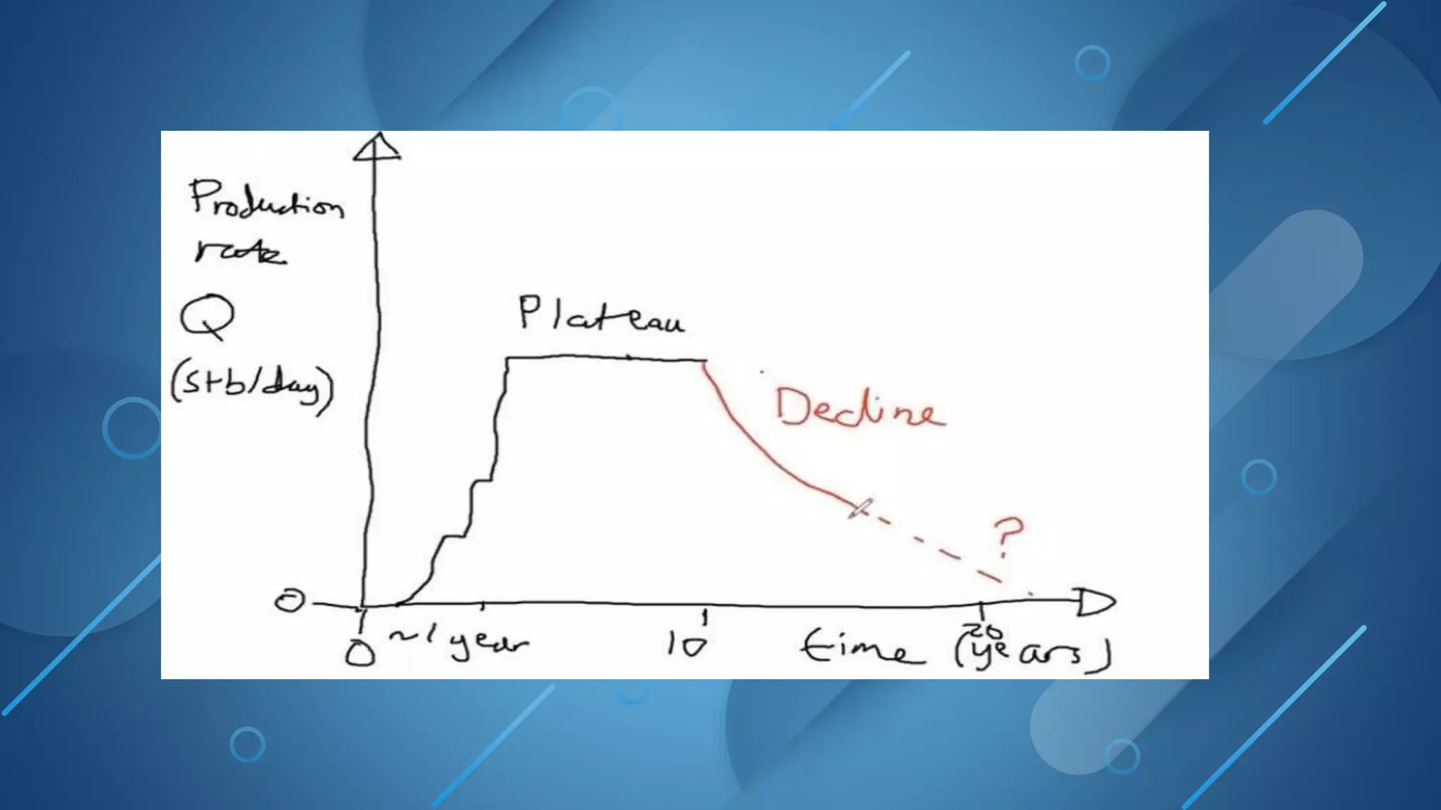
1. By:
Mohammed Alghanoudi
Supervised by:
Dr. Ibrahim
Sabratha Faculty of Engineering
Petroleum engineering department
Drilling fluids laboratory
Decline Curve Analysis

2. Contents Introduction
01
Objective
02
Hubbert's theory
03
Chart
04

3. INTRODUCTION
 In the short and medium term, declines in oil production occur in
a predictable manner based on geological conditions,
government policies, and engineering practices. The shape of
the slope curve varies depending on whether one is considering
a well, a field, or a group of fields. In the long term, technological
developments have challenged some of these expectations.
 The decline curve analysis technique relies on analyzing the
previous data for the decline in production performance, which is
expressed in charts that link the production rate and time, or the
production rate and cumulative productivity. And that's for
everyone. wells And Reservoirs.

4. OBJECTIVE
To predict the depletion of various natural
resources.
The aim of this analysis is to:

5. Hubbert's theory
 Hubbert's peak or Hubbert's curve is a model that approximates the
production rate of a resource over a period of time. Specifically, Hubbert's
peak refers to the point at which this production rate is at its highest with
demand for the resource rising, and after this it predicts a drop in
correlation to the increased demand.
 During this drop, there may be dramatic differences in production and
demand as demand continues to increase but production drops overall.
 Figure 1 shows Hubbert's predicted model compared to US oil production.
Although this model can be applied to many resources, it was initially
developed as a model for oil production.

7. •Types of DCA
• Exponential Decline
•Harmonic Decline
•Hyperbolic Decline
Where,
b = Decline exponent
qi = Initial rate, Mscf/day
t = Time, days
Di = Initial decline rate, day-1

8. 𝑞i
qt= 1+𝐷𝑖𝑡
1
10
100
1000
0 200 400 600 800 1000 1200
Rate
(Mscf/D)
Cumulative Production (MMscf)

9. 450
400
350
300
250
200
150
100
50
0
0 200 400 600 800
Cumulative Production (MMscf)
1000 1200
Rate
(Mscf/D)
𝑞 𝑡 =
𝑞𝑖
𝑒𝐷𝑖 𝑡
= 𝑞𝑖𝑒−𝐷𝑖 𝑡

11. References:
 M. King Hubbert. " (PDF). Drilling and Production Practice (1956)
American Petroleum Institute & Shell Development Co. Publication No. 95, See Pp 9-11, 21-
22. Archived from (PDF) on 2008-05-27.^
 Ugo Bardi and Leigh Yaxley. ] Proceedings of the 4th Workshop, Lisbon 2005^ Jean
Laherrere. . July, 1997.^ Patzek, Tad (2008-05-17).
 " ". Archives
of Mining Sciences. 53 (2): 131–159. Retrieved 2018-11-17.

12. THANK YOU FOR LISTENING