This document summarizes an experimental investigation into the thermal behavior of steam turbine components during natural cooling. Key points:
- Optical probes and thermocouples were used to measure the temperature of a steam turbine rotor and casings over 96 hours of natural cooling after shutdown.
- A 2D numerical model was developed to simulate the natural cooling process by replacing fluid buoyancy with an equivalent fluid conductivity based on experimental data.
- Measurements found the rotor and some casing locations initially increased in temperature after active cooling ended, then cooled over time.
- The results provide data to optimize steam turbines for flexible operation by better understanding how initial metal temperatures affect startup stresses and fatigue life.
![Gabriel Marinescu
e-mail: gabriel.marinescu@power.alstom.com
Wolfgang F. Mohr
e-mail: wolfgang.mohr@power.alstom.com
Andreas Ehrsam
e-mail: andreas.ehrsam@power.alstom.com
Paolo Ruffino
e-mail: paolo.ruffiono@power.alstom.com
Michael Sell
e-mail: michael.sell@power.alstom.com
Alstom, Power
Baden 5401, Switzerland
Experimental Investigation Into
Thermal Behavior of Steam
Turbine Components—
Temperature Measurements
With Optical Probes and Natural
Cooling Analysis
The steam turbine cooldown has a significant impact on the cyclic fatigue life. A lower ini-
tial metal temperature after standstill results in a higher temperature difference to be over-
come during the next start-up. Generally, lower initial metal temperatures result in higher
start-up stress. In order to optimize steam turbines for cyclic operation, it is essential to
fully understand natural cooling, which is especially challenging for rotors. This paper
presents a first-in-time application of a 2D numerical procedure for the assessment of the
thermal regime during natural cooling, including the rotors, casings, valves, and main
pipes. The concept of the cooling calculation is to replace the fluid gross buoyancy during
natural cooling by an equivalent fluid conductivity that gives the same thermal effect on
the metal parts. The fluid equivalent conductivity is calculated based on experimental data.
The turbine temperature was measured with pyrometric probes on the rotor and with
standard thermocouples on inner and outer casings. The pyrometric probes were cali-
brated with standard temperature measurements on a thermo well, where the steam trans-
mittance and the rotor metal transmissivity were measured. [DOI: 10.1115/1.4025556]
Introduction
Modern steam turbines are operated at high pressure and tem-
perature. In addition many steam power plants are today subject
to operation modes such as double shifts or load following opera-
tion. Especially for combined cycle power plants and solar ther-
mal plants fast start-up and high operational flexibility is required.
At base load operation the hot components are exposed to
creep. Additionally, high fatigue occurs because of the thermal
stress during transient events such as start-up, shut down, or load
changes. In order to design a fast starting and flexible steam tur-
bine, the engineer deals with an important challenge due to the
sensitivity of the cyclic lifetime assessment. The thermal stress
arising in the hot thick-walled turbine components such as rotor,
valves, and casings during turbine start-up is directly related to
the temperature gradient. The highest stress occurs when the
machine ramps up from standstill to base load condition. For an
accurate thermal stress calculation the temperature profile
becomes a very important parameter. This paper presents a
method for the assessment of the thermal regime during natural
cooling of steam turbines.
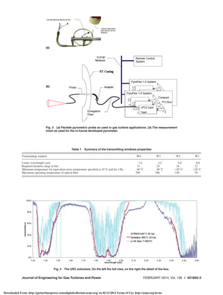
Instrumentation With Optical Probes
An operational Alstom KA26-1 unit was instrumented with
three optical probes OT1, OT2, OT3; with 24 thermocouples type
N class A on inner casing; and with 40 thermocouples type N
class A metal sheet protected on outer casing as presented on
Fig. 1. This was the first field turbine instrumented
with optical pyrometers tracking the rotor temperature for almost
96 h. The inner casing during instrumentation at the Alstom
Morelia—Mexico plant is presented on Fig. 2.
Alstom has developed in-house a flexible, fiber-based pyrome-
ter [1–3] shown on Fig. 3. The flexible pyrometer consists of a
probe containing a low-OH gold-coated high temperature optical
glass fiber with a diameter of 0.3 mm and a numerical aperture of
0.2. At the tip of the probe there is a sapphire lens of Ø2.4 mm,
which reduces the numerical aperture of the system to 0.04. The
signal picked up by the probe is then sent to an optical detector,
an InGaAs PIN photodiode (three layer photo-diode with an
intrinsec layer between the p- and n-type regions), G5853 of
Hamamatsu. The photodiode is directly mounted to a compact pe-
ripheral component interconnect card, which is based on a Motor-
ola DSP56000 digital signal processor. The signal processor reads
the data of a 24 bit analog to digital converter with a sampling rate
of 100,000 per second and converts the measured intensity
directly into temperature. At temperatures above 230
C, the tem-
perature precision of the optical probe is better than 61.5
C [1].
Below this temperature, the precision quickly deteriorates and at
150
C reaches 610
C. Below 130
C the signal is useless as long
as the irradiation signal vanishes in the dark current of the
photodiode.
Literature about the transmissivity of high-pressure stream is
very limited. Available papers and calculations are based on low-
pressure data sets. This data highlights several transmitting
windows between strong absorption bands of steam, which are
determined by the rotational and vibrational quantum states. The
lowest window W1 is located between 8 and 12 lm. At longer
wavelengths the light is absorbed by pure rotational transitions,
while at shorter wavelengths the light is absorbed by a rovibra-
tional transition of the symmetric bend. The next windows range
from 3.5 to 4.3 lm (W2), from 2.0 to 2.4 lm (W3), and from 1.5
to 1.7 lm (W4) (see Table 1).
Further, even more narrow consecutive windows exist toward
shorter wavelengths. However, the blackbody radiation density
Contributed by the Controls, Diagnostics and Instrumentation Committee of
ASME for publication in the JOURNAL OF ENGINEERING FOR GAS TURBINES AND POWER.
Manuscript received August 31, 2013; final manuscript received September 10,
2013; published online November 1, 2013. Editor: David Wisler.
Journal of Engineering for Gas Turbines and Power FEBRUARY 2014, Vol. 136 / 021602-1
Copyright VC 2014 by ASME
Downloaded From: http://gasturbinespower.asmedigitalcollection.asme.org/ on 02/12/2014 Terms of Use: http://asme.org/terms](https://image.slidesharecdn.com/ad137663-a8d7-4099-8b83-dc228dbb5cb9-160320075113/85/01-GTP-13-1334-1-320.jpg)
![Gabriel Marinescu
e-mail: gabriel.marinescu@power.alstom.com
Wolfgang F. Mohr
e-mail: wolfgang.mohr@power.alstom.com
Andreas Ehrsam
e-mail: andreas.ehrsam@power.alstom.com
Paolo Ruffino
e-mail: paolo.ruffiono@power.alstom.com
Michael Sell
e-mail: michael.sell@power.alstom.com
Alstom, Power
Baden 5401, Switzerland
Experimental Investigation Into
Thermal Behavior of Steam
Turbine Components—
Temperature Measurements
With Optical Probes and Natural
Cooling Analysis
The steam turbine cooldown has a significant impact on the cyclic fatigue life. A lower ini-
tial metal temperature after standstill results in a higher temperature difference to be over-
come during the next start-up. Generally, lower initial metal temperatures result in higher
start-up stress. In order to optimize steam turbines for cyclic operation, it is essential to
fully understand natural cooling, which is especially challenging for rotors. This paper
presents a first-in-time application of a 2D numerical procedure for the assessment of the
thermal regime during natural cooling, including the rotors, casings, valves, and main
pipes. The concept of the cooling calculation is to replace the fluid gross buoyancy during
natural cooling by an equivalent fluid conductivity that gives the same thermal effect on
the metal parts. The fluid equivalent conductivity is calculated based on experimental data.
The turbine temperature was measured with pyrometric probes on the rotor and with
standard thermocouples on inner and outer casings. The pyrometric probes were cali-
brated with standard temperature measurements on a thermo well, where the steam trans-
mittance and the rotor metal transmissivity were measured. [DOI: 10.1115/1.4025556]
Introduction
Modern steam turbines are operated at high pressure and tem-
perature. In addition many steam power plants are today subject
to operation modes such as double shifts or load following opera-
tion. Especially for combined cycle power plants and solar ther-
mal plants fast start-up and high operational flexibility is required.
At base load operation the hot components are exposed to
creep. Additionally, high fatigue occurs because of the thermal
stress during transient events such as start-up, shut down, or load
changes. In order to design a fast starting and flexible steam tur-
bine, the engineer deals with an important challenge due to the
sensitivity of the cyclic lifetime assessment. The thermal stress
arising in the hot thick-walled turbine components such as rotor,
valves, and casings during turbine start-up is directly related to
the temperature gradient. The highest stress occurs when the
machine ramps up from standstill to base load condition. For an
accurate thermal stress calculation the temperature profile
becomes a very important parameter. This paper presents a
method for the assessment of the thermal regime during natural
cooling of steam turbines.
Instrumentation With Optical Probes
An operational Alstom KA26-1 unit was instrumented with
three optical probes OT1, OT2, OT3; with 24 thermocouples type
N class A on inner casing; and with 40 thermocouples type N
class A metal sheet protected on outer casing as presented on
Fig. 1. This was the first field turbine instrumented
with optical pyrometers tracking the rotor temperature for almost
96 h. The inner casing during instrumentation at the Alstom
Morelia—Mexico plant is presented on Fig. 2.
Alstom has developed in-house a flexible, fiber-based pyrome-
ter [1–3] shown on Fig. 3. The flexible pyrometer consists of a
probe containing a low-OH gold-coated high temperature optical
glass fiber with a diameter of 0.3 mm and a numerical aperture of
0.2. At the tip of the probe there is a sapphire lens of Ø2.4 mm,
which reduces the numerical aperture of the system to 0.04. The
signal picked up by the probe is then sent to an optical detector,
an InGaAs PIN photodiode (three layer photo-diode with an
intrinsec layer between the p- and n-type regions), G5853 of
Hamamatsu. The photodiode is directly mounted to a compact pe-
ripheral component interconnect card, which is based on a Motor-
ola DSP56000 digital signal processor. The signal processor reads
the data of a 24 bit analog to digital converter with a sampling rate
of 100,000 per second and converts the measured intensity
directly into temperature. At temperatures above 230
C, the tem-
perature precision of the optical probe is better than 61.5
C [1].
Below this temperature, the precision quickly deteriorates and at
150
C reaches 610
C. Below 130
C the signal is useless as long
as the irradiation signal vanishes in the dark current of the
photodiode.
Literature about the transmissivity of high-pressure stream is
very limited. Available papers and calculations are based on low-
pressure data sets. This data highlights several transmitting
windows between strong absorption bands of steam, which are
determined by the rotational and vibrational quantum states. The
lowest window W1 is located between 8 and 12 lm. At longer
wavelengths the light is absorbed by pure rotational transitions,
while at shorter wavelengths the light is absorbed by a rovibra-
tional transition of the symmetric bend. The next windows range
from 3.5 to 4.3 lm (W2), from 2.0 to 2.4 lm (W3), and from 1.5
to 1.7 lm (W4) (see Table 1).
Further, even more narrow consecutive windows exist toward
shorter wavelengths. However, the blackbody radiation density
Contributed by the Controls, Diagnostics and Instrumentation Committee of
ASME for publication in the JOURNAL OF ENGINEERING FOR GAS TURBINES AND POWER.
Manuscript received August 31, 2013; final manuscript received September 10,
2013; published online November 1, 2013. Editor: David Wisler.
Journal of Engineering for Gas Turbines and Power FEBRUARY 2014, Vol. 136 / 021602-1
Copyright VC 2014 by ASME
Downloaded From: http://gasturbinespower.asmedigitalcollection.asme.org/ on 02/12/2014 Terms of Use: http://asme.org/terms](https://image.slidesharecdn.com/ad137663-a8d7-4099-8b83-dc228dbb5cb9-160320075113/75/01-GTP-13-1334-1-2048.jpg)
![below 1.5 lm is too small to be used for high precision tempera-
ture determination in the range from 250
C up to 700
C.
The steam transmittance is crucial for the intensity pyrometry
in steam turbines. The usual approach [4] is to extrapolate the
pressure broadening measured on low-pressure measurements as
shown in Refs. [5–7]. This is dangerous, as low-pressure broaden-
ing effects are dominated by two-body interactions, whereas high-
pressure broadening effects are affected by many-body interac-
tions or even spectral shifts caused by water clusters. Such many-
body effects reduce the lifetime of the molecular rovibrational
levels, which further increases the pressure broadening. Also to be
considered are line shape effects caused by the slow falloff of the
Lorenzian, Dicke [8], and Galatry [9] type. The slow falloff of
these lines shapes leads at high pressure to a long-range artifact,
where far from any line, like at 2.5 lm, the residual absorption
may reach significant levels.
Measurements at high pressure are rare. We found absorption
cell measurements [10,11] and shock-tube results [12] discussing
the line shape but no measurements in the transmitting windows.
Therefore, a dedicated autoclave was designed (see Fig. 4). The
steam measured transmittance at 30bar and 600
C is shown on
Fig. 5 in comparison to extrapolated low resolution measurements
from Goldstein [10]. The program Spectralcalc was used to calcu-
late the spectra. This program uses the line assignments of the
HITRAN and HITEMP [13] database to calculate the strengths of
the lines as function of the temperature and uses the low-pressure
broadening data to linearly extrapolate the transmittance spectra to
very high pressures. The comparison between the theoretical pre-
diction and the featured wavelengths shows good agreement. The
results of the transmittance tests indicated that the intensity pyrome-
try for IP and in particular for HP steam turbines is best conducted
in the steam transmittance window W4 at wavelength 1.6 lm.
The optical probe lenses were protected against FeO particles
contamination with a nitrogen purge device. Figure 6 shows a
comparison between a contaminated and purged lens in a real
steam turbine. This comparison confirmed that the purge was
mandatory to ensure measurement accuracy.
Measured Temperatures
The natural cooling measurements were conducted in Decem-
ber 2010 during the power-plant commissioning phase. The
machine consists of a GT26 gas turbine and a HP-IP-LP steam tur-
bine. Before starting the natural cooling measurements the
machine was stabilized at base load regime. From base load the
steam turbine was by-passed and disconnected from the gas
turbine. The glands system was maintained active together with
vacuum in the turbine cavity for 3 h 15 min. After that the glands
system was deactivated and ambient pressure established within
the turbine cavity. The thermocouples and optical probe signals
recorded the metal temperature for 96 h. After 96 h the machine
was ramped up to base load regime.
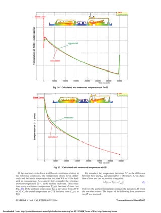
Figure 7 shows the transient temperatures measured by the opti-
cal probes OT1, OT2, and OT3. The temperatures are given in
nondimensional format, divided by the live steam temperature at
base load. The temperatures where this ratio is below 0.35 reached
the accuracy limit of the pyrometric method and were
disregarded.
Some of the temperatures recorded at the thermocouples loca-
tion are presented on Fig. 8.
It must be noted that there are locations both on the inner and
outer casing where the temperature increased within the first hours
after natural cooling start. This phenomenon occurs on the cold
domains once the active cooling specific for base load regime ends.
The Finite Element Analysis
The main difficulty of the natural cooling analysis consists of
the long physical cooling time (approximately 100 h) relative to
the short integration time step (0.01 ms, typically) of the numerical
scheme required for a convergent process. For this reason much
Fig. 2 The IP steam turbine arrangement
Fig. 1 IP steam turbine instrumentation
021602-2 / Vol. 136, FEBRUARY 2014 Transactions of the ASME
Downloaded From: http://gasturbinespower.asmedigitalcollection.asme.org/ on 02/12/2014 Terms of Use: http://asme.org/terms](https://image.slidesharecdn.com/ad137663-a8d7-4099-8b83-dc228dbb5cb9-160320075113/85/01-GTP-13-1334-2-320.jpg)
![attention was paid to the software used for modeling. Ideally the
software has to fulfill the following two conditions: (a) it has to be
able to model the steam ingestion phase when the steam enthalpy
feeding the glands is distributed in the turbine cavity, and (b) it has
to be able to capture the thermal effect of the steam flow in the tur-
bine cavity to transfer the heat from the hot rotor and inner casing
to the outer casing, valves, pipes, and forward to ambient. One of
the finite element applications qualified for these conditions is
SC03, a Rolls-Royce in-house finite element software. Alstom
Power and Rolls-Royce built a SC03 plug in for steam applications
that calculates automatically the steam thermodynamic properties
and the corresponding heat transfer coefficients.
Consequently, a 2D transient SC03 model was built based on
the IP turbine geometry. The steam ingestion during the first 3 h
15 min was modeled adding an assumed shape of the steam jet
contour. Figure 9 shows the jet contour and the location of the
thermocouples T11.1, T24.1, and Tm33. The steam enthalpy was
gradually distributed from A to B along and inside the jet contour.
The numerical experiments showed that the position of the
steam jet contour in the turbine cavity has a negligible impact on
the metal temperature distribution. The most important is to bring
the steam glands energy in the turbine cavity distributed in time in
line with the physical process, which is properly captured in the fi-
nite element model. Condition (b) mentioned above was satisfied
introducing finite elements in the turbine cavity defined with fluid
conductivity (see Fig. 10).
The steam buoyancy, very active during the steam ingestion
phase, can be interpreted as a heat wave that travels in the turbine
cavity, driven by the local thermal gradient. The thermal effect of
this buoyancy can be captured as a temperature-dependent con-
ductivity, higher than a given reference fluid conductivity. As
most of the time the natural cooling phase in the turbine cavity is
air, we considered the air as the reference fluid. The thermal effect
of the local buoyancy was captured via a correction factor K(T)
introduced in the fluid conductivity k(T) [14]. Then, the fluid con-
ductivity in the turbine cavity is
Fig. 6 Effect of purging on the lenses contamination in a real steam turbine (left not purged,
right purged)
Fig. 5 The steam transmittance at 20 bar and 600
C. The calculated curve using the HITRAN
database [13], the low resolution data of Goldstein [10], and our experimental results from the
FTIR spectrometer.
021602-4 / Vol. 136, FEBRUARY 2014 Transactions of the ASME
Downloaded From: http://gasturbinespower.asmedigitalcollection.asme.org/ on 02/12/2014 Terms of Use: http://asme.org/terms](https://image.slidesharecdn.com/ad137663-a8d7-4099-8b83-dc228dbb5cb9-160320075113/85/01-GTP-13-1334-4-320.jpg)
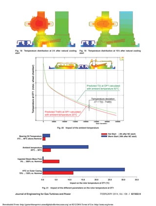
![• bearing oil temperature ¼ nominal temp þ (0
C…40
C)
• ambient temperature ¼ 20
C…50
C
• ingested steam mass flow during the ingestion phase ¼ 0%…
300% relative to the nominal ingested mass flow
• HTC on the outer face of the outer casing ¼ 70%…130%
relative to nominal HTC
Figure 21 collects the temperature deviation DT at OT1 for
each of the above parameters taken at 8 h (hot start condition),
respectively, 60 h (warm start condition) after natural cooling
start.
Figure 21 suggests the following conclusions:
• The deviation of the bearing oil temperature relative to the
standard oil temperature has a low impact (1 deg…3
C) on
rotor temperature at WS and negligible at HS.
• The ambient temperature has a low impact (2 deg…3
C) at
HS and 16 deg…18
C impact at WS.
• The deviation due to the steam ingestion has a 6 deg… 8
C
impact at HS and negligible at WS. The impact of the gland
steam temperature on rotor and casings was assessed in
Ref. [15] Sec. 5.3 and similar conclusions were found.
• The deviation of the thermal insulation quality has
10 deg…12
C impact at HS and a 30
C…32
C impact at
the WS.
Conclusions
A new numerical procedure for the assessment of the thermal
regime during natural cooling of the main steam turbine compo-
nents was validated with experimental measurements. Metal tem-
peratures were measured on the rotor surface of a commercial
steam turbine with in-house developed pyrometers. Additionally a
large number of standard thermocouples were installed on the
inner and outer casing.
The concept of the numerical cooling calculation is to replace
the fluid gross buoyancy during natural cooling by an equivalent
fluid overconductivity that gives the same thermal effect on the
metal parts. This fluid overconductivity function was established
based on experimental data.
The validation proved that the numerical model is able to pre-
dict the cooling of all main steam turbine components with good
accuracy. Based on the large number of metal temperature meas-
urements available, the overall turbine cooling model was vali-
dated. It was demonstrated that the numerical procedure is able to
model the natural cooling heat transfer mechanism for 96 h physi-
cal time on turbine rotor, casings, and valves. The calculation
method, whose accuracy ranges within 0 deg…15
C relative to
measured data, was used to assess the impact of the physical pa-
rameters the ambient air temperature, the steam ingestion time,
the characteristics of thermal insulation, and the bearing oil tem-
perature on the turbine rotor thermal regime.
The numerical cooling model can be used to provide important
information about the thermal state of the turbine parts during var-
ious cooling events such as night shutdown, weekend shutdown,
forced cooling events, etc. This is an important basis for the
design of flexible steam turbines, ready for fast and reliable cyclic
operation.
Nomenclature
a1, a2, a3 ¼ calibration parameters
CCPP ¼ combined cycle power plant
HP ¼ high pressure
HS ¼ hot start
HTC ¼ heat transfer coefficient
IP ¼ intermediate pressure
K(T) ¼ correction factor for fluid conductivity
p ¼ iteration number
T ¼ calculated metal temperature at a thermocouple
location
Tfluid ¼ fluid temperature
Tmeas ¼ measured metal temperature at a thermocouple
location
WS ¼ warm start
k ¼ fluid thermal conductivity
References
[1] Ruffino, P., and Mohr, W., 2012, “Experimental Investigation Into Thermal
Behavior of Steam Turbine Components: Part 1—Temperature Measurements
With Optical Probes,” ASME Paper No. GT2012-68703.
[2] Dobler, T., Haffner, K., and Evers Wolfgang, 1998, “Optic Pyrometer for Gas
Turbines,” U. S, Patent No. 6,109,783.
[3] Kempe, A., Schlamp, S., R€osgen, T., and Haffner, K., 2006, “Optical
Tip-Clearance Probe for Harsh Environments,” The XVIII Symposium on Meas-
uring Techniques in Turbomachinery, Thessaloniki, Greece, September 21–22.
[4] Kirby, P. J., Zachary, R. E., and Ruiz, F., 1986, “Infrared Thermometry for Con-
trol and Monitoring of Industrial Gas Turbines,” ASME Paper No. 86-GT-267.
[5] Phelan, R., Lynch, M., Donegan, J. F., and Weldon, V., 2003, “Absorption Line
Shift With Temperature and Pressure Impact on Laser-Diode-Based H2O Sens-
ing at 1.393 lm,” Appl. Opt., 42, pp. 4968–4974.
[6] Smith, K. M., Ptashnik, I., Newnham, D. A., and Shine, K. P., 2004,
“Absorption by Water Vapour in the 1 to 2 lm Region,” J. Quant. Spec. Radiat.
Transfer, 83, pp. 735–749.
[7] Rothman, L. S., Jacquemart, D., Barbe, A., Chris Benner, D., Birk, M., Brown, L.
R., Carleer, M. R., Chackerian, Jr. C., Chance, K., Coudert, L. H., Dana, V.,
Devi, V. M., Flaud, J.-M., Gamache, R. R., Goldman, A., Hartmann, J.-M., Jucks,
K. W., Maki, A. G., Mandin, J.-Y., Massie, S. T., Orphal, J., Perrin, A., Rinsland,
C. P., Smith, M. A. H., Tennyson, J., Tolchenov, R. N., Toth, R. A., Vander
Auwera, J., Varanasi, P., and Wagner, G., 2005, “The HITRAN 2004 Molecular
Spectroscopic Database,” J. Quant. Spectrosc. Radiat. Transfer, 96, pp. 139–204.
[8] Dicke, R. H., 1953, “The Effect of Collisions Upon the Doppler Width of Spec-
tral Lines,” Phys. Rev., 89, pp. 472–473.
[9] Galatry, L., 1961, “Simultaneous Effect of Doppler and Foreign Gas Broaden-
ing of Spectral Lines,” Phys. Rev., 122, pp. 1218–1223.
[10] Goldstein, R., 1964, “Quantitative Spectroscopic Studies on the Infrared
Absorption,” Ph.D. thesis, Caltech, Pasadena, CA.
[11] Rieker, G., Liu, X., Li, H., Jeffries, J., and Hanson, R., 2007, “Measurement of
Near-IR Water Vapor Absorption at High Pressure and Temperature,” Appl.
Phys. B87, pp. 169–178.
[12] Nagali, V., Herbon, J. T., Horning, D. C., Davidson, D. F., and Hanson, R. K.,
1999, “Shock-Tube Study of High-Pressure H2O Spectroscopy,” Appl. Opt.,
38(33), pp. 6942–6950.
[13] SpectralCalc, 2013, “High-Resolution Spectral Modeling,” GATS, Inc., New-
port News, VA, www.spectralcalc.com
[14] Marinescu, G., and Ehrsam, A., 2012, “Experimental Investigation Into Thermal
Behavior of Steam Turbine Components: Part 2—Natural Cooling of Steam Tur-
bines and the Impact on LCF Life,” ASME Paper No. GT2012-68759.
[15] Spelling, J., J€ocker, M., and Martin, A., 2011, “Thermal Modeling of a Solar Steam
Turbine With a Focus on Start-Up Time Reduction,” ASME Paper No. GT2011-
45686.
021602-10 / Vol. 136, FEBRUARY 2014 Transactions of the ASME
Downloaded From: http://gasturbinespower.asmedigitalcollection.asme.org/ on 02/12/2014 Terms of Use: http://asme.org/terms](https://image.slidesharecdn.com/ad137663-a8d7-4099-8b83-dc228dbb5cb9-160320075113/85/01-GTP-13-1334-10-320.jpg)


