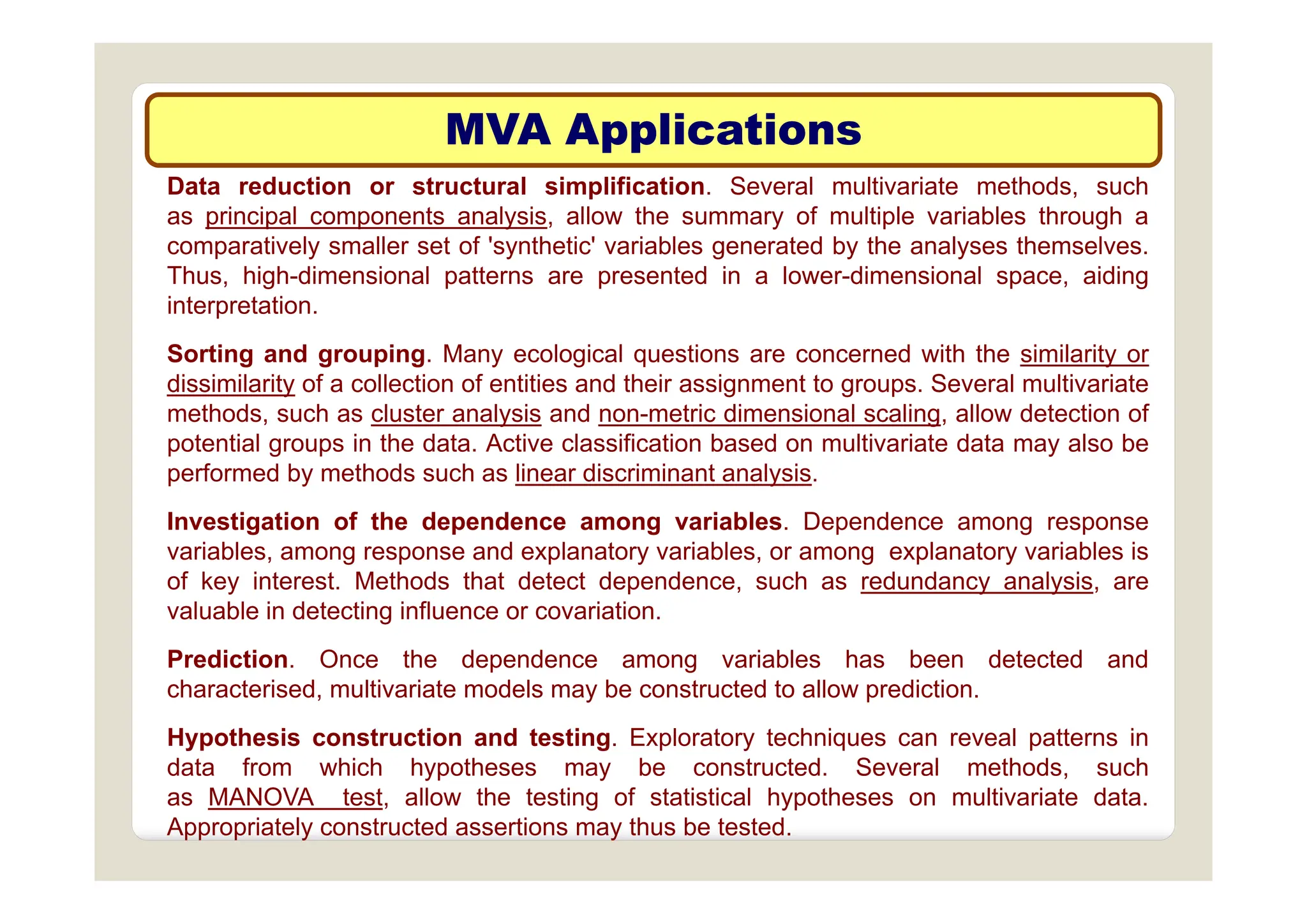
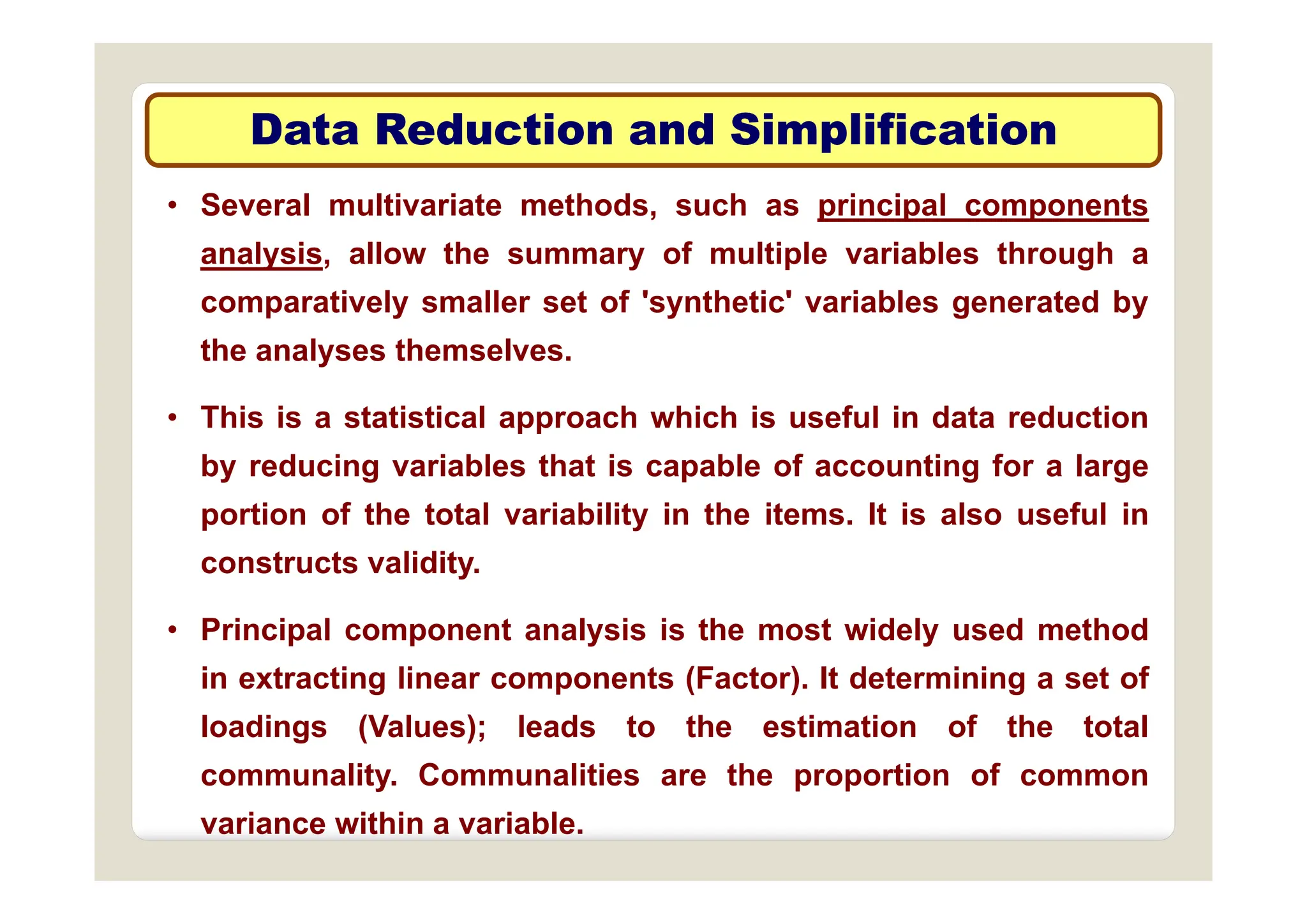
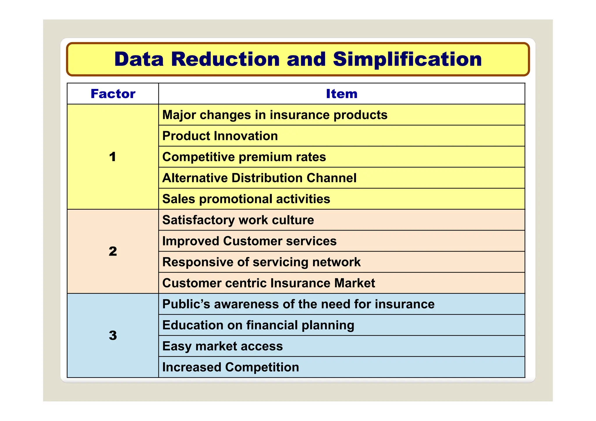
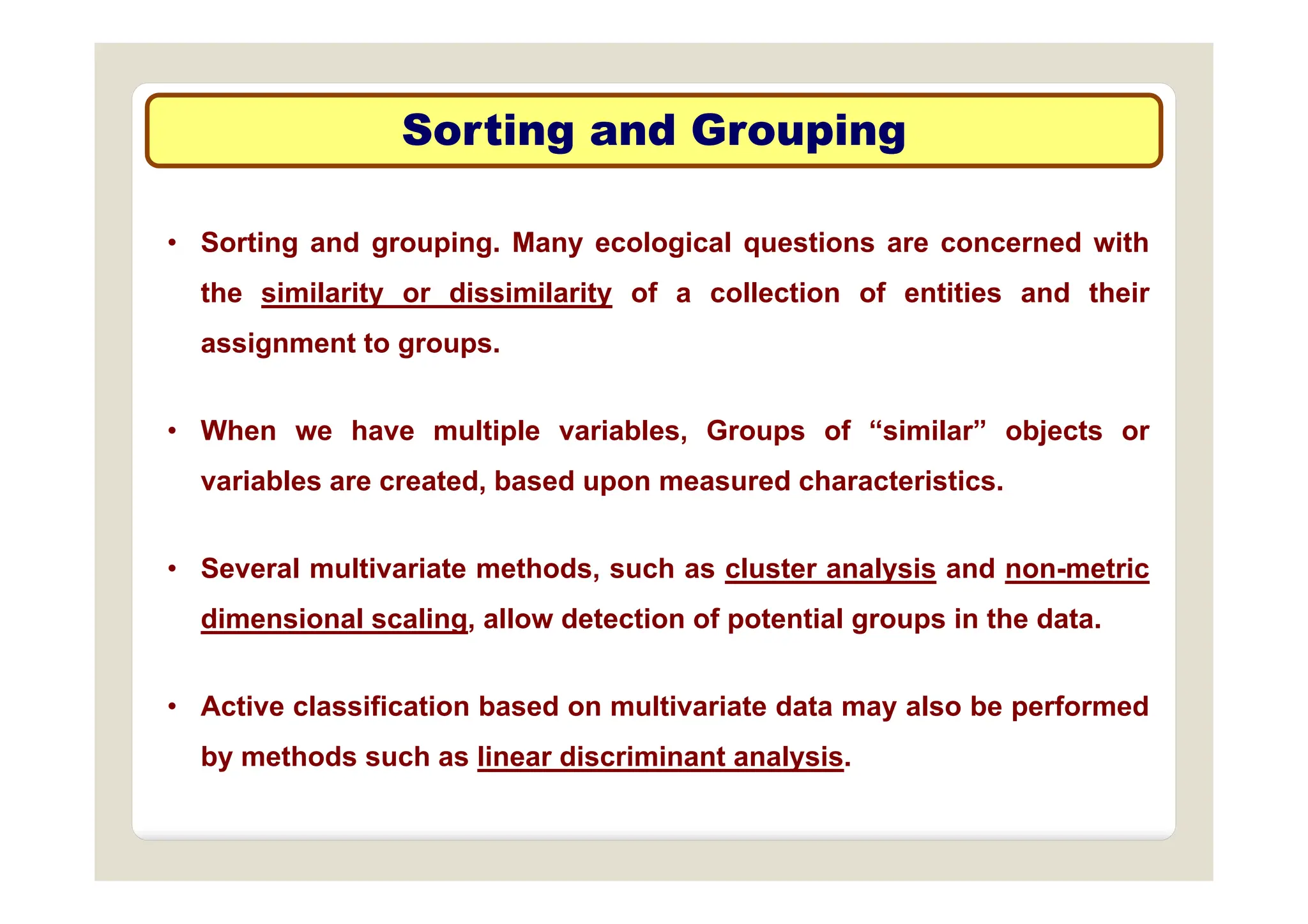
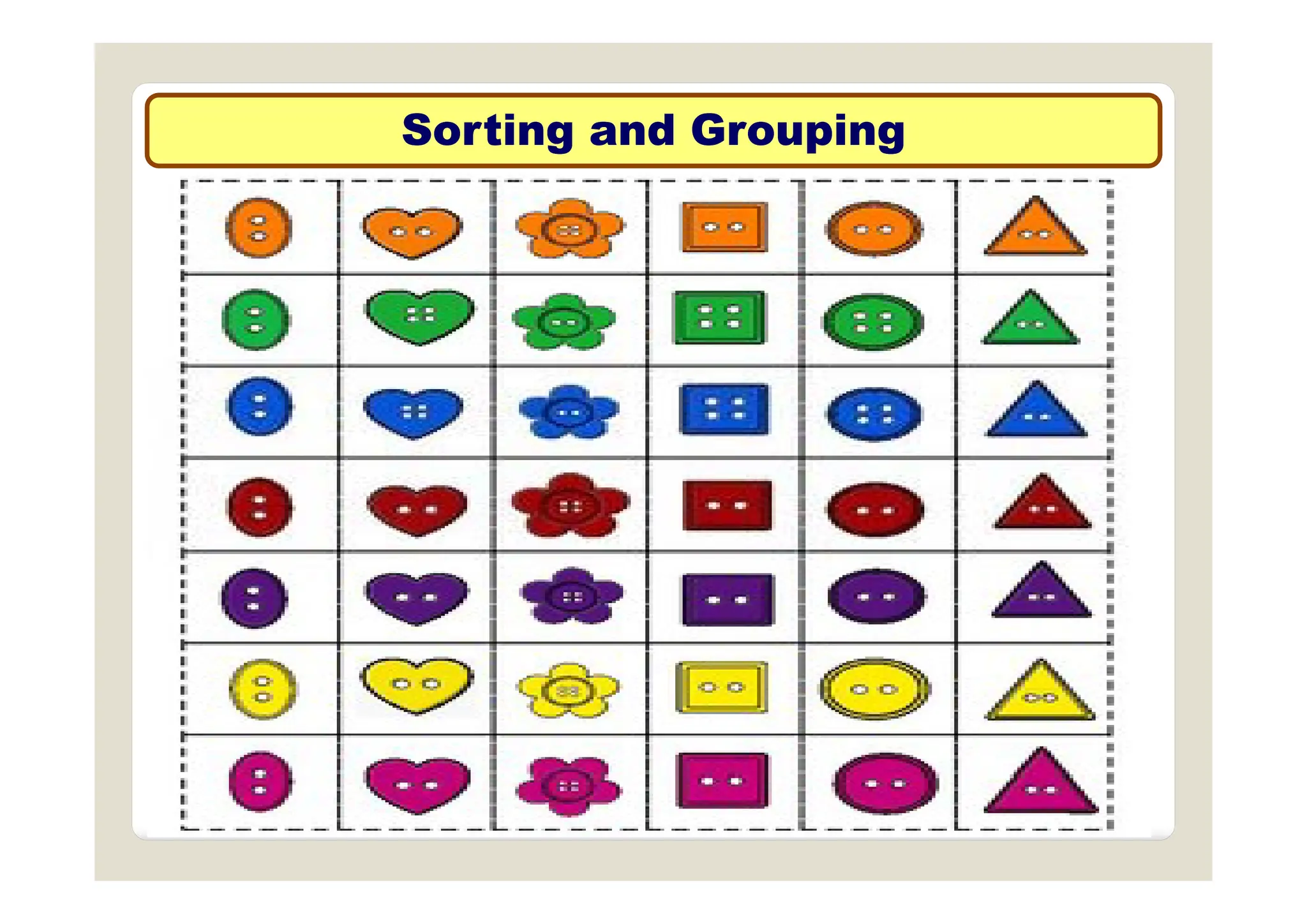
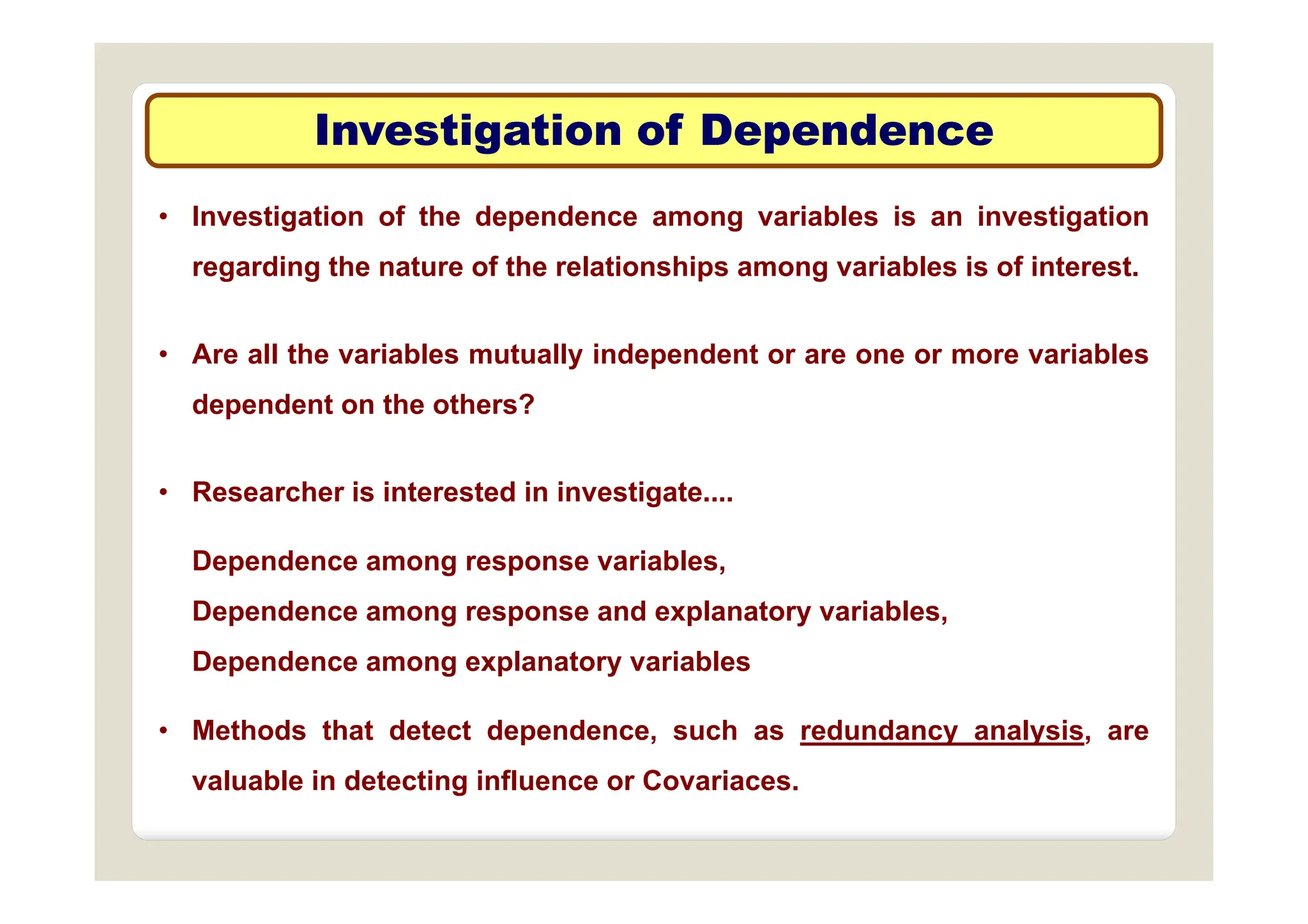
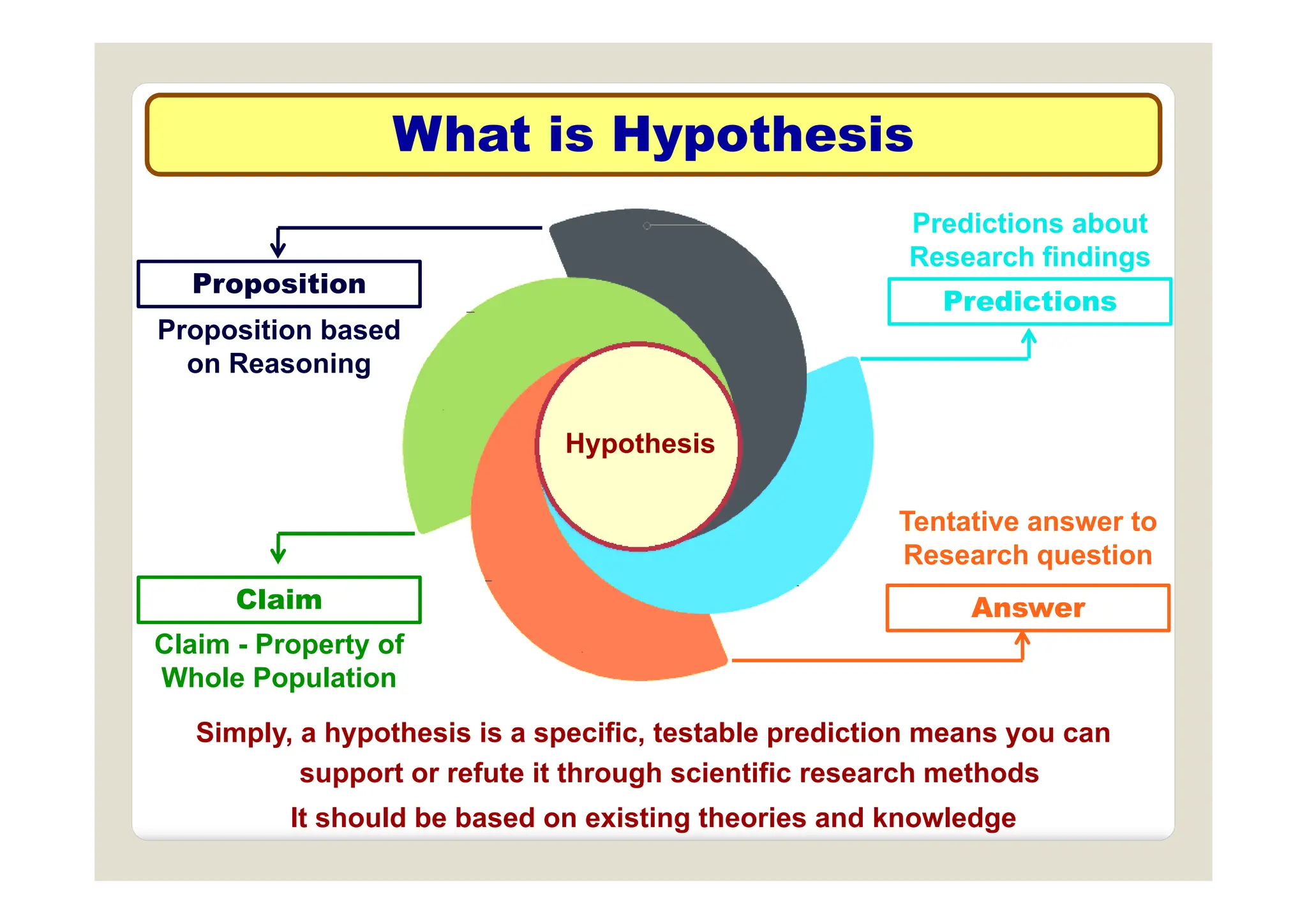
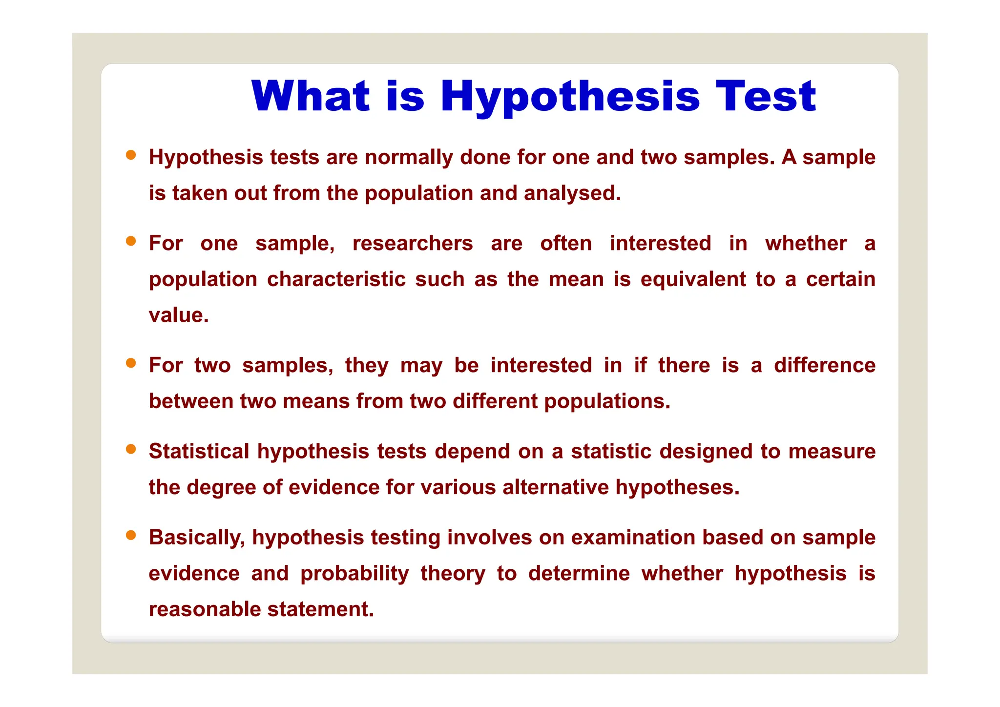
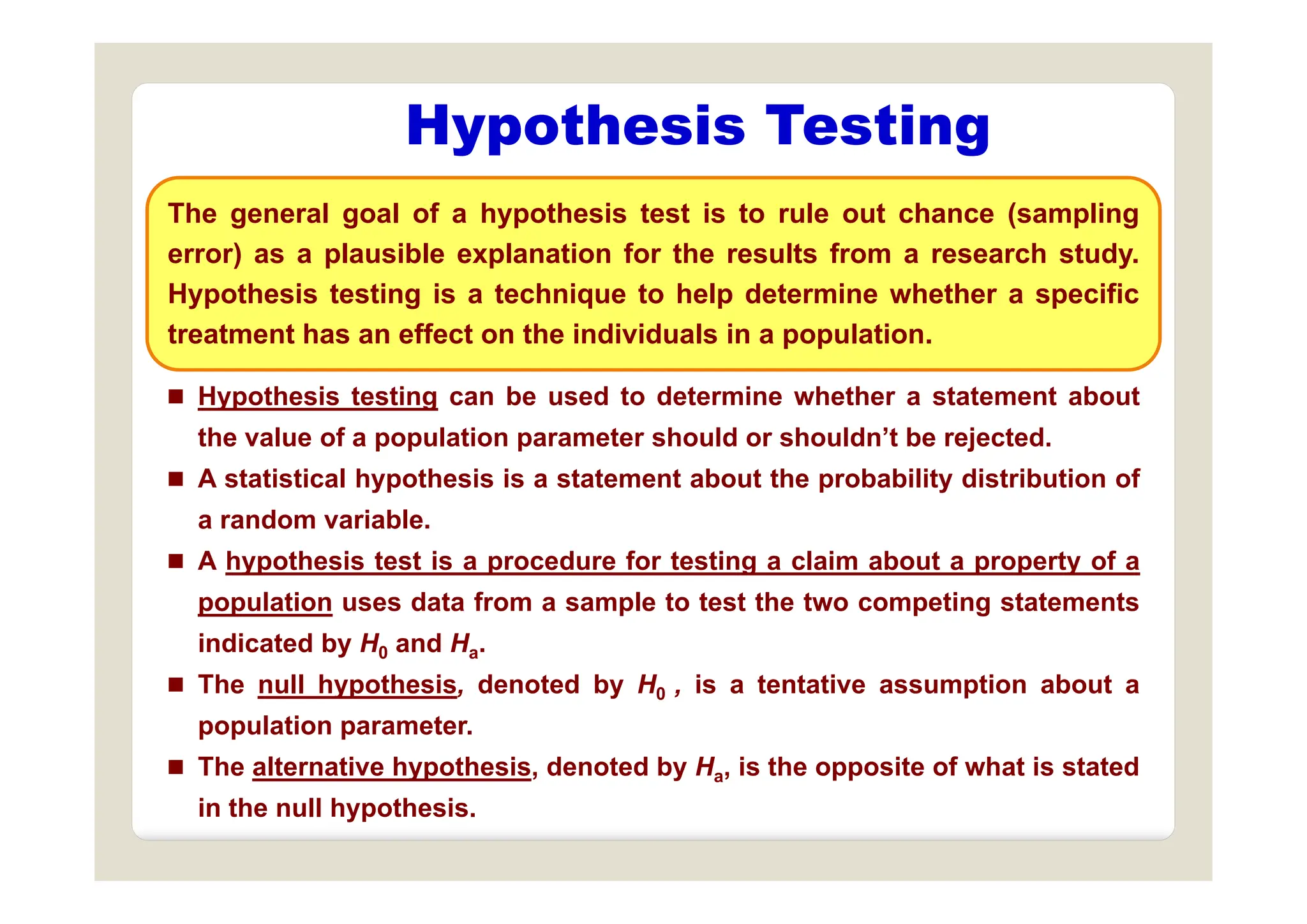
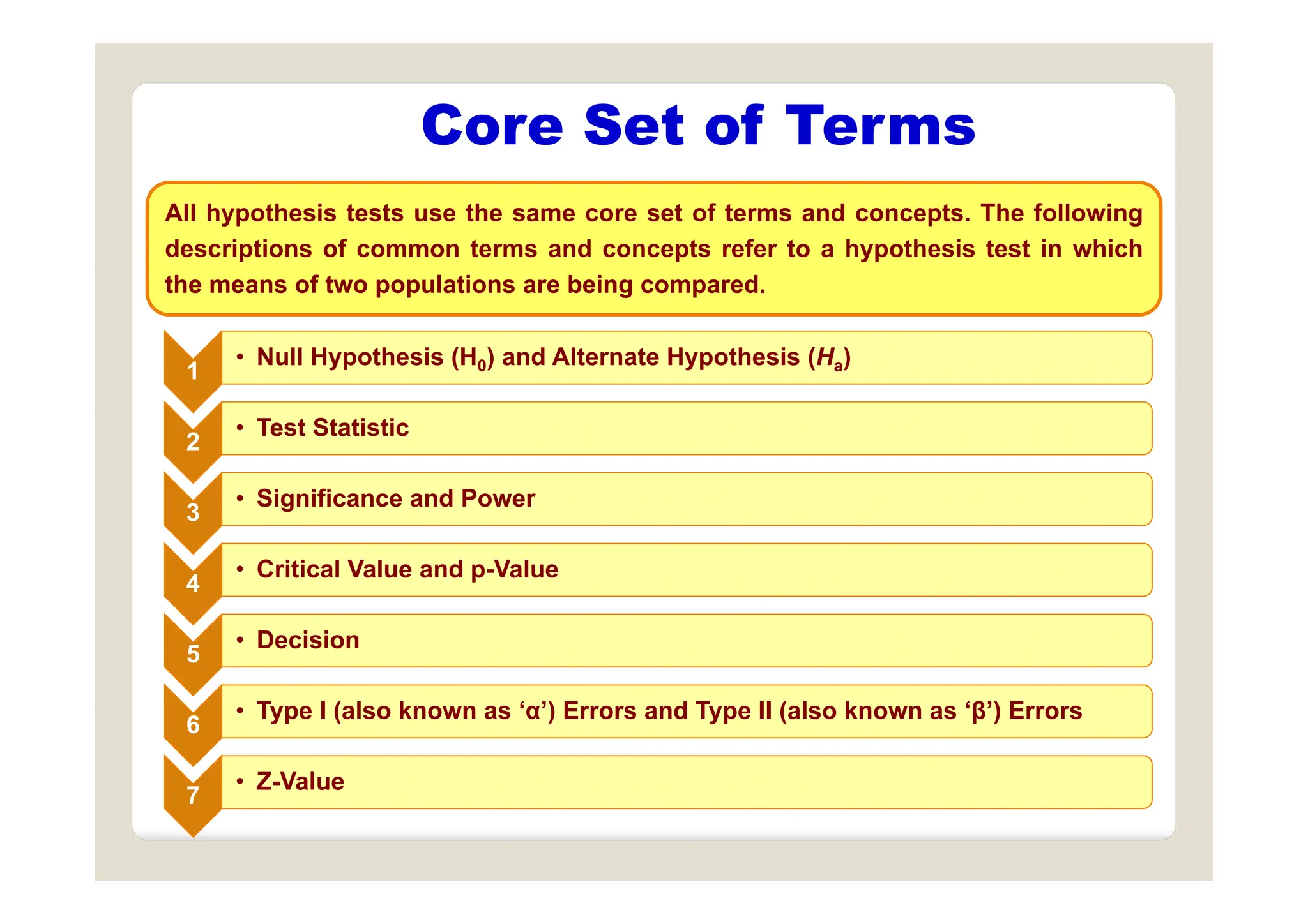
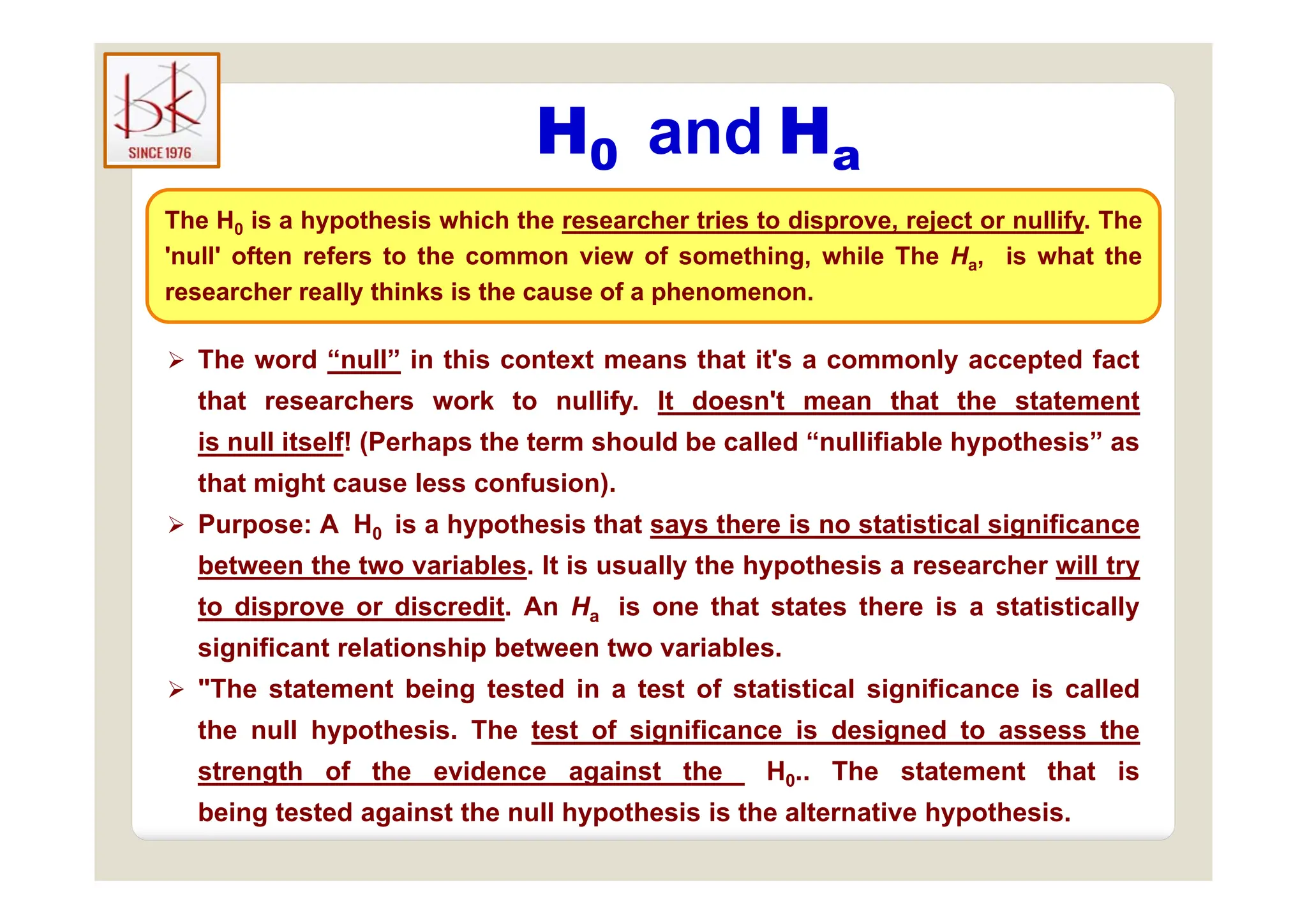
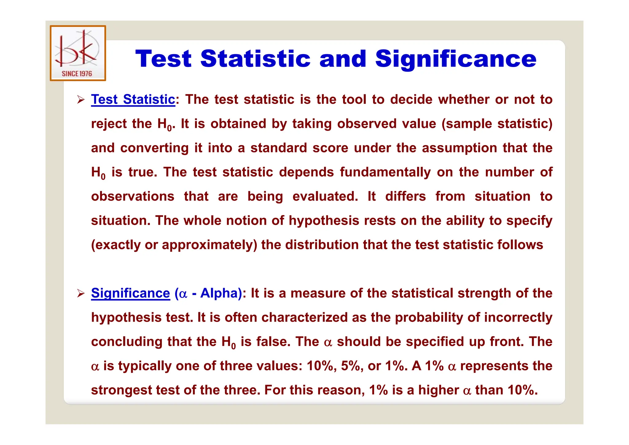
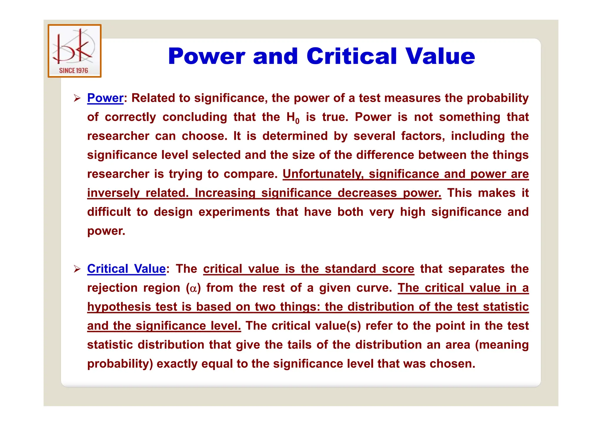
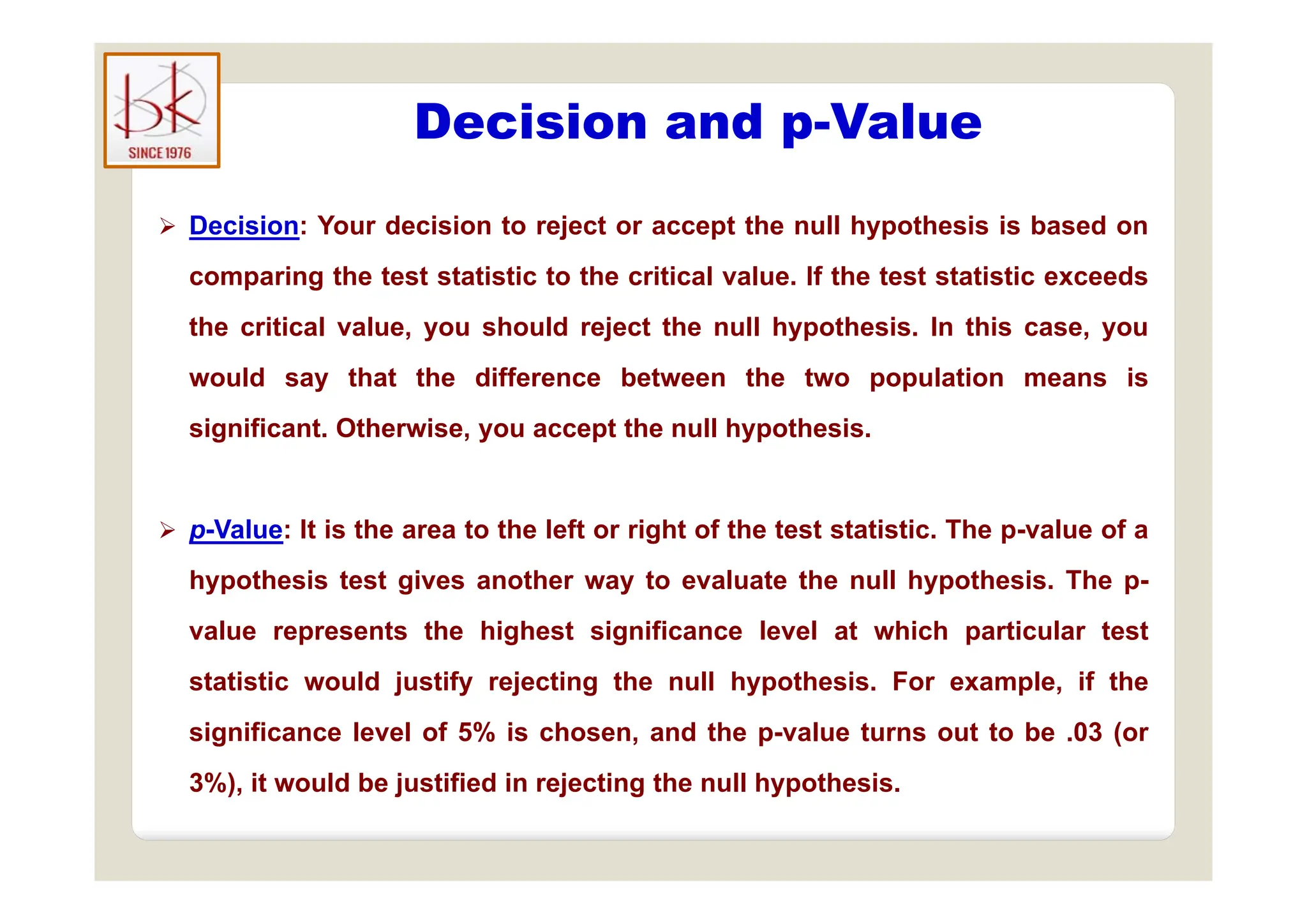
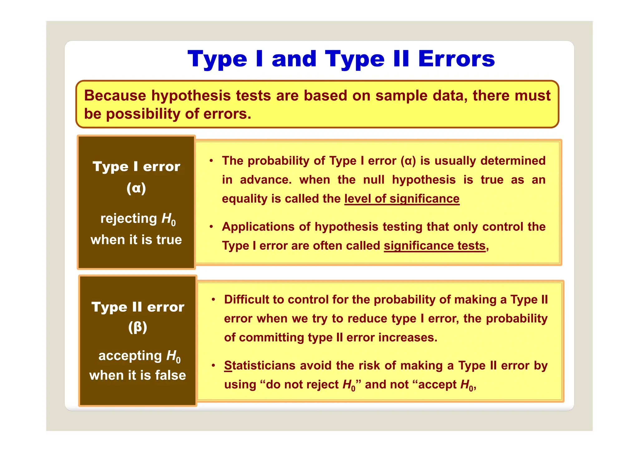
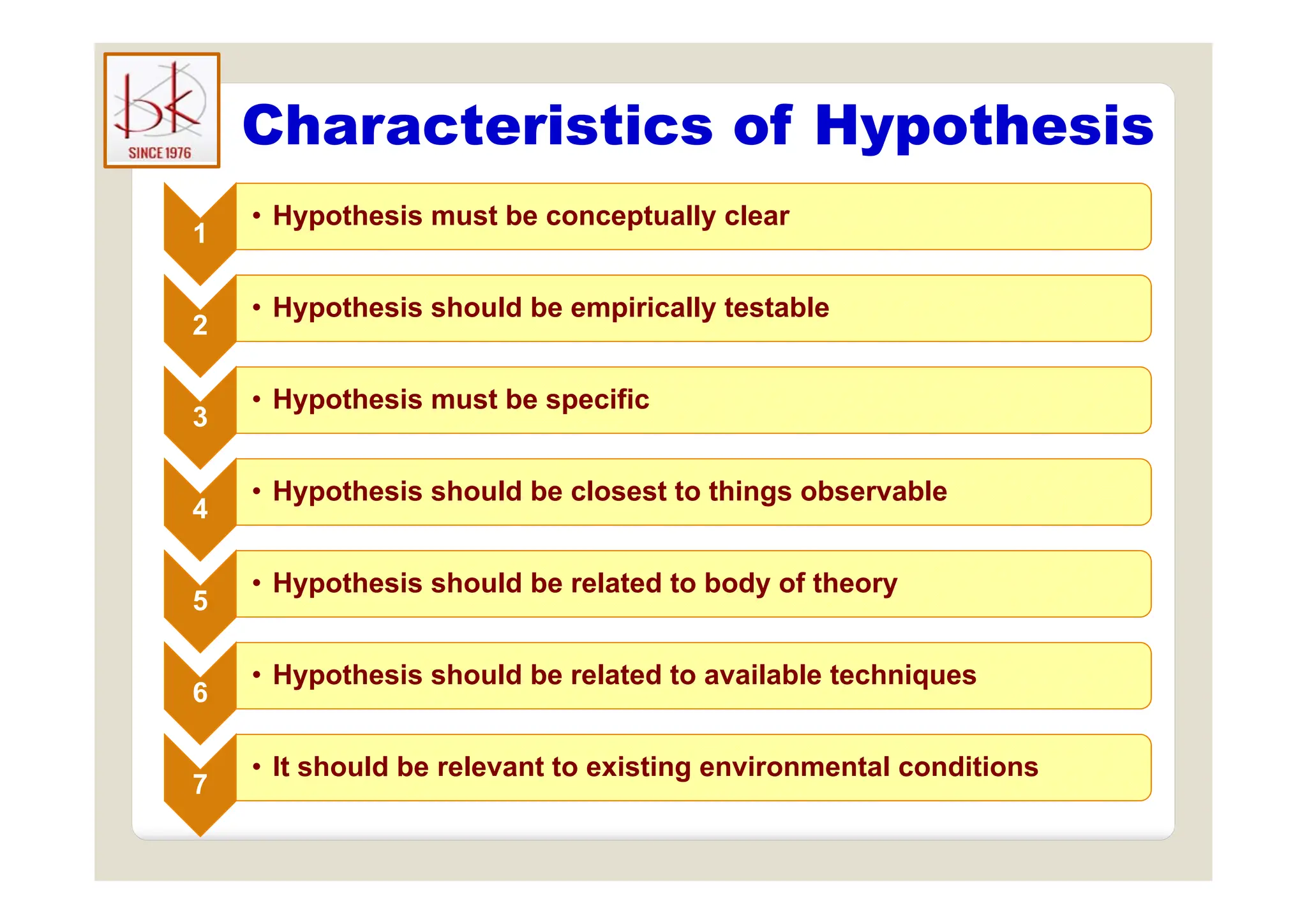
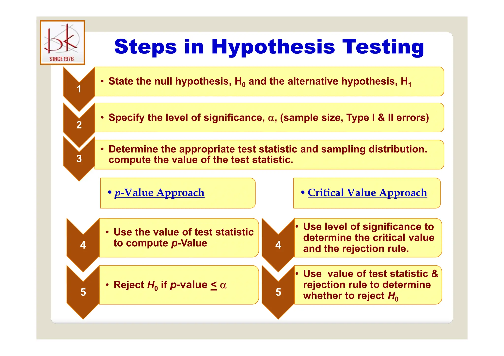
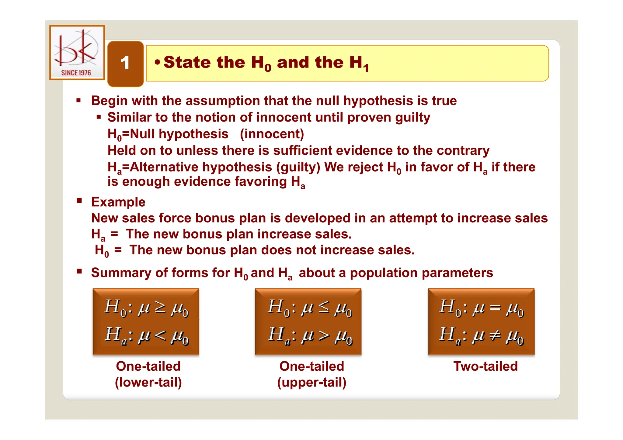
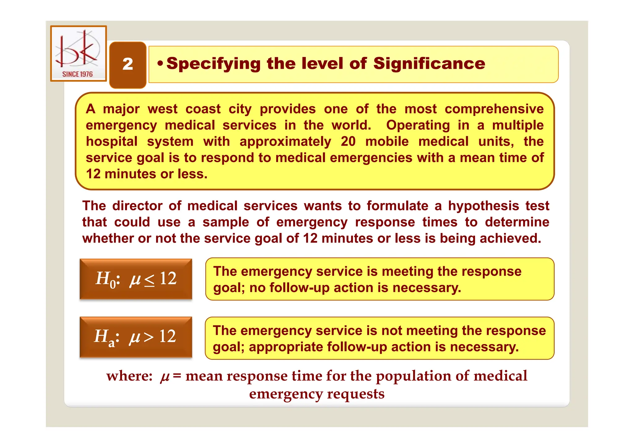
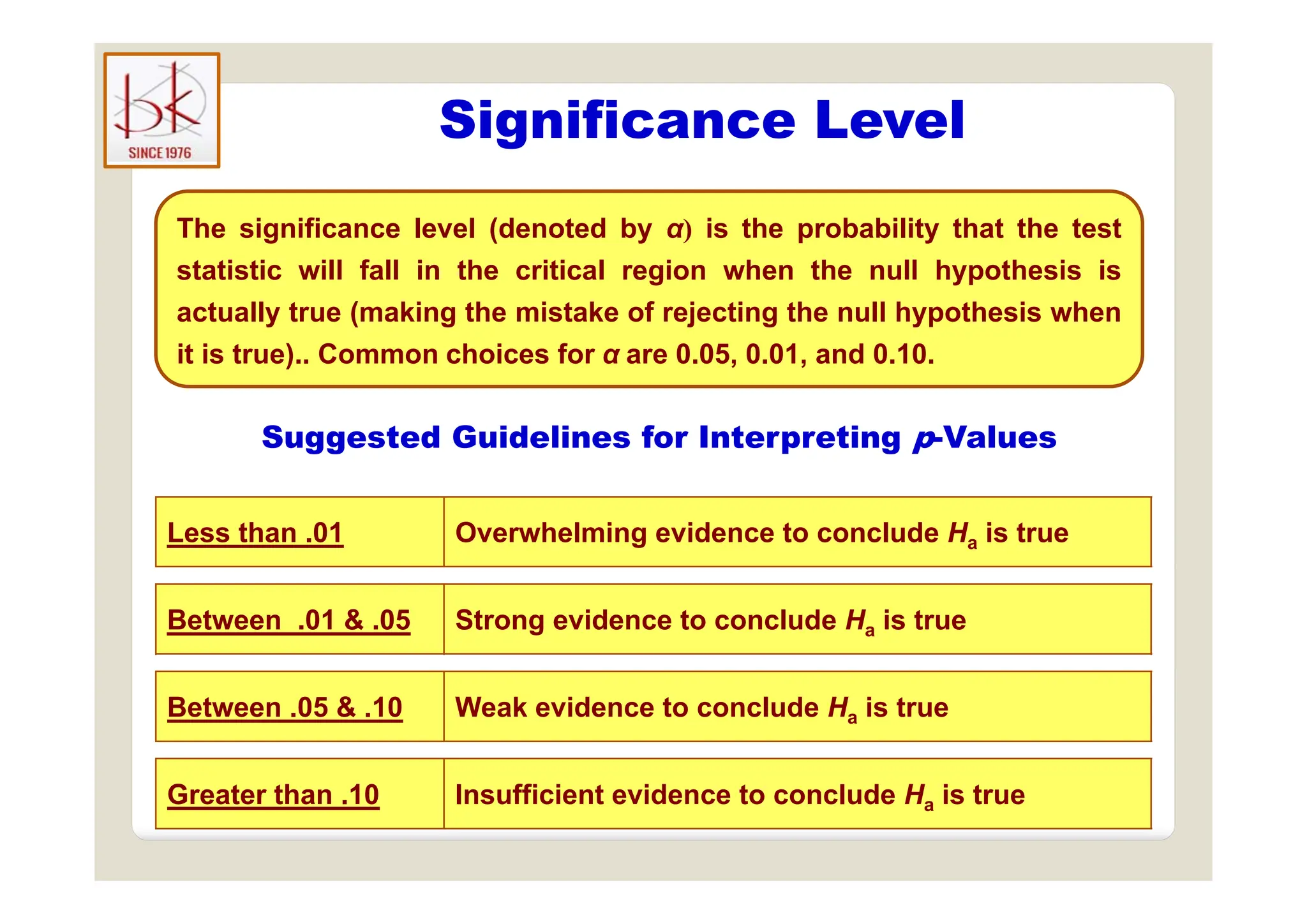
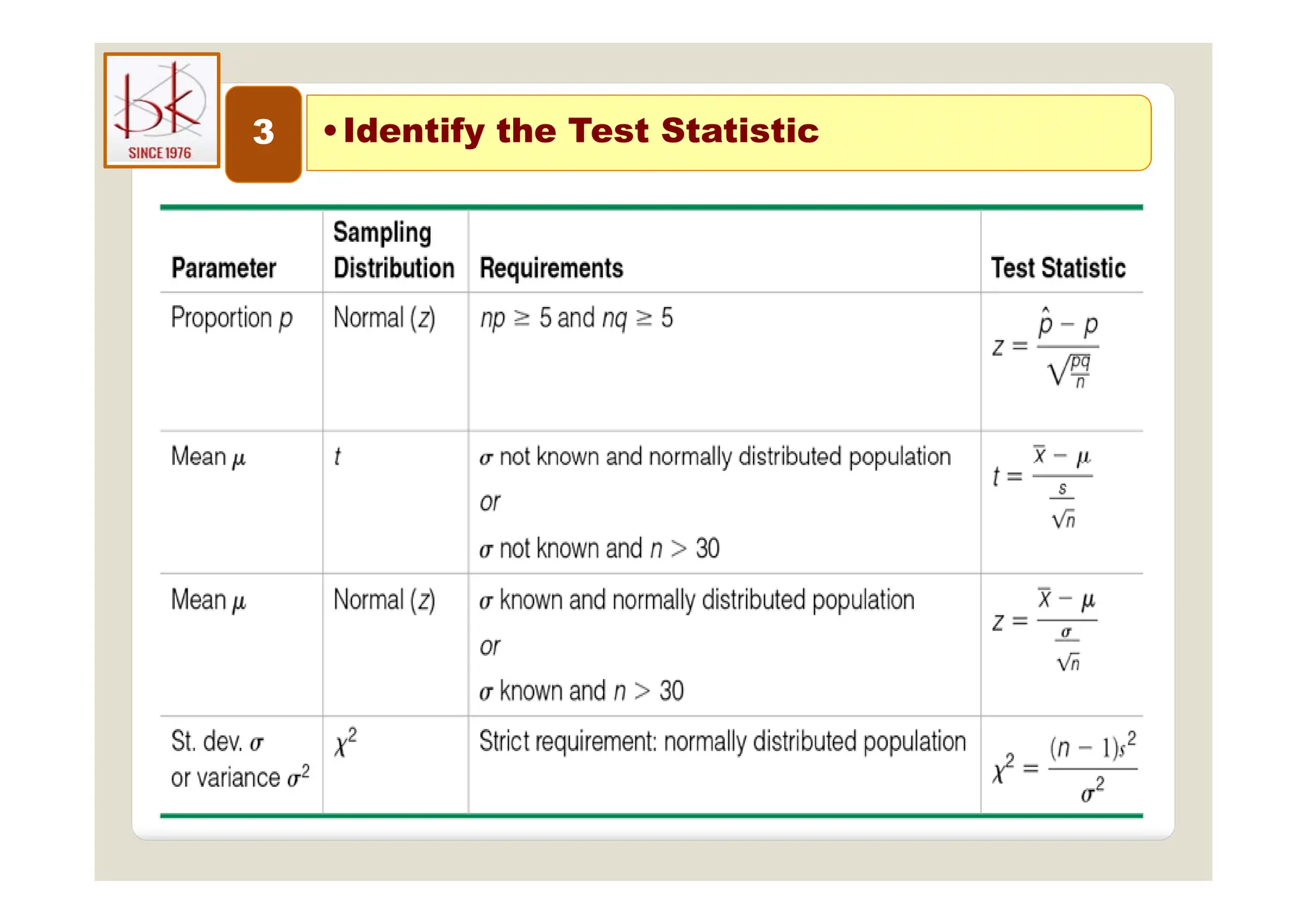
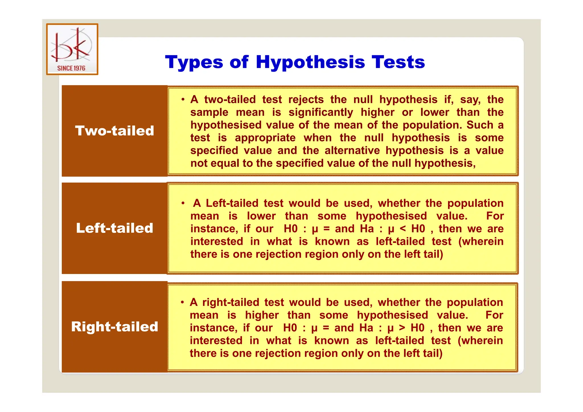
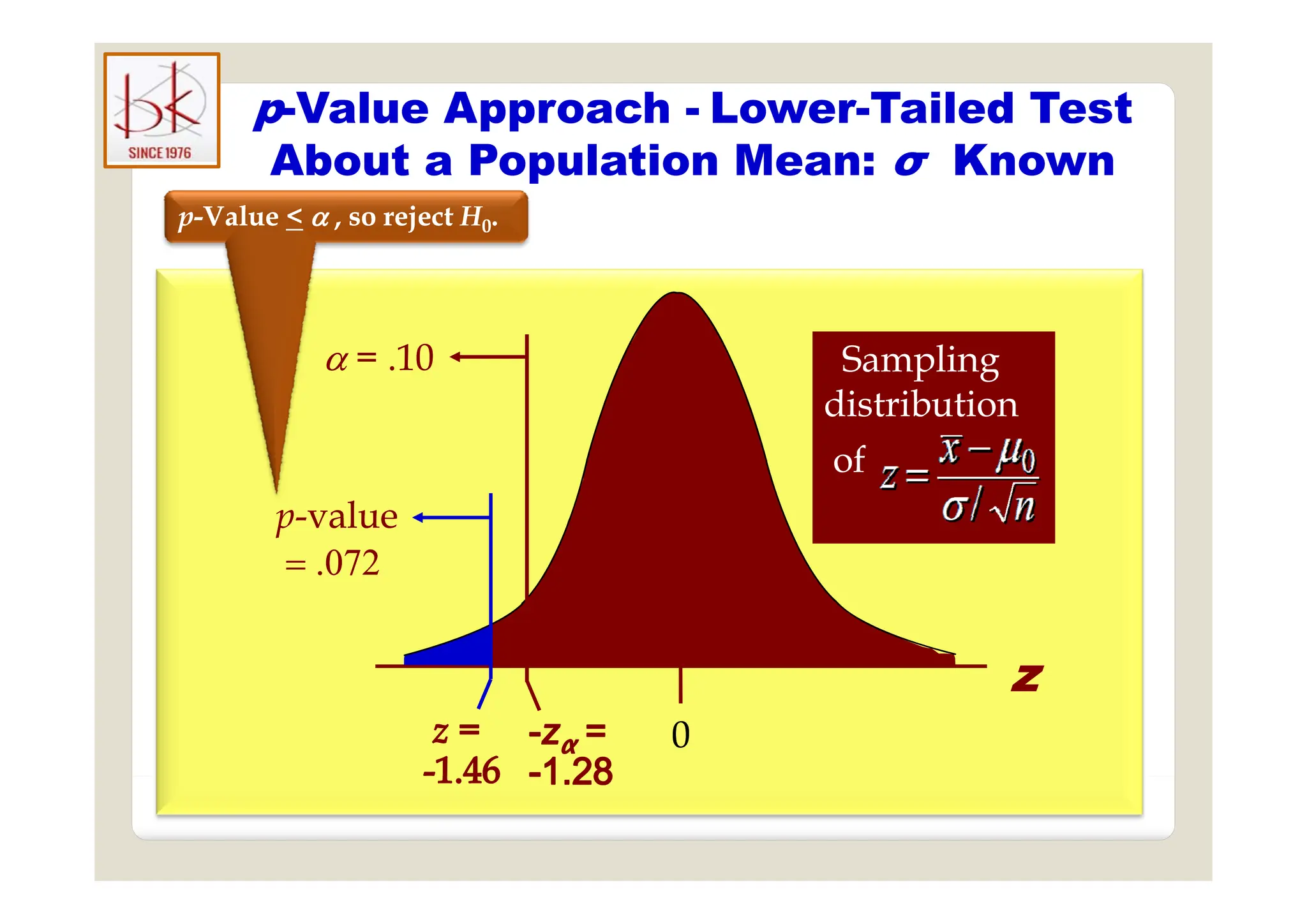
The document discusses multivariate data analysis and its applications in data reduction, sorting and grouping, dependence investigation, prediction, and hypothesis testing. Various statistical methods like principal components analysis, cluster analysis, and regression are examined for their role in summarizing data, detecting relationships, and making predictions. The document also covers important concepts related to hypothesis testing, including null and alternative hypotheses, test statistics, significance levels, and potential errors.

1. Multivariate Data Analysis
Multivariate Data Analysis
Dr. J D Chandrapal
MBA – marketing , PGDHRM, P HD, CII (Award) – London
g , , , ( )
Development Officer - LIC of India – Ahmedabad - 9825070933

2. MVA Applications
MVA Applications
pp
pp
Data reduction or structural simplification. Several multivariate methods, such
as principal components analysis, allow the summary of multiple variables through a
comparatively smaller set of 'synthetic' variables generated by the analyses themselves.
comparatively smaller set of synthetic variables generated by the analyses themselves.
Thus, high-dimensional patterns are presented in a lower-dimensional space, aiding
interpretation.
Sorting and grouping Many ecological questions are concerned with the similarity or
Sorting and grouping. Many ecological questions are concerned with the similarity or
dissimilarity of a collection of entities and their assignment to groups. Several multivariate
methods, such as cluster analysis and non-metric dimensional scaling, allow detection of
potential groups in the data. Active classification based on multivariate data may also be
performed by methods such as linear discriminant analysis.
Investigation of the dependence among variables. Dependence among response
variables, among response and explanatory variables, or among explanatory variables is
of key interest. Methods that detect dependence, such as redundancy analysis, are
valuable in detecting influence or covariation.
Prediction. Once the dependence among variables has been detected and
p g
characterised, multivariate models may be constructed to allow prediction.
Hypothesis construction and testing. Exploratory techniques can reveal patterns in
data from which hypotheses may be constructed. Several methods, such
yp y ,
as MANOVA test, allow the testing of statistical hypotheses on multivariate data.
Appropriately constructed assertions may thus be tested.

3. Data Reduction and Simplification
Data Reduction and Simplification
• Several multivariate methods, such as principal components
analysis allow the summary of multiple variables through a
p
p
analysis, allow the summary of multiple variables through a
comparatively smaller set of 'synthetic' variables generated by
the analyses themselves.
the analyses themselves.
• This is a statistical approach which is useful in data reduction
by reducing variables that is capable of accounting for a large
by reducing variables that is capable of accounting for a large
portion of the total variability in the items. It is also useful in
constructs validity
constructs validity.
• Principal component analysis is the most widely used method
i t ti li t (F t ) It d t i i t f
in extracting linear components (Factor). It determining a set of
loadings (Values); leads to the estimation of the total
communality Communalities are the proportion of common
communality. Communalities are the proportion of common
variance within a variable.

4. Data Reduction and Simplification
Data Reduction and Simplification
Factor Item
Major changes in insurance products
p
p
1
Major changes in insurance products
Product Innovation
Competitive premium rates
p p
Alternative Distribution Channel
Sales promotional activities
2
Satisfactory work culture
Improved Customer services
R i f i i t k
Responsive of servicing network
Customer centric Insurance Market
Public’s awareness of the need for insurance
3
Public s awareness of the need for insurance
Education on financial planning
Easy market access
Increased Competition

5. Sorting and Grouping
Sorting and Grouping
g p g
g p g
• Sorting and grouping. Many ecological questions are concerned with
g g p g y g q
the similarity or dissimilarity of a collection of entities and their
assignment to groups.
g g p
• When we have multiple variables, Groups of “similar” objects or
variables are created, based upon measured characteristics.
• Several multivariate methods such as cluster analysis and non metric
• Several multivariate methods, such as cluster analysis and non-metric
dimensional scaling, allow detection of potential groups in the data.
• Active classification based on multivariate data may also be performed
by methods such as linear discriminant analysis.

6. Sorting and Grouping
Sorting and Grouping
g p g
g p g

7. Investigation of Dependence
Investigation of Dependence
g p
g p
• Investigation of the dependence among variables is an investigation
regarding the nature of the relationships among variables is of interest.
• Are all the variables mutually independent or are one or more variables
• Are all the variables mutually independent or are one or more variables
dependent on the others?
• Researcher is interested in investigate....
Dependence among response variables,
Dependence among response variables,
Dependence among response and explanatory variables,
Dependence among explanatory variables
p g p y
• Methods that detect dependence, such as redundancy analysis, are
valuable in detecting influence or Covariaces
valuable in detecting influence or Covariaces.

8. 9.0
7 0
8.0
6.0
7.0
es
4 0
5.0
Price
--- HNI
3.0
4.0
Fuel
--- Middle Class
1 0
2.0
1.0
1.0 2.0 3.0 4.0 5.0 6.0 7.0 8.0 9.0 10.0
Sale of Petrol Vehicles

9. Prediction
Prediction
• Once the dependence among variables has been detected and
h t i d lti i t d l b t t d t ll
characterised, multivariate models may be constructed to allow
prediction.
• Prediction techniques rely on a predictive equation; multiple regression
is, indeed, a prime multivariate analysis prediction technique.
• With predictive analysis, you can unfold and develop initiatives that will
not only enhance your various operational processes but also help you
gain an all-important edge on the competition.
• If you understand why a trend, pattern, or event happened through
data you will be able to develop an informed projection of how things
data, you will be able to develop an informed projection of how things
may unfold in particular areas of the business.

10. General Equation for Prediction in CLRM
• In another word it can be said that the prediction is a kind of estimate
that contains true value +/- Error
• so the general equation in regression analysis is
Outcomei = (Model) + Error
Outcomei = (Model) + Error
Model = a+bx
Where a = constant =
b = Parameter =
xi = Predictor = Value of IV or Explanatory Variable
Standard Error =

11. Anatomy of CLRM
• In regression the model we fit is linear, which means that we
summarize a trend in data set with a strait line
summarize a trend in data set with a strait line.
500
450
--
-- Residual = 100 Actual Data
400
350
--
--
es
(Car)
300
250
200
--
--
--
lized
Sale
Line of “Best” Fit
Actual Y
275
Predicted 200
150
100
--
--
Y
=
Rea
Y = a + b X
Intercept Coefficient
Dependent Independent
Predicted
Y
175
50
0
--
--
5
I
10 15 20 25
I I I I
30
0
I I
35
I
Intercept Coefficient
( - ) Residual
X = Ad Budget ̷ Linear (Actual Sales)
■ Actual Sale

12. Hypothesis
Hypothesis
yp
yp
• Hypothesis construction and testing. Once the dependence among
i bl h b d t t d d h t i d lti i t d l
variables has been detected and characterised, multivariate models
may be constructed to allow prediction.
• Prediction techniques rely on a predictive equation; multiple regression
is, indeed, a prime multivariate analysis prediction technique.
• With predictive analysis, you can unfold and develop initiatives that will
not only enhance your various operational processes but also help you
gain an all-important edge on the competition.
• If you understand why a trend, pattern, or event happened through
data you will be able to develop an informed projection of how things
data, you will be able to develop an informed projection of how things
may unfold in particular areas of the business.

13. What is Hypothesis
What is Hypothesis
Predictions about
Research findings
Research findings
Predictions
Proposition based
R i
Proposition
on Reasoning
Hypothesis
Tentative answer to
Research question
q
Answer
Claim - Property of
Wh l P l ti
Claim
Whole Population
Simply, a hypothesis is a specific, testable prediction means you can
support or refute it through scientific research methods
support or refute it through scientific research methods
It should be based on existing theories and knowledge

14. What is Hypothesis Test
 Hypothesis tests are normally done for one and two samples. A sample
is taken out from the population and analysed
yp
is taken out from the population and analysed.
 For one sample, researchers are often interested in whether a
l ti h t i ti h th i i l t t t i
population characteristic such as the mean is equivalent to a certain
value.
 For two samples, they may be interested in if there is a difference
between two means from two different populations.
 Statistical hypothesis tests depend on a statistic designed to measure
the degree of evidence for various alternative hypotheses.
 Basically, hypothesis testing involves on examination based on sample
evidence and probability theory to determine whether hypothesis is
reasonable statement.

15. Hypothesis Testing
yp g
The general goal of a hypothesis test is to rule out chance (sampling
error) as a plausible explanation for the results from a research study
error) as a plausible explanation for the results from a research study.
Hypothesis testing is a technique to help determine whether a specific
treatment has an effect on the individuals in a population.
 Hypothesis testing can be used to determine whether a statement about
the value of a population parameter should or shouldn’t be rejected.
 A statistical hypothesis is a statement about the probability distribution of
a random variable.
 A hypothesis test is a procedure for testing a claim about a property of a
 A hypothesis test is a procedure for testing a claim about a property of a
population uses data from a sample to test the two competing statements
indicated by H0 and Ha.
 The null hypothesis, denoted by H0 , is a tentative assumption about a
population parameter.
 The alternative hypothesis, denoted by Ha, is the opposite of what is stated
yp , y a, pp
in the null hypothesis.

16. Core Set of Terms
All hypothesis tests use the same core set of terms and concepts. The following
descriptions of common terms and concepts refer to a hypothesis test in which
descriptions of common terms and concepts refer to a hypothesis test in which
the means of two populations are being compared.
• Null Hypothesis (H ) and Alternate Hypothesis (H )
1
1
• Null Hypothesis (H0) and Alternate Hypothesis (Ha)
2
2
• Test Statistic
3
3
• Significance and Power
• Critical Value and p Value
4
4
• Critical Value and p-Value
5
5
• Decision
6
6
• Type I (also known as ‘α’) Errors and Type II (also known as ‘β’) Errors
Z V l
7
7
• Z-Value

17. H0 and Ha
H0 and Ha
The H0 is a hypothesis which the researcher tries to disprove, reject or nullify. The
'null' often refers to the common view of something while The H is what the
 The word “null” in this context means that it's a commonly accepted fact
'null' often refers to the common view of something, while The Ha, is what the
researcher really thinks is the cause of a phenomenon.
 The word “null” in this context means that it s a commonly accepted fact
that researchers work to nullify. It doesn't mean that the statement
is null itself! (Perhaps the term should be called “nullifiable hypothesis” as
that might cause less confusion).
 Purpose: A H0 is a hypothesis that says there is no statistical significance
between the two variables It is usually the hypothesis a researcher will try
between the two variables. It is usually the hypothesis a researcher will try
to disprove or discredit. An Ha is one that states there is a statistically
significant relationship between two variables.
 "The statement being tested in a test of statistical significance is called
the null hypothesis. The test of significance is designed to assess the
strength of the evidence against the H0 The statement that is
strength of the evidence against the H0.. The statement that is
being tested against the null hypothesis is the alternative hypothesis.

18. Test Statistic and Significance
g
 Test Statistic: The test statistic is the tool to decide whether or not to
reject the H It is obtained by taking observed value (sample statistic)
reject the H0. It is obtained by taking observed value (sample statistic)
and converting it into a standard score under the assumption that the
H is true The test statistic depends fundamentally on the number of
H0 is true. The test statistic depends fundamentally on the number of
observations that are being evaluated. It differs from situation to
situation The whole notion of hypothesis rests on the ability to specify
situation. The whole notion of hypothesis rests on the ability to specify
(exactly or approximately) the distribution that the test statistic follows
 Significance ( - Alpha): It is a measure of the statistical strength of the
hypothesis test. It is often characterized as the probability of incorrectly
yp p y y
concluding that the H0 is false. The  should be specified up front. The
 is typically one of three values: 10%, 5%, or 1%. A 1%  represents the
strongest test of the three. For this reason, 1% is a higher  than 10%.

19. Power and Critical Value
 Power: Related to significance, the power of a test measures the probability
of correctly concluding that the H is true Power is not something that
of correctly concluding that the H0 is true. Power is not something that
researcher can choose. It is determined by several factors, including the
significance level selected and the size of the difference between the things
researcher is trying to compare. Unfortunately, significance and power are
inversely related. Increasing significance decreases power. This makes it
difficult to design experiments that have both very high significance and
difficult to design experiments that have both very high significance and
power.
 Critical Value: The critical value is the standard score that separates the
rejection region () from the rest of a given curve. The critical value in a
hypothesis test is based on two things: the distribution of the test statistic
hypothesis test is based on two things: the distribution of the test statistic
and the significance level. The critical value(s) refer to the point in the test
statistic distribution that give the tails of the distribution an area (meaning
probability) exactly equal to the significance level that was chosen.

20. Decision and p-Value
p
 Decision: Your decision to reject or accept the null hypothesis is based on
comparing the test statistic to the critical value. If the test statistic exceeds
the critical value, you should reject the null hypothesis. In this case, you
would say that the difference between the two population means is
significant. Otherwise, you accept the null hypothesis.
 p-Value: It is the area to the left or right of the test statistic. The p-value of a
hypothesis test gives another way to evaluate the null hypothesis. The p-
value represents the highest significance level at which particular test
f f
statistic would justify rejecting the null hypothesis. For example, if the
significance level of 5% is chosen, and the p-value turns out to be .03 (or
3%) it ld b j tifi d i j ti th ll h th i
3%), it would be justified in rejecting the null hypothesis.

21. Type I and Type II Errors
Because hypothesis tests are based on sample data, there must
be possibility of errors.
• The probability of Type I error (α) is usually determined
Type I error
in advance. when the null hypothesis is true as an
equality is called the level of significance
• Applications of hypothesis testing that only control the
(α)
rejecting H0 • Applications of hypothesis testing that only control the
Type I error are often called significance tests,
0
when it is true
• Difficult to control for the probability of making a Type II
error when we try to reduce type I error, the probability
Type II error
(β)
of committing type II error increases.
• Statisticians avoid the risk of making a Type II error by
“ “
(β)
accepting H0
when it is false
using “do not reject H0” and not “accept H0,
when it is false

22. Type I and Type II Errors
Population Condition
H0 True
(The drug doesn’t work)
H0 False
(The drug works)
Conclusion
Correct
Decision Type II Error
Accept H0 Decision
1 - α
Type II Error
Correct
Accept H0
Correct
Decision
1 - β
Type I Error
Reject H0
False Negative False Positive
Goal: Keep , reasonably small
22
Error)
II
P(Type
β
Error)
I
P(Type
α 


23. Z-Value
 Z value is a measure of standard deviation (σ) i.e. how many SD(σ) away
from mean is the observed value.
 z-score is a very useful statistic because it allows us to calculate the
probability of a score occurring within our normal distribution.
 Z-scores range from -3 SD(σ) (which would fall to the far left of the normal
distribution curve) up to +3 SD(σ) (which would fall to the far right of the
normal distribution curve)
normal distribution curve).
 In order to use a z-score, you need to know the mean μ and also the
population std deviation σ.
 Technically, z-scores are a conversion of individual scores into a standard
form. The conversion allows you to more easily compare different data; it is
b d k l d b t th l ti ’ t d d d i ti d
based on your knowledge about the population’s standard deviation and
mean. A z-score tells you how many SD(σ) from the mean your result is..
 The z-score formula doesn’t say anything about sample size; The rule of
 The z score formula doesn t say anything about sample size; The rule of
thumb applies that your sample size should be above 30 to use it.

24. Z-Value and t-Value
 The t Statistic is used in a t test when you are deciding if you should support or
reject the null hypothesis It’s very similar to a Z-score
reject the null hypothesis. It s very similar to a Z-score
 The Z score is scaled down by the population std deviation (σ). The t score is
scaled down by the sample std deviation (s). You usually have the latter, not so
much the former However due to the central limit theorem in most cases with a
much the former. However, due to the central limit theorem in most cases with a
very large sample of means you can assume normality and use the Z score.
 In order to use Z, we must know four things:
• The population mean
• The population mean.
• The population standard deviation.
• The sample mean.
The sample size
• The sample size.
Usually in stats, you don’t know anything about a population, so instead of a Z
score you use a t Test with a t Statistic. The major difference between using a Z
d t t ti ti i th t h t ti t th l ti t d d
score and a t statistic is that you have to estimate the population standard
deviation. The t test is also used if you have a small sample size (less than 30).
 The greater the t, the more evidence you have that your observations are
i ifi l diff f A ll l i id h
significantly different from average. A smaller t value is evidence that your
observations are not significantly different from average. :

25. When to use a t score
I l i Yes
Use the Z-Score
Do you know the
population Std
D i i
Yes
N
Is sample size
above 30?
Yes
No Use the t-Score
Deviation σ No
Use the t Score
Z-Value for Proportion Z-Value for Mean t-Value for Mean
σ known and normally σ unknown & normally
np ≥ 5 and
nq ≥ 5
σ known and normally
distributed population
or
σ unknown & normally
distributed population
or
nq ≥ 5
σ known and n>30 σ known and n<30

26. Characteristics of Hypothesis
yp
1
1
• Hypothesis must be conceptually clear
2
2
• Hypothesis should be empirically testable
3
3
• Hypothesis must be specific
4
4
• Hypothesis should be closest to things observable
5
5
• Hypothesis should be related to body of theory
• Hypothesis should be related to available techniques
6
6
• Hypothesis should be related to available techniques
7
7
• It should be relevant to existing environmental conditions
7
t s ou d be e e a t to e st g e o e ta co d t o s

27. Steps in Hypothesis Testing
1
• State the null hypothesis, H0 and the alternative hypothesis, H1
p yp g
2
• Specify the level of significance, , (sample size, Type I & II errors)
3
• Determine the appropriate test statistic and sampling distribution.
compute the value of the test statistic.
•p-Value Approach •Critical Value Approach
4
• Use the value of test statistic
to compute p-Value 4
• Use level of significance to
determine the critical value
and the rejection rule.
5
• Reject H0 if p-value < 
5
• Use value of test statistic &
rejection rule to determine
whether to reject H0
et e to eject 0

28. 1 •State the H0 and the H1
0 1
 Begin with the assumption that the null hypothesis is true
 Similar to the notion of innocent until proven guilty
Similar to the notion of innocent until proven guilty
H0=Null hypothesis (innocent)
Held on to unless there is sufficient evidence to the contrary
Ha=Alternative hypothesis (guilty) We reject H0 in favor of Ha if there
Ha Alternative hypothesis (guilty) We reject H0 in favor of Ha if there
is enough evidence favoring Ha
 Example
New sales force bonus plan is developed in an attempt to increase sales
New sales force bonus plan is developed in an attempt to increase sales
Ha = The new bonus plan increase sales.
H0 = The new bonus plan does not increase sales.
 S f f f H d H b t l ti t
 Summary of forms for H0 and Ha about a population parameters
One-tailed One-tailed Two-tailed
One tailed
(lower-tail)
One tailed
(upper-tail)
Two tailed

29. 2 •Specifying the level of Significance
p y g g
A major west coast city provides one of the most comprehensive
di l i i th ld O ti i lti l
emergency medical services in the world. Operating in a multiple
hospital system with approximately 20 mobile medical units, the
service goal is to respond to medical emergencies with a mean time of
12 minutes or less
12 minutes or less.
The director of medical services wants to formulate a hypothesis test
that could use a sample of emergency response times to determine
that could use a sample of emergency response times to determine
whether or not the service goal of 12 minutes or less is being achieved.
The emergency service is meeting the response
H
H 


 The emergency service is meeting the response
goal; no follow-up action is necessary.
Th i i t ti th
H
H0
0:
: 




The emergency service is not meeting the response
goal; appropriate follow-up action is necessary.
Ha:
where:  = mean response time for the population of medical
where:  = mean response time for the population of medical
emergency requests

30. Significance Level
g
The significance level (denoted by α) is the probability that the test
statistic will fall in the critical region when the null hypothesis is
actually true (making the mistake of rejecting the null hypothesis when
it is true) Common choices for α are 0 05 0 01 and 0 10
Suggested Guidelines for Interpreting p-Values
it is true).. Common choices for α are 0.05, 0.01, and 0.10.
Less than .01 Overwhelming evidence to conclude Ha is true
Between .01 & .05 Strong evidence to conclude Ha is true
Between .05 & .10 Weak evidence to conclude Ha is true
Greater than .10 Insufficient evidence to conclude Ha is true

31. 3 •Identify the Test Statistic
y

32. Types of Hypothesis Tests
Types of Hypothesis Tests
• A two-tailed test rejects the null hypothesis if, say, the
sample mean is significantly higher or lower than the
sample mean is significantly higher or lower than the
hypothesised value of the mean of the population. Such a
test is appropriate when the null hypothesis is some
specified value and the alternative hypothesis is a value
t l t th ifi d l f th ll h th i
Two-tailed
not equal to the specified value of the null hypothesis,
• A Left-tailed test would be used, whether the population
A Left tailed test would be used, whether the population
mean is lower than some hypothesised value. For
instance, if our H0 : µ = and Ha : µ < H0 , then we are
interested in what is known as left-tailed test (wherein
there is one rejection region only on the left tail)
Left-tailed
there is one rejection region only on the left tail)
A i ht t il d t t ld b d h th th l ti
• A right-tailed test would be used, whether the population
mean is higher than some hypothesised value. For
instance, if our H0 : µ = and Ha : µ > H0 , then we are
interested in what is known as left-tailed test (wherein
Right-tailed
(
there is one rejection region only on the left tail)

33. p-Value Approach - Lower-Tailed Test
Ab t P l ti M K
About a Population Mean: σ Known
p
p-
-Value
Value <
< 
 , so
, so reject
reject H
H0
0.
.
 = 10
 = 10 Sampling
Sampling
 = .10
 = .10 Sampling
distribution
of
Sampling
distribution
of
p-value
 
p-value
 
of
of


z
z
0
0
z
z

34. p-Value Approach - Upper-Tailed Test
Ab t P l ti M K
About a Population Mean:σ Known
p
p-
-Value
Value <
< 
 , so
, so reject
reject H
H0
0.
.
Sampling
Sampling
 = .04
 = .04
distribution
of
distribution
of
p-Value
p-Value


0
0
z
z

35. Critical Value Approach
One-Tailed Hypothesis Testing
 The test statistic z has a standard normal probability
 The test statistic z has a standard normal probability
distribution.
 We can use the standard normal probability distribution table to
 We can use the standard normal probability distribution table to
find the z-value with an area of a in the lower (or upper) tail of
the distribution.
the distribution.
 The value of the test statistic that established the boundary of
the rejection region is called the critical value for the test
the rejection region is called the critical value for the test.

 The rejection rule is:
The rejection rule is:
j
j
•
• Lower tail: Reject H0 if z < -z
• Upper tail: Reject H0 if z > z
pp j 0 

36. Critical Value Approach - Lower-Tailed Test
Ab t P l ti M K
About a Population Mean :  Known
Sampling
Di t ib ti
Sampling
Di t ib ti
Distribution
of
Distribution
of
of
of

37. Critical Value Approach
Upper-Tailed Test :  Known
Sampling
Sampling
distribution
of
distribution
of

38. Here are some common values
Confidence Area between Area in one z-score
Here are some common values
Confidence
Level
Area between
0 and z-score
Area in one
tail (alpha/2)
z score
50% 0.2500 0.2500 0.674
80% 0.4000 0.1000 1.282
80% 0.4000 0.1000 1.282
90% 0.4500 0.0500 1.645
95% 0.4750 0.0250 1.960
98% 0 4900 0 0100 2 326
98% 0.4900 0.0100 2.326
99% 0.4950 0.0050 2.576

39. Two Tailed Tests
Two Tailed Tests

40. Two Tailed Tests
Two Tailed Tests

41. Two Tailed Tests
Two Tailed Tests

42. Thank You
Thank You