Download as PDF, PPTX

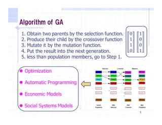
![Discrete Model
7
when we let 𝑝 𝑥T
𝑥, 𝑢 = 𝑢 𝑥T
𝑥
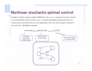
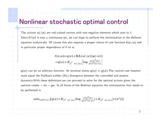
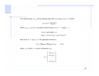
The bellman function of υ 𝑥 can write as
υ 𝑥 = min
V∈𝒰 X
{ℓ 𝑖, 𝑢 + EX]~_ ' 𝑥, 𝑢 𝜐(𝑥T
) }
optimal action will be
𝑢∗ 𝑥T 𝑥 =
𝑝 𝑥T 𝑥 𝓏 𝑥T
𝒢 𝓏 𝑥
𝓏 𝑥 = exp −𝑞 𝑥 𝒢 𝓏 𝑧 𝓏 = 𝑄𝑃𝓏
action cost of
current state
the value function
of next state](https://image.slidesharecdn.com/a4b6dc56-df6b-47cd-8e56-e6c8ac401da6-151117091452-lva1-app6891/85/slide-7-320.jpg)
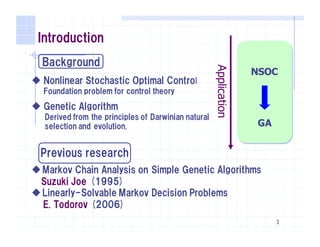
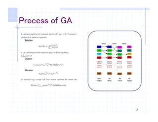
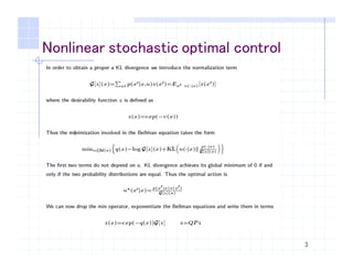
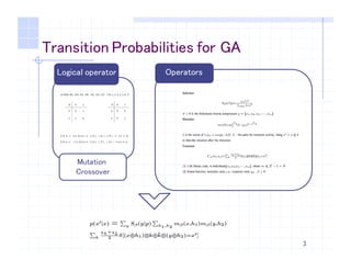
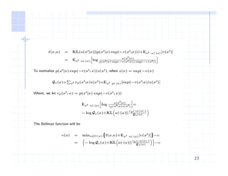
![Application of NSOC for GA
Transition probability of GA
Selection
𝑆j 𝑥T
𝑝 =
𝑓 𝑥T j
∑ 𝑓 𝑥 j
X∈_
Crossover𝐶X] 𝑥l, 𝑥m = ∑
nopnqo
6r 𝛿 𝑥l ⊗ 𝑘 ⊕ 𝑘w ⊗ 𝑥m = 𝑥T
Mutation
8
𝑚j ℎ = 𝜇j
{|}
(1 − 𝜇j)~•{|}
β ∶ Blotzman invese T
𝜇j = ϵ𝑒𝑥𝑝 −𝜆𝛽
ℎ mutation mask
𝑘 Crossover mask
𝑝 𝑥T 𝑥 = • 𝑆j 𝑦 𝑝
•
• 𝑚j 𝑥,ℎ{ 𝑚j(𝑦,ℎ6
}•,}‘
)
𝐶X] 𝑥l, 𝑥m •
𝜒r + 𝜒̅r
2
r
𝛿 (𝑥 ⊕ ℎ{)⊗ 𝑘 ⊕ 𝑘w ⊗ (𝑦 ⊕ ℎ6 = 𝑥T](https://image.slidesharecdn.com/a4b6dc56-df6b-47cd-8e56-e6c8ac401da6-151117091452-lva1-app6891/85/slide-8-320.jpg)
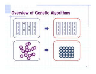
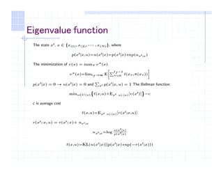
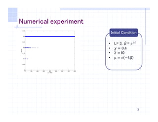
![Describe GA by NSC
let 𝑝 𝑥T 𝑥, 𝑢 = 𝑢 𝑥T 𝑥 = 𝑝 𝑥T 𝑥 𝑒𝑥𝑝 𝑢X];X
we can get eigenvalue function is
9
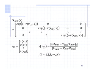
λ𝑧— = 𝒫 𝒩𝒩 𝑥 ℛ 𝒩𝒩 𝑥 𝑧 𝒩 (∀𝒙)
𝒫 𝒩𝒩(𝑥) =
𝑝 𝑥({) 𝑥 𝑝 𝑥(6) 𝑥 ⋯ 𝑝 𝑥(—) 𝑥
𝑝 𝑥({) 𝑥 𝑝 𝑥(6) 𝑥 ⋯ 𝑝 𝑥(—) 𝑥
⋮ ⋮ ⋱ ⋮
𝑝 𝑥({) 𝑥 𝑝 𝑥(6) 𝑥 ⋯ 𝑝 𝑥(—) 𝑥
0
0
0
0
0
1
0
1
1
1
0
0
1
0
1
1
1
0
0
1
0
1
1
1](https://image.slidesharecdn.com/a4b6dc56-df6b-47cd-8e56-e6c8ac401da6-151117091452-lva1-app6891/85/slide-9-320.jpg)
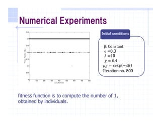
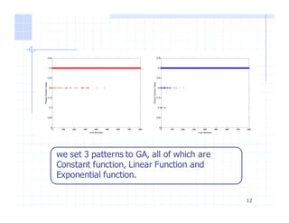
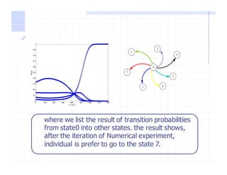
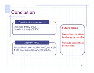

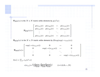

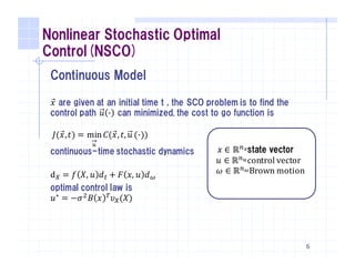
This document discusses applying nonlinear stochastic optimal control (NSOC) theory to genetic algorithms (GA). It provides an overview of GA and NSOC, describes modeling GA as a discrete-time controlled Markov process within the NSOC framework, and presents the results of a numerical experiment applying the NSOC-described GA to optimization problems. The experiment shows the transition probabilities between states after 800 iterations, indicating individuals prefer moving to state 7. The document concludes by noting future work could improve the fitness function and computation speed when applying NSOC to GA.