mechanical

1. MEEN 5326
Project #1
Modeling and Simulation of a Second Order Mechanical System
Due Date
The project is due on Tuesday Nov. 27, 2012. Please submit the project through the
Blackboard.
Report
A formal report is required describing your work including introduction, analytical
model, theoretical analysis, numerical approach, results, discussion, conclusion and
appendix. A sample report template is included in project folder. In the template, the
Table of Contents is automatically linked to the titles of each session. What you need to
do is right click on the Table of Contents and choose field updates and then update entire
table.
Objective
The intent of this project is 1) to develop models of second order system in MATLAB
and verified by analytical solution to address the response of a simple single degree of
freedom mechanical mass, spring, dashpot system due to initial conditions of
displacement and velocity; 2) to identify the system as underdamped, critical-damped,
overdamped and their corresponding response, 3) to apply the superposition principal to
the find the system response with both initial condition and input force applied, 4) to find
the transit response specification of a second order system.
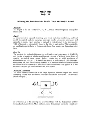
Model for Evaluation
The model used for evaluation is the single degree of freedom lumped mass model
defined by second order differential equation with constant coefficients. This model is
shown in Figure 1.
m is the mass, c is the damping and k is the stiffness with the displacement and the
forcing function, as shown. Mass, stiffness, initial displacement and initial velocity are

2. defined randomly by executing the Matlab script file (proj_parameter.m) in our class
folder. (Note: run the program twice, and use the data from the second run.)
Analytical Analysis for the Initial Conditions Problem
1. Derive the equation of motion describing this system. Here we assume that no external
forces are applied, that is f(t) = 0.
2. Assume the system is critical damped and no external forces are applied. Find the
damping coefficient c.
3. Assume the system is overdamped, and the damping ratio is 1.4. Also no external
forces are applied. Find the damping coefficient c. Derive the mathematical expression of
the displacement as a function of time with the given initial conditions. Plot your result.
4. Assume the system is underdamped, and the damping ratio is 0.5. Also no external
forces are applied. Find the corresponding damping coefficient c. Identify the system
parameters such as the natural frequency and damped frequency. Derive the mathematical
expression of the displacement as a function of time with the given initial condition. Plot
your result.
Analytical Analysis for the input force and Initial Conditions Problem
5. For the underdamped system in Problem 4, no initial conditions are applied. Input
force is a step function of 1.5 N. Derive the mathematical expression of the displacement
as a function of time. Plot your result.
6. For the underdamped system in Problem 4, same initial conditions are applied, and a
unit step function of 1.5 N is also applied as well. Derive the mathematical expression of
the displacement as a function of time. Plot your result.
MATLAB Solution the Initial Conditions Problem
7. For the above three systems, develop the MATLAB LTI commands in a script file to
describe a single degree of freedom mechanical mass, spring, dashpot system due to
initial conditions of displacement and velocity. The script should be commented and
provide the commands for graphical plotting all the three output signals in one figure.
Check how the damping ratio affects the system response. Compare the plots with your
analytical solution. (The MATLAB script file must be included.)
8. For the problems 4, 5, 6, develop the MATLAB LTI commands in a script file to find
the time response, respectively. Plot the three responses in the same figure, and discuss
the relationship among these plots.
Simulink Solution for the Forced Excitation
11. Develop a SIMULINK model to describe a single degree of freedom mechanical
mass, spring, dashpot system due to an external force and initial conditions (problems 6).
The model should be commented and should include graphical plotting of the output
signals. Assume the force excitation is a unit step with initial values same as the previous
work. Find the time responses of the underdamped system. (The SIMULINK file must be
included in Appendix.)

3. Specifications of the Unit Step Input
12. For the underdamped system in Problem 4, no initial conditions are applied. Input
force is a step function of 1.5 N. Find the rise time, peak time, settling time, and
maximum overshoot, analytically.
13. For the problem 12, develop the MATLAB LTI commands in a script file to find rise
time, peak time, settling time, and maximum overshoot, analytically. Compare the results
with your analytical solution in Problem 12. (The MATLAB script file must be included
in Appendix.)
SIMULINK Help
The following file is instructions of SIMULINK block diagram for a second order
system. You do not have to use the method provided here when you build a SIMULINK
model.