Tamil Call Girls Bhayandar WhatsApp +91-9930687706, Best Service
1 d heat conduction
1. 5.1
ONE-DIMENSIONAL, STEADY-STATE HEAT CONDUCTION
Essay 5
5.1 Planar Geometries
In basic courses in heat transfer, the treatment of conduction is confined to one-dimensional heat
flow. By definition, one-dimensional conduction is confined to heat flow in one coordinate
direction. An example of one-dimensional conduction can be seen by making reference to Fig.
3.3. To place the theory of one-dimensional conduction on a firm basis, the
simple slab depicted in Fig. 3.3 will be revisited and the appropriate solution
for both the temperature variation across the thickness of the slab and the rate
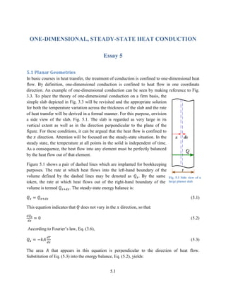
of heat transfer will be derived in a formal manner. For this purpose, envision
a side view of the slab, Fig. 5.1. The slab is regarded as very large in its
vertical extent as well as in the direction perpendicular to the plane of the
figure. For these conditions, it can be argued that the heat flow is confined to
the direction. Attention will be focused on the steady-state situation. In the
steady state, the temperature at all points in the solid is independent of time.
As a consequence, the heat flow into any element must be perfectly balanced
by the heat flow out of that element.
Figure 5.1 shows a pair of dashed lines which are implanted for bookkeeping
purposes. The rate at which heat flows into the left-hand boundary of the
volume defined by the dashed lines may be denoted as . By the same
token, the rate at which heat flows out of the right-hand boundary of the
volume is termed . The steady-state energy balance is:
(5.1)
This equation indicates that does not vary in the direction, so that:
(5.2)
According to Fourier’s law, Eq. (3.6),
(5.3)
The area that appears in this equation is perpendicular to the direction of heat flow.
Substitution of Eq. (5.3) into the energy balance, Eq. (5.2), yields:
Fig. 5.1 Side view of a
large planar slab
2. 5.2
(5.4)
For a plane slab, the area A does not depend upon x. The thermal conductivity may be x-
dependent, but that dependence will not be considered here. Instead, a mean conductivity equal
to:
(5.5)
is used in Eq. (5.4). Since and are independent of , Eq. (5.4) reduces to:
(5.6)
It is well known from freshman calculus that when the derivative of any quantity is zero, that
quantity must be a constant, so that:
(5.7)
Further integration yields:
(5.8)
The constants of integration, and , are found by the application of the boundary conditions
that and . The application of these conditions leads to the
solution:
(5.9)
If this solution is plotted on a graph of versus , there results:
Fig. 5.2 Temperature distribution for one-dimensional heat transfer across a plane slab
It can be seen from the figure that the temperature decreases linearly between the two end-point
temperatures and . This straight-line variation is valid only for a constant value of the
thermal conductivity.
3. 5.3
The rate of heat transfer across the slab can be obtained by applying Fourier’s law to the
temperature solution given by Eq. (5.9). The substitution of Eq. (5.9) into Eq. (5.3) yields:
(5.10)
The execution of the differentiation yields:
(5.11)
This equation can be re-written as:
(5.12)
where is the thermal resistance for one-dimensional heat transfer in a planar slab. The equation
for is:
(5.13)
which verifies Eq. (3.3).
5.2 Cylindrical Geometries
The approach illustrated in the previous section for the analysis of the planar geometries also
applies to cylindrical geometries provided that account is taken of the change of the cross-
sectional area that is encountered by the radial heat flow. To illustrate this point, reference
maybe made to Fig. 5.3. In the (a) part of the figure, a hollow-bore tube of finite length is
(a) (b)
Fig. 5. 3 Hollow bore cylindrical tube. (a) Three-dimensional; (b) Cross-sectional view for analysis
pictured. The tube has an inner radius and an outer radius . This nomenclature, shown in
the (b) part of the figure, is enhanced by the control volume outlined in red. The inner and outer
radii of the control volume are, respectively, and .
4. 5.4
Let the temperature at the surface of the bore of the tube be , and the temperature at the
outside surface of the tube be . These temperatures create a radially-outward heat flow . In
the steady state, is independent of the radial position. If were to vary with , the temperature
would necessarily vary with time. At any moment of time, let the magnitude of the heat
flow that is entering the control volume at the radius . By the same token, let
represent the heat flow that is leaving the control volume at a radius . In the steady state,
(5.14)
or,
(5.15)
Next, the radial heat flow is expressible by means of Fourier’s Law as:
(5.16)
The area is illustrated in Fig. 5.4. The magnitude of is equal to .
Fig. 5. 4 The area A(r) normal to the direction of radial heat flow
Introduction of the expression for into Eq. (5.16) and the substitution of the resulting
equation for into the energy-balance equation, Eq. (5.15), yields:
(5.17)
If can be regarded as a constant, or can be replaced by an average value as in Eq. (5.5), Eq.
(5.17) becomes:
(5.18)
By inspection,
(5.19)
5. 5.5
and,
(5.20)
The integration of this equation yields,
(5.21)
The integration constants and are determined by applying the boundary conditions that
and . The end result of this step is:
(5.22)
The temperature distribution represented by Eq. (5.22) is plotted in Fig. 5.5. It can be seen from
the figure that the distribution departs from the straight line that represents the temperature
variation in a planar one-dimensional geometry. The slope of the distribution for the cylindrical
case is greatest near the inside radius and decreases as the outer radius is approached.
Fig. 5. 5 Temperature distribution across the thickness of a cylindrical annulus
The rate of heat transfer passing through the cylindrical annulus can be obtained by making
use of Eq. (5.16) and the temperature distribution from Eq. (5.22). When the indicated operations
are performed, there is obtained:
(5.23)
From this, it follows that the thermal resistance of a cylindrical annulus is:
(5.24)