2. Annals of Nuclear Energy 195 (2024) 110181
2
2019). It encodes prior information from differential equations rather
than existing data into the training model, which is very different from
the traditional data-driven deep learning method, and can effectively
reduce the computational cost.
Compared with traditional numerical methods, PINN has many
unique advantages, some of which are a natural fit for solving NTE. As a
mesh-free method, PINN randomly selects discrete points within the
computational region. This approach is insensitive to the dimension of
the computational region and can partially avoid the curse of dimen
sionality. Additionally, PINN is well adapted to complex geometry since
there is no need to construct a high-quality mesh and only requires
randomly selecting points in the calculation region. Furthermore, PINN
provides a continuous solution, allowing for the solution value to be
obtained at any point in the calculation region and not limited to pre-set
discrete points. This feature effectively reduces ray effects of NTE so
lutions caused by solid angular discretization, as demonstrated in Sec
tion 3.4.
Previous work has been conducted to apply PINN to solve problems
in neutron calculations. Elhareef introduced PINN to solve neutron
diffusion problems and achieved solutions for fixed source problems and
k-eigenvalue problems (Elhareef and Wu, 2022). Schiassi applied PINN
for solving point kinetics equations (Schiassi et al., 2022). Wang pro
posed cPINN, which places different PINNs in each subregion to solve
multi-region neutron diffusion problems (Wang et al., 2022). In our
earlier work (Xie et al., 2021), PINN was improved and enhanced by
introducing boundary conditions (BCs) into the trial function, resulting
in an improvement in calculation accuracy by hundreds of times in
neutron diffusion examples. Building on this previous work, this paper
extends BDPINN to neutron transport calculations. The main contribu
tions of this work are as follows: (1) A novel numerical algorithm,
BDPINN is applied to solve NTE, and its accuracy is proved; (2) A third-
order tensor is introduced to transform the integral term in NTE to avoid
expression swell; (3) Some original forms of trial function are proposed
for common boundary conditions in NTE; (4) The feasibility of BDPINN
to provide a universal solution is discussed and proved; (5) The rear
rangement of training set is proposed to reduce the error near the
interface; (6) The reason of ray effect is discussed and a simple but
effective technique to reduce ray effect on BDPINN is proposed; (7) The
area decomposition and multi-group iteration are successfully used in
BDPINN to solve multi-group and complex area problems.
The rest of this paper is organized as follows. In Section 2, the NTE,
the main idea of BDPINN, some construction approaches of trial function
and some techniques of BDPINN are introduced in order. Four cases are
tested to prove the superiority of BDPINN in Section 3. The main con
clusions of this paper are summarized in Section 4.
2. Methodology
The NTE is very different from neutron diffusion equation (NDE),
thus the BDPINN used in NTE should be different from that of NDE (Xie
et al., 2021). First, the NTE is an integro-differential equation that in
cludes some multiple integrals with respect to the angle and energy.
Discretization about these multiple integrals leads to expression swell.
Second, the non-smoothness of the NTE at the physical interface leads to
additional errors in the BDPINN. Finally, the discretization of the angle
variable in the NTE can lead to ray effects, which reduce the accuracy of
the calculated results. In this work, monoenergetic NTE is focused and
three techniques are proposed in order to solve the above three problems
and improve BDPINN: third-order tensor transformation, rearrangement
of training set and result reconstruction in high order. In this section,
NTE and BDPINN are briefly introduced, then a systematic construction
process of trial function is given, and finally the three techniques are
presented in detail.
2.1. Neutron transport equation
The multi-group NTE can be described as:
∂ψg
∂t
+ Ω
→
⋅∇ r
→ψg + Σt,gψg = Qg
(
ψg
)
(1)
where ψg( r
→, Ω
→
, t) is the neutron angular flux with the dependency of
space variable r
→ = (x, y, z) ∈ Ω⊂R3
, motion direction variable Ω
→
=
(μ, η, ξ) ∈ S = S2
and time variable t ∈ [0, T] in energy group g; Σt,g( r
→) is
the macroscopic total cross section in energy group g; Qg(ψ) is the source
term including the scattering term, the fission term and the external
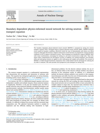
source term in energy group g. The direction variable Ω
→
and its com
ponents μ, η and ξ in unit sphere is illustrated with Fig. 1. μ, η and ξ are
projections of Ω
→
on the ×,y and z axes, respectively.
In this work, scattering is considered to be isotropic, and the fission
term is ignored. Therefore, the source term can be described as:
Qg
(
ψg
)
=
Qext,g +
∑G
g′=1Σs,g′→gϕg′
4π
, ϕg =
∫
S
ψg dΩ
→
(2)
where Qext,g is the external source term independent of ψg; Σs,g′→g( r
→) is
the scattering cross section; ϕg is the zeroth angular moment of ψg,
representing the neutron scalar flux; G is the number of energy groups.
2.2. Neural network
BDPINN is a multi-layer feed-forward neural network, which can be
composed of elementary functions. It passes the input to the output
through several hidden layers consisting of nonlinear mappings. A feed-
forward neural network with n + 1 layers can be described as:
NN(I, p
→) = fa(fa(⋯fa(fa(IW1 + B1)W2 + B2)Wn− 1⋯ + Bn− 1)Wn + Bn) = O
(3)
where NN is the neural network function; I is the input array; fa is the
activation function; W with subscript is the weight matrix; B with
subscript is the bias matrix; p
→ is tuning parameters representing the
Fig. 1. Direction variable in the unit circle.
Y. Xie et al.
3. Annals of Nuclear Energy 195 (2024) 110181
3
ensemble of all weight and bias matrix and O is the output array. Popular
activation function used in the machine learning include the sigmoid
function, the hyperbolic tangent function and the ReLU function. Ac
cording our early work (Xie et al., 2021), the hyperbolic tangent func
tion has a better performance and is therefore chosen as the activation
function for all four cases in this work.
2.3. BDPINN for monoenergetic NTE
The calculation of multi-group NTE by BDPINN is based on the
calculation of monoenergetic NTE. The calculation of multi-groups is
mentioned in Section 2.9. Here, the calculation of monoenergetic NTE is
introduced first.
BDPINN transforms monoenergetic NTE into an optimization prob
lem of a loss function containing a neural network with tunning
parameter p
→, which consists of weights and biases of neural network. A
schematic diagram of BDPINN is shown in Fig. 2. It begins with the
construction of neural network. r
→, Ω
→
and t form the input array I of
neural network. The input array is transferred through multiple hidden
layers. The output array is then available.
The next step is to define a trial function, which is an approximation
of the NTE solution and is defined differently. In classical PINN, the trial
function is directly defined by the neural network, which can be
described as:
ψ
(
r
→, Ω
→
, t
)
= NN
(
r
→, Ω
→
, t, p
→
)
(4)
In BDPINN, the trial function includes the constraints of BCs and can
be described as:
ψ
(
r
→, Ω
→
, t, p
→
)
= A
(
r
→, Ω
→
, t
)
+ B
(
r
→, Ω
→
, t, NN
(
r
→, Ω
→
, t, p
→
))
(5)
where A( r
→, Ω
→
, t) is a function that fits all BCs and B( r
→, Ω
→
, t, NN) is a
function that has no contribution to BCs. For example, for constant
Dirichlet BC, term A should be equal to the boundary constant and B
should be zero on this boundary. Through this construction, the trial
function can perfectly and naturally satisfy all BCs. Obviously, the ex
pressions of A and B depend on BCs. This is a tricky problem in BDPINN.
A systematic construction process is detailed in Section 2.4.
The final step is called equation-driven training. With the help of
automatic differentiation, the derivatives and source information are
obtained to form the loss function, which is defined differently in
BDPINN and classical PINN. In classical PINN, the constraints of BCs are
absent in trial function of Eq. (4). Thus, both the governing equation and
all BCs are required in loss function to approach the NTE solution. In
BDPINN, only the governing equation is introduced in loss function,
which can be described as:
loss =
∂ψ
∂t
+ Ω
→
⋅∇ r
→ψ + Σtψ − Q(ψ) (6)
The loss function inherits the form of NTE, which means that when
the loss equals to zero, the boundary dependent trial function is perfectly
satisfied NTE and is therefore the solution of NTE. At this point, the NTE
is transformed into an optimization problem of the loss function with
tunning parameter p
→, space variable r
→, direction variable Ω
→
,and time
variable t. If the optimization of the loss function is successful, the
boundary dependent trial function that basically satisfies NTE is ob
tained and can be regarded as an approximate solution of NTE. Since the
loss function is defined in the entire computational region, optimizing
the loss function to zero means that it is always zero in the entire
computational region, which is a very difficult requirement in numerical
computation. Therefore, it is common practice to weaken this require
ment to the point that the loss function tends to zero at some discrete
points in the computational region. The set formed by these discrete
points is called training set and its size is denoted by Ntrain. The chosen of
these discrete points is random in both space and velocity. The velocities
of different discrete points are different from each other.
The loss function in BDPINN for NTE on training set can be defined
by L2
norm:
Fig. 2. Schematic diagram of BDPINN for NTE.
Y. Xie et al.
4. Annals of Nuclear Energy 195 (2024) 110181
4
where variables with subscript i represent the points in the training set.
As Eq. (7) shown, the loss function on training set depends only on the
tunning parameter p
→. Adjusting the tunning parameter to make the loss
as close to 0 as possible, this is the meaning of training. In machine
learning, the optimization of loss function is solved by first-order
gradient descent methods, such as Adam (Kingma and Ba, 2014), or
second-order gradient descent methods, such as LBFGS (Liu and Noce
dal, 1989), which is chosen in this work.
2.4. Systematic construction process of trial functions in BDPINN
The BDPINN requires a specified trial function to satisfy a specified
set of BCs (i.e., a combination of BCs). Therefore, the form of trial
function varies according to the BCs of the computational domain. It is
worth noting that the construction of trial function is independent of the
governing equation, therefore, the constructed trial functions can also
be applied to solve other physical equations. Although designing the
trial function is an empirical and skillful work, for Dirichlet and sym
metric BCs commonly used in engineering applications of NTE, we
propose a systematic process to simplify this design. This process can be
simply divided into three steps: First, if there is symmetry, virtually
recover the entire computational region by mirror replication along
symmetric boundaries. Second, design some trial functions satisfying a
single Dirichlet BC respectively. Finally, combine all trial functions
corresponding to different BCs to form a trial function satisfying a
combination of multiple BCs. Obviously, if there is only one Dirichlet BC,
the first and final step can be skipped. This is what happens in Case 1 and
4.
In the first step, we need to mirror replication the computational
region to remove symmetric BCs. In practical calculation, the symmetry
BC is sometimes applied to the entire calculation area based on the
symmetry of the solution, so as to reduce the computation cost. For a
symmetry BC, all we need to do is reverse this process to recover the
computational region and remove the symmetric BC. After the reversal,
new Dirichlet BCs sometimes appear, as in Case 2 and 3. However, the
most important trick in this step is that the recovered computational
region is virtual. The additional computational region created by mirror
replication is called the virtual computational region Ωv
where no
discrete points will be chosen. The selection of discrete points only oc
curs on the original computational region before the symmetry inver
sion, which is called the real computational region. With this trick, the
increase of computational cost is avoided while eliminating the sym
metric BC.
In the second step, we need to design a trial function that satisfies a
single Dirichlet BC. A single Dirichlet BC and a trial function satisfying
this BC can be described as:
∀ r
→ ∈ Γ⊂Ω, ψ
(
r
→, Ω
→
, t
)
= g
(
r
→, Ω
→
, t
)
(8)
and
ψ
(
r
→, Ω
→
, t, p
→
)
= A
(
r
→, Ω
→
, t
)
+ C
(
r
→, Ω
→
, t
)
NN
(
r
→, Ω
→
, t, p
→
)
(9)
where the Γ is part of the computational region boundary and g is a
known function. The trial function Eq. (9) is different from its original
form Eq. (5), because here it only needs satisfy a single Dirichlet BC. The
requirements for term A and term C can be detailed as:
{
A
(
r
→, Ω
→
, t
)
= g
(
r
→, Ω
→
, t
)
B
(
r
→, Ω
→
, t
)
= 0
, ∀ r
→ ∈ Γ (10)
Some trial function designed by Eq. (9) are detailed in the four cases
used in this work.
In the final step, a trial function satisfying a combination of multiple
BCs should be determined. Fortunately, in NTE, the vacuum BC is the
most common Dirichlet BC, which requires the function value to be 0.
Then the term A in Eq. (9) becomes 0. At this time, it is only necessary to
multiply the terms C corresponding to different vacuum BCs to obtain a
trial function that satisfies multiple vacuum BCs. Some trial functions
obtained in this way are shown in detail in Case 2 and 3 of Section 3.
2.5. Third-order tensor transforming quadrature set
The technique presented in this subsection aims to avoid the
expression swell caused by the discretization of the double integral in
NTE. This subsection begins with a brief introduction to the expression
swell problem, and then elaborates on the third-order tensor trans
formation used to solve this problem.
NTE is an integro-differential equation. The integral term in NTE is
discretized by a quadrature set, which can be described as:
ϕ( r
→, t) =
∫
S
ψ
(
r
→, Ω
→
, t
)
dΩ
→
≈
∑
j
wjψ
(
r
→, Ω
→
j, t
)
(11)
where w with subscript is the quadrature weight and v
→ with subscript is
the quadrature points. However, when computing multiple integrals, the
number of terms in the quadrature set Nint swells with the quadrature
order increasing. For example, in the discrete ordinate method, Nint is 40
for S8, 144 for S16, and 312 for S24. If S24 is used in losstrain with Ntrain
equals to 10,000 to discrete integral term, the number of terms in losstrain
will be 3,150,000. Such a huge number of terms is an enormous burden
even for automatic differentiation technique. Therefore, in the field of
deep learning, transforming the input into a matrix is usually used to
deform losstrain.
We denote Strain = {( r
→
i, Ω
→
i, t)
⃒
⃒
⃒
⃒ r
→
i ∈ Ω, Ω
→
∈ S, t ∈ [0, T]} for 1⩽i⩽
Ntrain as the training set. The training set is wrapped into the input
training array Itrain, which is a second-order tensor with shape Ntrain × 7,
which can be described as:
Itrain =
⎡
⎢
⎢
⎢
⎢
⎢
⎣
r
→
1 = (x1, y1, z1) Ω
→
1 = (μ1, η1, ξ1) t1
⋮
r
→
i = (xi, yi, zi) Ω
→
i = (μi, ηi, ξi) ti
⋮
r
→
Ntrain =
(
xNtrain , yNtrain , zNtrain
)
Ω
→
Ntrain =
(
μNtrain
, ηNtrain
, ξNtrain
)
tNtrain
⎤
⎥
⎥
⎥
⎥
⎥
⎦
(12)
According to the rules of matrix operation, the neural network NN
receiving the matrix Itrain as input provides a matrix output, which is of
shape Ntrain × 1 and can be described as:
losstrain( p
→) =
∑
Ntrain
i=1
⎛
⎜
⎜
⎝
∂ψ
∂t
(
r
→
i, Ω
→
i, ti, p
→
)
+ Ω
→
i⋅∇ r
→ψ
(
r
→
i, Ω
→
i, ti, p
→
)
+ Σt( r
→)ψ
(
r
→
i, Ω
→
i, ti, p
→
)
− Q
(
ψ
(
r
→
i, Ω
→
i, ti, p
→
))
⎞
⎟
⎟
⎟
⎠
2
(7)
Y. Xie et al.
5. Annals of Nuclear Energy 195 (2024) 110181
5
NN(Itrain, p
→) =
⎡
⎢
⎢
⎢
⎢
⎢
⎣
NN
(
r
→
1, Ω
→
1, t1, p
→
)
⋮
NN
(
r
→
i, Ω
→
i, ti, p
→
)
⋮
NN
(
r
→
Ntrain
, Ω
→
Ntrain
, tNtrain
, p
→
)
⎤
⎥
⎥
⎥
⎥
⎥
⎦
(13)
According to Eq. (2) and Eq. (5), related A(Itrain), B(Itrain,NN), ψt(Itrain,
p
→) and Q(ψt(Itrain, p
→)) are of shape Ntrain × 1 and are defined as follows:
A(Itrain) =
⎡
⎢
⎢
⎢
⎢
⎢
⎣
A
(
r
→
1, Ω
→
1, t1
)
⋮
A
(
r
→
i, Ω
→
i, ti
)
⋮
A
(
r
→
Ntrain , Ω
→
Ntrain , tNtrain
)
⎤
⎥
⎥
⎥
⎥
⎥
⎦
(14)
B(Itrain, NN) =
⎡
⎢
⎢
⎢
⎢
⎢
⎢
⎣
B
(
r
→
1, Ω
→
1, t1, NN
(
r
→
1, Ω
→
1, t1, p
→
))
⋮
B
(
r
→
i, Ω
→
i, ti, NN
(
r
→
i, Ω
→
i, ti, p
→
))
⋮
B
(
r
→
Ntrain
, Ω
→
Ntrain
, tNtrain
, NN
(
r
→
Ntrain
, Ω
→
Ntrain
, tNtrain
, p
→
))
⎤
⎥
⎥
⎥
⎥
⎥
⎥
⎦
(15)
ψ(Itrain, p
→) =
⎡
⎢
⎢
⎢
⎢
⎢
⎣
ψ
(
r
→
1, Ω
→
1, t1, p
→
)
⋮
ψ
(
r
→
i, Ω
→
i, ti, p
→
)
⋮
ψ
(
r
→
Ntrain , Ω
→
Ntrain , tNtrain , p
→
)
⎤
⎥
⎥
⎥
⎥
⎥
⎦
(16)
and
Q(ψ(Itrain, p
→)) =
⎡
⎢
⎢
⎢
⎢
⎢
⎢
⎣
Q
(
ψ
(
r
→
1, Ω
→
1, t1, p
→
))
⋮
Q
(
ψ
(
r
→
i, Ω
→
i, ti, p
→
))
⋮
Q
(
ψ
(
r
→
Ntrain , Ω
→
Ntrain , tNtrain , p
→
))
⎤
⎥
⎥
⎥
⎥
⎥
⎥
⎦
=
⎡
⎢
⎢
⎢
⎢
⎢
⎢
⎢
⎢
⎢
⎢
⎢
⎢
⎢
⎣
Qext
4π
+
Σs( r
→)
4π
∑
j
wjψ
(
r
→
1, Ω
→
j, t1, p
→
)
⋮
Qext
4π
+
Σs( r
→)
4π
∑
j
wjψ
(
r
→
i, Ω
→
j, ti, p
→
)
⋮
Qext
4π
+
Σs( r
→)
4π
∑
j
wjψ
(
r
→
Ntrain , Ω
→
j, tNtrain , p
→
)
⎤
⎥
⎥
⎥
⎥
⎥
⎥
⎥
⎥
⎥
⎥
⎥
⎥
⎥
⎦
(17)
By these matrix terms, the loss function in training set can be
rewritten as the form of matrix:
where MNtrain
is an all-ones matrix with shape 1 × Ntrain. We denote Nint
the number of quadrature set. By transforming the input into a matrix,
the number of terms in losstrain of eq. (7) is successfully reduced from
(Nint + 4) Ntrain to Nint + 4, where the number of four represents the
transient term, the convective term, absorption term and external source
term. But losstrain still suffers from the expression swell caused by Nint.
Therefore, the third-order tensor is introduced to redeform the losstrain
and avoid this swell problem.
We denote Sint = {(wj, μj, ηj, ξj)
⃒
⃒
⃒wj ∈ R, (μj, ηj, ξj) ∈ S} for 1⩽j⩽Nint as
the quadrature set. The third-order input training array I
(3)
train is formed by
Strain and Sint, and is described as:
I(3)
train =
⎡
⎢
⎢
⎢
⎢
⎢
⎢
⎢
⎢
⎢
⎢
⎢
⎢
⎢
⎢
⎢
⎢
⎢
⎢
⎢
⎢
⎢
⎢
⎢
⎢
⎢
⎢
⎢
⎢
⎣
⎡
⎢
⎢
⎢
⎢
⎢
⎢
⎢
⎢
⎢
⎣
r
→
1 = (x1, y1, z1) Ω
→
1 = (μ1, η1, ξ1) t1
⋮
r
→
1 = (x1, y1, z1) Ω
→
j =
(
μj, ηj, ξj
)
t1
⋮
r
→
1 = (x1, y1, z1) Ω
→
Nint
=
(
μNint
, ηNint
, ξNint
)
t1
⎤
⎥
⎥
⎥
⎥
⎥
⎥
⎥
⎥
⎥
⎦
⋮
⎡
⎢
⎢
⎢
⎢
⎢
⎢
⎢
⎢
⎢
⎣
r
→
i = (xi, yi, zi) Ω
→
1 = (μ1, η1, ξ1) ti
⋮
r
→
i = (xi, yi, zi) Ω
→
j =
(
μj, ηj, ξj
)
ti
⋮
r
→
i = (xi, yi, zi) Ω
→
Nint =
(
μNint
, ηNint
, ξNint
)
ti
⎤
⎥
⎥
⎥
⎥
⎥
⎥
⎥
⎥
⎥
⎦
⋮
⎡
⎢
⎢
⎢
⎢
⎢
⎢
⎢
⎢
⎢
⎣
r
→
Ntrain
=
(
xNtrain
, yNtrain
, zNtrain
)
Ω
→
1 = (μ1, η1, ξ1) tNtrain
⋮
r
→
Ntrain
=
(
xNtrain
, yNtrain
, zNtrain
)
Ω
→
j =
(
μj, ηj, ξj
)
tNtrain
⋮
r
→
Ntrain
=
(
xNtrain
, yNtrain
, zNtrain
)
Ω
→
Nint
=
(
μNint
, ηNint
, ξNint
)
tNtrain
⎤
⎥
⎥
⎥
⎥
⎥
⎥
⎥
⎥
⎥
⎦
⎤
⎥
⎥
⎥
⎥
⎥
⎥
⎥
⎥
⎥
⎥
⎥
⎥
⎥
⎥
⎥
⎥
⎥
⎥
⎥
⎥
⎥
⎥
⎥
⎥
⎥
⎥
⎥
⎥
⎦
(19)
I
(3)
train is of shape Ntrain × Nint × 7 and can be seen as a stack of Ntrain
matrices with shape of Nint × 7. According to the rules of array opera
tion, the neural network NN receiving the third-order tensor I
(3)
train as
input provides a matrix output, which is of shape Ntrain × Nint and can be
described as:
losstrain( p
→) = MNtrain
⎡
⎢
⎣
∂ψ
∂t
(Itrain, p
→) + Ω
→
train⋅∇ r
→ψ(Itrain, p
→) + Σt( r
→)ψ(Itrain, p
→) − Q(ψ(Itrain, p
→))
⎤
⎥
⎦ (18)
Y. Xie et al.
6. Annals of Nuclear Energy 195 (2024) 110181
6
The corresponding ψt(I
(3)
train, p
→) is of shape Ntrain × Nint and can be
defined as:
It is worth noting that I
(3)
train and ψ(I
(3)
train, p
→) are used to make the
quadrature set into a matrix, and the losstrain is still defined on the
training set. The integral weight array Wint is defined as:
Wint =
⎡
⎢
⎢
⎢
⎢
⎢
⎢
⎢
⎢
⎢
⎣
w1
⋮
wj
⋮
wNint
⎤
⎥
⎥
⎥
⎥
⎥
⎥
⎥
⎥
⎥
⎦
(22)
At this point, Q(ψ(Itrain, p
→)) can be rewritten as:
Q(ψ(Itrain, p
→)) =
Qext
4π
+
Σs( r
→)
4π
ψ
(
I(3)
train, p
→
)
× Wint (23)
The summation in Eq. (17) is converted into matrix products. Thus,
the number of terms in losstrain is reduced from Nint + 4 to 5 and the
expression swell caused by integral discretization is avoided. This
technique is applied in cases with scattering term, including Case 2, 3
and 4 of Section 3.
2.6. Rearrangement of training set
As a mesh-free method, BDPINN does not suffer from many re
strictions in selecting training set. In most BDPINN applications, the way
to select the training set points is randomly selecting the values of all
variables within the phase space simultaneously, including space vari
able r
→, direction variable Ω
→
and time variable t. However, this way does
not perform well on some cases with physical interfaces. The reason is
that the trial function based on the smooth neural network is smooth on
the physical interface, but the solution of NTE can only maintain con
tinuity but not smoothness on the physical interface. A reasonable so
lution is to increase the density of training points near the interface. But
it also increases the computational cost. A compromised solution is to
rearrange the training set without changing the size of the training set,
so as to increase the density of training points near the interface. Mao
et al. have tried this method in discontinuous interface (Mao et al.,
2020). Whereas in NTE, the particle density function is always contin
uous over the computational region and non-derivable on the physical
interface. In this work, the rearrangement of training set is proposed and
validated in cases with continuous but non-derivable interface,
including Case 1, 3 and 4.
2.7. Result reconstruction in high order
BDPINN provides a continuous solution. Although the loss function is
trained on the training set, the trial function is defined on the entire
computational region, which means that the particle density of any
point in the computational region at any time and in any direction can
be obtained.
The discretization of integral term in NTE brings inevitable error of
ray effect. Increasing the order of the quadrature set in the whole
calculation process can reduce the ray effect, but at the cost of increased
computational complexity. In this work, a simple technique, named
result reconstruction in high order, is proposed based on the continuity
of BDPINN solution, which has a magical influence on reducing the ray
Table 1
Summary of important parameters used in all four cases.
Number of
hidden layers
Number of
neurons in each
layer
Training
set size
Quadrature set for
training: type and
order
Case
1
2 256 1,200 Gauss-Legendre;
eight
Case
2
10 40 400 Gauss-Legendre;
eight
Case
3
12 100 19,964 Level-symmetric;
eight
Case
4
14 120 25,000 Level-symmetric;
eight
Case
5
12 512 6,400 Level-symmetric;
eight
NN
(
I
(3)
train, p
→
)
=
⎡
⎢
⎢
⎢
⎢
⎢
⎣
NN
(
r
→
1, Ω
→
1, t1, p
→
)
⋮
NN
(
r
→
i, Ω
→
1, ti, p
→
)
⋮
NN
(
r
→
Ntrain
, Ω
→
1, tNtrain
, p
→
)
⋯
⋱
⋯
⋱
⋯
NN
(
r
→
1, Ω
→
j, t1, p
→
)
⋮
NN
(
r
→
i, Ω
→
j, ti, p
→
)
⋮
NN
(
r
→
Ntrain , Ω
→
j, tNtrain , p
→
)
⋯
⋱
⋯
⋱
⋯
NN
(
r
→
1, Ω
→
Nint , t1, p
→
)
⋮
NN
(
r
→
i, Ω
→
Nint , ti, p
→
)
⋮
NN
(
r
→
Ntrain , Ω
→
Nint , tNtrain , p
→
)
⎤
⎥
⎥
⎥
⎥
⎥
⎦
(20)
ψ
(
I
(3)
train, p
→
)
=
⎡
⎢
⎢
⎢
⎢
⎢
⎣
ψ
(
r
→
1, Ω
→
1, t1, p
→
)
⋮
ψ
(
r
→
i, Ω
→
1, ti, p
→
)
⋮
ψ
(
r
→
Ntrain , Ω
→
1, tNtrain , p
→
)
⋯
⋱
⋯
⋱
⋯
ψ
(
r
→
1, Ω
→
j, t1, p
→
)
⋮
ψ
(
r
→
i, Ω
→
j, ti, p
→
)
⋮
ψ
(
r
→
Ntrain , Ω
→
j, tNtrain , p
→
)
⋯
⋱
⋯
⋱
⋯
ψ
(
r
→
1, Ω
→
Nint , t1, p
→
)
⋮
ψ
(
r
→
i, Ω
→
Nint , ti, p
→
)
⋮
ψ
(
r
→
Ntrain , Ω
→
Nint , tNtrain , p
→
)
⎤
⎥
⎥
⎥
⎥
⎥
⎦
(21)
Y. Xie et al.
7. Annals of Nuclear Energy 195 (2024) 110181
7
effect. Firstly, choose a low order quadrature set for the third-order
input training array I
(3)
train to optimize the loss function, then a trained
trial function continuous in both space and direction phase space will be
obtained. Secondly, use the trained trial function to calculated F with a
high order quadrature set, depending on the continuity of the trial
function. The technique of result reconstruction in high order requires
only a very small computational cost, but can greatly reduce the ray
effect, thereby achieving an increase in computational accuracy, which
is applied and validated in Case 4.
2.8. Area decomposition
For problems with complicated geometries, the effect of the rear
rangement of training set is not so significant. One possible solution is
area decomposition. This idea is inspired by Wang’s use of PINN to solve
multi-area neutron diffusion problems (Wang et al., 2022). But unlike
solving the neutron diffusion equation, the first-order derivative conti
nuity condition is not required for solving the NTE, only the value
continuity condition is required. This is because the NTE has only first-
order derivative terms but no second-order derivative terms. Therefore,
the loss function is given by:
loss =
∑
M
i=1
losstrain,i +
∑
P
i=1
lossinterface,i (24)
where M is the number of areas; P is the number of interfaces between
different areas; lossinterface,i represents the loss of value continuity con
dition on the interface i, which can be described by
lossinterface,i =
∑
Ninterface,i
j=1
(
ψm
(
r
→
j, Ω
→
j, tj, p
→
j
)
− ψn
(
r
→
j, Ω
→
j, tj, p
→
j
))2
(25)
where Ninterface,i is the number of points on the interface i; ψm and ψn
represent the neutron angular flux on both sides of the interface i.
2.9. Multi-group iteration
In the multi-group NTE, the scattering neutron source from other
energy groups is included. Therefore, the multi-group NTE is a coupled
system of integral–differential equations, which can be solved using
source iteration (Holloway and Akkurt, 2004). The implementation of
multi-group calculation can be briefly described as follows: with
initializing the scattering source of each energy group, the NTE of each
group is solved using the method in Section 2.3 one by one; after that,
the scattering source term is updated and the calculation for each group
is restart with updated scattering source; this iteration is repeated until
all energy groups converge.
3. Results and discussion
There are four cases in this work to study and explore the application
of BDPINN for NTE solving. The Case 1 and 2 investigate the application
of BDPINN on one-dimensional transport problems. The Case 3 and 4
Fig. 3. Geometry of Case 1 of a 1D neutron transport.
Fig. 4. Train set of Case 1.
Fig. 5. Comparison of BDPINN solution and BMS of Case 1.
Table 2
Summary of absolute error in Case 1.
Absolute error/10− 3
Maximum Average
BDPINN (dense) 21.3 6.93
BDPINN (no dense) 63.1 15.0
Y. Xie et al.
8. Annals of Nuclear Energy 195 (2024) 110181
8
investigate the application of BDPINN on two-dimensional transport
problem with rectangle and circle boundary, respectively. The Case 5
validates the application of BDPINN on multi-group transport problem
with multi area. The one-dimensional problems, whose phase space
dimension is two, are implemented on a single NVIDIA GeForce GTX
1660ti GPU card, while the two-dimensional problems, whose phase
space dimensional is four, are implemented on a single NVIDIA GeForce
RTX 3090 GPU card.
The neural network structure, training set size and quadrature set
used for all four cases are listed in Table 1.
3.1. Case 1: 1D transport problem with scattering
Case 1 is a one-dimensional mono-energy stationary neutron trans
port problem with scattering term. In this case, the NTE of Eq. (1) is
simplified to
μ
∂ψ
∂x
+ Σtψ =
Qext + Σsϕ
4π
(26)
where ψ(x, μ) is regarded as radiative intensity.
The Case 1 is modified from an eigenvalue problem (Larsen and
Yang, 2008), and the fission term is merged into the scattering term. The
geometry and parameters are presented in Fig. 3. The entire computa
tional region is divided into three regions with different scattering
terms. Two vacuum BCs are described as:
ψ(210, μ < 0) = 0 (27)
and
ψ(0, μ > 0) = 0 (28)
Two trial functions for BCs satisfying Eq. (27) and Eq. (28), respec
tively, can be described as:
ψ(x, μ) =
(
(210 − x)2
+ (|μ| + μ)
)
NN(x, μ, p
→) (29)
and
ψ(x, μ) =
(
x2
+ (|μ| − μ)
)
NN(x, μ, p
→) (30)
Comprehensively, a trial function satisfying both Eq. (27) and Eq. (28)
can be easily given by:
ψ(x, μ) =
(
(210 − x)2
+ (|μ| + μ)
)(
x2
+ (|μ| − μ)
)
NN(x, μ, p
→) (31)
The benchmark solution (BMS) is provided by finite element method
(FEM) with 300 elements and 301 nodes.
For this 1D transport problem, a two-dimensional computational
domain of {(x, μ)|(x, μ) ∈ [0, 210] × [ − 1, 1]} is used to choose random
training set. Since there are two interfaces in this case, the rearrange
ment of training set described in Section 2.6 is adopted. To reduce the
computational error around the interface x = 5 cm and x = 205 cm, 400
points are selected in each of the three intervals [0, 10], [10, 200] and
[200, 210], as shown in Fig. 4.
BDPINN with and without dense region are compared with BMS in
Fig. 5, which indicates that BDPINN can get an accurate result of 1D
NTE. The information of comparison is summarized in Table 2. The
Fig. 6. Geometry of Case 2 of a 1D neutron transport.
Fig. 7. Recovered geometry of Case 2.
Fig. 8. Comparison of BDPINN solution and BMS of Case 2.
Fig. 9. Geometry of Case 3 of a 2D neutron transport.
Y. Xie et al.
9. Annals of Nuclear Energy 195 (2024) 110181
9
rearrangement of training set can effectively improve the computational
accuracy of BDPINN, as shown in Fig. 5.
3.2. Case 2: 1D transport problem with symmetric boundary
Case 2 mainly aims to verify the reliability and accuracy of BDPINN
on 1D transport problem with scattering medium and special BCs.
Case 2 is a one-dimensional monoenergetic stationary neutron
transport problem with scattering term. In this case, the NTE of Eq. (1) is
simplified to:
μ
∂ψ
∂x
+ Σtψ =
Qext + Σsϕ
4π
(32)
where ψ(x, μ) is the neutron angular flux and ϕ is the neutron flux
defined as ϕ =
∫
Sψ dΩ
→
. The third-order tensor transforming quadrature
set described in Section 2.5 is introduced to calculate the integral term.
The geometry, parameters and BCs are presented in Fig. 6. All three
steps described in Section 2.4 need to be performed due to the existence
of the symmetric boundary. After applying mirror replication, a virtual
computational region Ωv
and a new vacuum BC are obtained, as shown
in Fig. 7. In the first step, the combination of one symmetric BC and one
vacuum BC are transformed into the combination of two vacuum BCs
described as
ψ(1, μ < 0) = 0 (33)
and
ψ( − 1, μ > 0) = 0 (34)
In the second step, two trial functions satisfying Eq. (33) and Eq.
(34), respectively, can be described as:
ψ(x, μ) =
(
(1 − x)2
+ (|μ| + μ)
)
NN(x, μ, p
→) (35)
and
ψ(x, μ) =
(
(1 + x)2
+ (|μ| − μ)
)
NN(x, μ, p
→) (36)
In the final step, a trial function satisfying both Eq. (33) and Eq. (34)
can be easily given by:
ψ(x, μ) =
(
(1 − x)2
+ (|μ| + μ)
)(
(1 + x)2
+ (|μ| − μ)
)
NN(x, μ, p
→) (37)
No dense region is set because there is no interface in this case. The
BMS of Case 2 is derived from the work of Altac and Tekkalmaz (Altac
and Tekkalmaz, 2014).
The BDPINN solution is compared with the BMS in Fig. 8, which
indicates that BDPINN can get accurate results for 1D NTE within scat
tering medium. The maximum and average of the relative errors are 2.1
% and 0.95 %, respectively. Three conclusions can be drawn from this
comparison. First, for simple problems, such as two-dimensional phase
space case, few points are required for calculation. As shown in Table 1,
the number of points used in Case 1 and Case 2 are 100 and 400,
respectively. Second, a low-order Gauss-Legendre quadrature is enough
to approximate the integral of the scattering term. Finally, it is reliable
to introduce the third-order tensor transforming quadrature set to
calculate the integral term.
3.3. Case 3: 2D transport problem with single group
The Case 3 mainly aims to research the reliability and accuracy of
BDPINN on the 2D transport problem, which is a two-dimensional
monoenergetic stationary neutron transport problem with scattering
term. In this case, the neutron transport Eq. (1) is simplified to:
μ
∂ψ
∂x
+ η
∂ψ
∂y
+ Σtψ =
Qext + Σsϕ
4π
(38)
where ψ(x, y, μ, η) is the neutron angular flux and ϕ is the neutron scalar
flux. The third-order tensor transforming quadrature set described in
Section 2.5 is introduced to calculate the integral term.
The geometry, parameters and BCs are presented in Fig. 9. The entire
computational region is divided into two regions with different external
source terms. Similar to Case 2, all three steps described in Section 2.4
need to be performed due to the existence of symmetric boundaries.
After applying mirror replication twice, a virtual computational region
Ωv
and two new vacuum BCs are obtained, as shown in Fig. 10. To
construct trial functions, in the first step, the combination of two sym
metric BCs and two vacuum BCs are transformed into the combination of
four vacuum BCs described by:
ψ(1, y, μ < 0, η) = 0 (39)
Fig. 10. Recovered geometry of Case 3.
Fig. 11. Training set of Case 3.
Y. Xie et al.
10. Annals of Nuclear Energy 195 (2024) 110181
10
ψ(x, 1, μ, η < 0) = 0 (40)
ψ( − 1, y, μ > 0, η) = 0 (41)
and
ψ(x, − 1, μ, η > 0) = 0 (42)
In the second step, four trial functions satisfying Eq. (39) - (42),
respectively, can be described as:
ψ(x, y, μ, η) =
(
(1 − x)2
+ (|μ| + μ)
)
NN(x, y, μ, η, p
→) (43)
ψ(x, y, μ, η) =
(
(1 − y)2
+ (|η| + η)
)
NN(x, y, μ, η, p
→) (44)
Fig. 12. Comparison of Case 3 at section line.
Table 3
Summary of absolute error at section line of Case 3.
Absolute error/10− 3
Maximum Average
Diagonal line BDPINN (dense) 15.0 6.93
BDPINN (no dense) 31.4 16.3
N-SK2 37.1 18.1
Upper boundary line BDPINN (dense) 4.25 2.64
BDPINN (no dense) 28.2 13.0
N-SK2 19.9 11.3
Fig. 13. Geometry of Case 4 of a 2D neutron transport.
Fig. 14. Training set of Case 4.
Y. Xie et al.
11. Annals of Nuclear Energy 195 (2024) 110181
11
ψ(x, y, μ, η) =
(
(1 + x)2
+ (|μ| − μ)
)
NN(x, y, μ, η, p
→) (45)
and
ψ(x, y, μ, η) =
(
(1 + y)2
+ (|η| − η)
)
NN(x, y, μ, η, p
→) (46)
In the final step, a trial function satisfying Eq. (39) to (42) can be
easily given as
ψ(x, y, μ, η) =
(
(1 − x)2
+ (|μ| + μ)
)(
(1 − y)2
+ (|η| + η)
)
(
(1 + x)2
+ (|μ| − μ)
)(
(1 + y)2
+ (|η| − η)
)
NN(x, y, μ, η, p
→)
(47)
The computing phase space of Case 3 is four-dimensional, so the size
of the random chosen training set is larger than that of the two-
dimensional case. Training points in the training set are randomly
chosen in {(x,y,μ,η)
⃒
⃒(x,y,μ,η,ξ) ∈ [0, 1]2
× S2
}. Correspondingly, a more
complex neural network is chosen and shown in Table 1. Since there is a
physical interface in Case 3, the rearrangement of training set described
in Section 2.6 is applied. Two dense regions surrounded by red lines are
set up, as shown in Fig. 11. The first dense region is a square of length
0.15 cm around the symmetry point, i.e., origin point, with 1,158 points
used to improve the prediction accuracy of the maximum neutron flux
value. The second dense region is a L-shaped region with 10,486 points
to relieve the discontinuity at the magenta line, as in Case 1.
The BDPINN solution is compared with the exact solution and N-SK2
solution (Altac and Tekkalmaz, 2014) in Fig. 12 and the informations of
the absolute error are summarized in Table 3. In general, the solution of
BDPINN with dense region is very close to the exact solution on both
section lines, and its error is significantly lower than that of BDPINN
without dense region and N-SK2. The BDPINN shows a better accuracy
than an existing nodal method, and the setting of dense region can
effectively reduce the computational error, espectiall near the interface,
as shown in Fig. 12 (b). The comparison with the BMS indicates that the
BDPINN method can be applied to solve a complex two-dimensional
monoenergetic steady-state neutron transport problem.
3.4. Case 4: 2D transport problem for ray effect
Case 4 mainly aims to research the advantages and reasons of
BDPINN in reducing the ray effect. Case 4 is a two-dimensional mono
energetic stationary neutron transport problem with scattering term.
The governing equation is the same as Case 3. The third-order tensor
transforming quadrature set described in Section 2.5 is introduced to
Fig. 15. Global comparison of BDPINN solution and BMS in Case 4.
Fig. 16. Comparison of Case 4 at section lines.
Y. Xie et al.
12. Annals of Nuclear Energy 195 (2024) 110181
12
calculate the integral term. In order to analyze the ray effect, a circle
geometry is adopted, as shown in Fig. 13, with information of geometry,
parameters and BCs. The entire computational region is divided into two
regions with different external source terms.
Similar to Case 1, there is only one BC in Case 4. Therefore, the first
and final step of the systematic construction process of trial function
described in Section 2.4 can be skipped. In the second step, the circular
vacuum BC is described as:
∀μcosθ + ηsinθ < 0, ψ(Rcosθ, Rsinθ, μ, η) = 0 (48)
where θ is the angular coordinate of point (x, y). A trial function satis
fying Eq. (48) is given by:
ψ(x, y, μ, η) =
[(
R2
− x2
− y2
)
+ (|μx + ηy| + μx + ηy)
]
NN(x, y, μ, η, p
→)
(49)
The BMS of Case 4 is provided by FEM with 12,646 nodes, 24,976
elements and 84 discrete directions (S12).
The size of the random chosen training set, whose training points are
randomly chosen in {(x, y, μ, η, ξ)
⃒
⃒x2
+ y2
< R2
, (μ, η, ξ) ∈ S2
}, is set to
25,000, which is closed to the number of elements in BMS. The rear
rangement of training set described in Section 2.6 is applied in Case 4.
Two dense regions surrounded by red lines are set up, as shown in
Fig. 14. The first dense region is a circle of radius 0.15 cm with 1758
points. The second dense region is a ring with an outer radius of 0.6 cm
and an inner radius of 0.4 cm, and with 10,180 points in it. The result
reconstruction in high order described in Section 2.7 is applied in Case 4.
A level-symmetric quadrature of order eight is chosen for training.
However, when this trained neural network is used for prediction, a
level-symmetric quadrature of order sixteen is applied to improve the
prediction accuracy.
Fig. 17. Deviations for different quadrature sets.
Fig. 18. Geometry of Case 5.
Table 4
Physical parameters of Case 5.
Region Group, g Σt(cm− 1
) Σs,g→g(cm− 1
) Σs,g→g′ (cm− 1
)
1 1 0.238095 0.218095 0.01
2 0.83333 0.68333 0
2 1 0.238095 0.218095 0.01
2 0.83333 0.68333 0
3 1 0.25641 0.23841 0.01
2 0.66666 0.616667 0
Fig. 19. Qext,1of Case 5.
Y. Xie et al.
13. Annals of Nuclear Energy 195 (2024) 110181
13
The BDPINN solution and the BMS are shown globally in Fig. 15. The
maximum and average of the global absolute error are 1.86 × 10− 2
and
5.94 × 10− 3
, respectively, which means that BDPINN get a good
agreement with BMS.
To demonstrate the positive impact of training set rearrangement, a
neural network with the same structure is trained using a training set
with the same size of 25,000 but without dense regions. Furthermore, to
prove the advantage of BDPINN in reducing ray effect under the same SN
order, the FEM with S8 set of discrete coordinates is used to compute the
same nodes and elements as the BMS. Solutions of BDPINN with and
without dense region and the solution of FEM with S8 are compared
with the BMS on the green section line, as shown in Fig. 16. Solutions of
BDPINN are calculated with S8. The closeness of the BMS and the
BDPINN solution shows the correctness of the BDPINN method, as
shown in Fig. 16 (a). In Fig. 16 (b), the absolute errors of BDPINN with
and without dense region along radius are shown and compared. The
maximum absolute error of BDPINN with and without dense region on
radius are 1.04 × 10− 2
and 2.11 × 10− 2
, respectively, and the average
errors are 4.97 × 10− 3
and 6.09 × 10− 3
, respectively. The maximum
absolute error of BDPINN without dense region is located near the
interface at x = 0.5 cm, where the absolute error of BDPINN with dense
region is much smaller. It can be concluded that the rearrangement of
training set in Case 4 is helpful. The calculation accuracy of some special
region, such as near the interface, can benefit from it.
The Fig. 16 (c) and (d) are intended to demonstrate the ability of
BDPINN to reduce ray effect. According to the description of Fig. 13, the
Case 4 is axisymmetric, which means that the solutions should be
identical around the circumference. However, due to the ray effect of the
discrete ordinate method, the four solutions shown in Fig. 16 (c) all
show fluctuations on the quarter circle line. To assess the fluctuation of
solutions, the standard deviation and the relative deviation are intro
duced, the latter being defined as follows:
d =
|ϕ − ϕ|
ϕ
× 100% (50)
where ϕ is the average of solutions on the quarter circle. The standard
Fig. 20. Global comparison of ϕ1 in Case 5.
Fig. 21. Global comparison of ϕ2 in Case 5.
Y. Xie et al.
14. Annals of Nuclear Energy 195 (2024) 110181
14
deviations of BDPINN with and without dense region, FEM with S12 and
S8 are 1.11 × 10− 3
, 1.55 × 10− 3
, 2.15 × 10− 3
and 3.89 × 10− 3
,
respectively. The number of discrete points in BDPINN is almost the
same as the number of elements in FEM. And its quadrature set order is
equal to (for FEM with S8) or even smaller (for BMS where S12 is
applied) than that of FEM. In this situation, the BDPINN achieves better
results than FEM in combating ray effect. A possible explanation of the
reduction of ray effect on BDPINN can be derived from Fig. 16 (d) and
Fig. 17. Four groups of relative deviations are shown in Fig. 16 (d). Both
results of FEM and BDPINN appear multiple deviation peaks. Therefore,
it can be speculated that the BDPINN and the FEM share the same reason
of solution fluctuation. As is well known, the discrete ordinates method
discretizes continuous angles. The discretization of the angle can be
divided into two parts: the discretization of the governing equation and
the discretization of the integral term. The former is to discretize a single
governing equation that holds in all directions into some equations that
hold only in several discrete directions. The latter is to discretize the
integral term into a summation form. In FEM, both two parts are
necessary. However, in BDPINN, only the second part is necessary and
used. Therefore, it can be guessed that the fluctuation in Fig. 16 (c)
mainly contributed by the discretization of integral term. Fewer order of
quadrature set means larger fluctuations.
But as mentioned before, the order of quadrature set of BDPINN in
the training set is only eight, which is less than or equal to that of FEM.
This seems to contradict the previous conclusion. The crux of this
problem is that only for BDPINN, the quadrature set of the calculation
result can be reselectable. The FEM, as a mesh-based method, provides
discrete values of the solution at pre-set mesh points. When the
computation is complete, the order of the quadrature set is immutable
because there are only discrete solutions in some particular directions.
While the BDPINN provides a continuous solution function with respect
to direction and space. After the neural network is successfully trained,
the value of the solution at any angle and any spatial point can be
directly obtained without any interpolation. Therefore, theoretically,
BDPINN can use quadrature set of any order for reconstructing the result
and does not require extra computational effort. Fig. 17 (a) shows the
Fig. 22. Comparison of Case 5 along diagonal line y = x.
Y. Xie et al.
15. Annals of Nuclear Energy 195 (2024) 110181
15
deviation of reconstructed solution on the quarter circle using quadra
ture set of different orders but the same trained neural network as in
Fig. 15. The multiple deviation peaks that appear in Fig. 16 (d) reappear
for all six quadrature sets. Therefore, it can be concluded that these
deviation peaks are caused by the quadrature set used during training,
and using higher order quadrature set can reduce the magnitude of the
peaks, but cannot completely remove these deviation peaks. The com
parison of standard deviation of BDPINN and FEM is shown in Fig. 17
(b). As the order of the quadrature set increases, the fluctuation of the
reconstruction result decreases. The decline in standard deviation is
obvious between the first three orders. However, when the order reaches
a high level, the benefit brought by increasing the order is not as obvious
as these of the lower order. Furthermore, the standard deviations of the
reconstructed results of the two methods using the quadrature set of the
same order are almost the same, again indicating that the fluctuation is
due to the discretization of the integral term rather than the dis
cretization of the equation. At the same time, the standard deviation of
FEM using S12 in the whole calculation process and result reconstruc
tion is even slightly higher than that of BDPINN using S8 in the calcu
lation process and S12 in the reconstruction process. This again hints at
the advantage of BDPINN in reducing ray effects.
In is noted that the increase in Sn order only exists in the recon
struction stage, not in the training stage. The neural network obtained
after training has an explicit mathematical expression, and high-order
interpolation can be implemented in the reconstruction stage. This
actually does not increase computational resources, and the training
process is still using low-order Sn quadrature groups.
In conclusion, the Case 4 successfully apples the BDPINN to a circular
multi-region problem and obtains a reliable result. The rearrangement of
training set can effectively improve accuracy. In addition, by comparing
the fluctuations of FEM and BDPINN under quadrature sets of different
orders, it is proved that the ray effect is caused by the discretization of
the integral term. BDPINN can use lower-order Sn quadrature set in the
time-consuming network training stage to ensure computational effi
ciency. And use high-order Sn quadrature set in the result reconstruction
stage to reduce ray effects.
3.5. Case 5: 2D transport problem with multi-groups
The Case 5 mainly aims to validate BDPINN on 2D multi-groups
transport problem, which is a two-dimensional two groups stationary
neutron transport problem with absorption scattering materials. In this
case, the area decomposition described in Section 2.8 and the multi-
group iteration described in Section 2.9 are applied. The neutron
transport equation (1) is simplified to:
⎧
⎪
⎪
⎪
⎨
⎪
⎪
⎪
⎩
μ
∂ψ1
∂x
+ η
∂ψ1
∂y
+ Σt,1ψ1 =
Qext,1 + Σs,1→1ϕ1 + Σs,2→1ϕ2
4π
μ
∂ψ2
∂x
+ η
∂ψ2
∂y
+ Σt,2ψ2 =
Qext,2 + Σs,2→1ϕ1 + Σs,2→2ϕ2
4π
(51)
where ψ1 and ψ2 are the neutron angular flux in fast group and thermal
group, respectively; ϕ1 and ϕ2 are the neutron scalar flux in fast group
and thermal group, respectively.
The Case 5 is inspired by TWIGL (Hoffman and Lee, 2016). The ge
ometry and BCs are presented in Fig. 18. The BCs of Case 5 are the same
as those of Case 3. Therefore, the trial function is the same as Eq. (47).
The physical parameters are listed in Table 4. The external source term
Qext,1 is obtained from steady-state solution of TWIGL problem, as shown
in Fig. 19, and Qext,2 = 0.
The BDPINN solutions and the BMSs by FEM are shown globally in
Fig. 20 and Fig. 21. For further comparison, the BDPINN solution and
BMSs are compared along y = x, as shown in Fig. 22.To analyze the
accuracy of proposed BDPINN, the absolute error is calculated. The
averaged error of the BDPINN solution on fast group is 0.024, and the
maximum is 0.097. The averaged error of the BDPINN solution on
thermal group is 0.007, and the maximum is 0.030. From all these
pictures one can find that the BDPINN solutions agree well with those of
FEM. This indicates that the proposed BDPINN can simulate the multi-
group hetergeneous accurately and flexibly.
4. Conclusions and future works
To mitigate the difficulty of solving the NTE and enhance numerical
accuracy, this paper introduces a mesh-free method called BDPINN,
which is derived from PINN. In contrast to the original PINN, BDPINN
removes BCs from the loss function and seamlessly integrates them into
the trial function, thereby avoiding additional errors caused by
approximating BCs. Numerical solutions showed that the proposed
BDPINN has high accuracy in one- and two-dimensional multi-group
neutron transport problems. To broaden the applicability of BDPINN, we
propose an original construction method for trial functions that ac
commodates common BCs in NTE. Additionally, we introduce three
techniques for improving BDPINN performance: third-order tensor
transforming quadrature set, training set rearrangement, and results
reconstruction in high order. The third-order tensor transforming
quadrature set has been demonstrated to be reliable in transport prob
lems involving scattering. The technique of training set rearrangement
has been preliminarily shown to be effective in simple multi-regional
cases through comparison with results obtained without rearrange
ment. This technique not only successfully reduces errors near interfaces
but also enhances accuracy across the entire computational region. The
technique of results reconstruction in high order and the ray effect were
studied and investigated in an axisymmetric problem. For this problem,
BDPINN can simply alter the order of the quadrature set when pre
senting results due to the continuity of its solution. As such, a lower-
order quadrature set can be employed during calculation, while a
higher-order quadrature set can be used to mitigate the ray effect during
result reconstruction. This technique effectively improves computa
tional accuracy while maintaining lower costs. In addition, the area
decomposition and multi-group iteration are successfully used in
BDPINN to solve multi-group and complex area problems. Based on this
capability, real-time solutions to NTE with arbitrary coefficients can be
obtained. For future works, the eigenvalue problems will be further
studied. Besides, the determination of training set size and interface
encryption thickness will be further studied.
CRediT authorship contribution statement
Yuchen Xie: Methodology, Software, Validation, Data curation,
Visualization, Writing – original draft. Yahui Wang: Conceptualization,
Methodology, Formal analysis, Investigation, Resources, Data curation,
Writing – original draft, Writing – review & editing, Funding acquisition.
Yu Ma: Conceptualization, Validation, Formal analysis, Data curation,
Writing – review & editing, Supervision, Investigation, Resources,
Project administration.
Declaration of Competing Interest
The authors declare that they have no known competing financial
interests or personal relationships that could have appeared to influence
the work reported in this paper.
Data availability
All necessary data has been added to the manuscript.
Acknowledgments
This work is supported by the National Natural Science Foundation
of China (Grant No. 12205389), and the Natural Science Foundation of
Guangdong Province under (Grant No. 2022A1515011735).
Y. Xie et al.
16. Annals of Nuclear Energy 195 (2024) 110181
16
References
Altac, Z., Tekkalmaz, M., 2014. Nodal synthetic kernel (N-SKN) method for solving
neutron transport equation in one-and two-dimensional X-Y geometries. Ann. Nucl.
Energy 64, 320–332.
Bao, H., Dinh, N., Lin, L., Youngblood, R., Lane, J., Zhang, H., 2020. Using deep learning
to explore local physical similarity for global-scale bridging in thermal-hydraulic
simulation. Ann. Nucl. Energy 147, 107684.
Dang, Z., 2023. Improving the one-dimensional interfacial area transport equation using
a physics-informed machine learning method. Int. J. Heat Mass Transf. 201, 123608.
De Florio, M., Schiassi, E., Furfaro, R., Ganapol, B.D., Mostacci, D., 2021. Solutions of
Chandrasekhar’s basic problem in radiative transfer via theory of functional
connections. J. Quant. Spectrosc. Radiat. Transf. 259, 107384.
Elhareef, M.H., Wu, Z., 2022. Physics-Informed Neural Network Method and Application
to Nuclear Reactor Calculations: A Pilot Study. Nucl. Sci. Eng. 1–22.
Fang, Z., Zhan, J., 2019. Deep physical informed neural networks for metamaterial
design. IEEE Access 8, 24506–24513.
Ganapol, B.D., 1986. Solution of the one-group time-dependent neutron transport
equation in an infinite medium by polynomial reconstruction. Nucl. Sci. Eng. 92,
272–279.
Gao, H., Sun, L., Wang, J.-X., 2021. PhyGeoNet: Physics-informed geometry-adaptive
convolutional neural networks for solving parameterized steady-state PDEs on
irregular domain. J. Comput. Phys. 428, 110079.
Gnudi, A., Ventura, D., Baccarani, G., Odeh, F., 1993. Two-dimensional MOSFET
simulation by means of a multidimensional spherical harmonics expansion of the
Boltzmann transport equation. Solid State Electron. 36, 575–581.
Hao, Q., Chen, G., Jeng, M.-S., 2009. Frequency-dependent Monte Carlo simulations of
phonon transport in two-dimensional porous silicon with aligned pores. J. Appl.
Phys. 106, 114321.
Hinton, G., Deng, L., Yu, D., Dahl, G.E., Mohamed, A.-R., Jaitly, N., Senior, A.,
Vanhoucke, V., Nguyen, P., Sainath, T.N., 2012. Deep neural networks for acoustic
modeling in speech recognition: The shared views of four research groups. IEEE
Signal Process Mag. 29, 82–97.
Hoffman, A.J., Lee, J.C., 2016. A time-dependent neutron transport method of
characteristics formulation with time derivative propagation. J. Comput. Phys. 307,
696–714.
Holloway, J., Akkurt, H., 2004. The fixed point formulation for large sample
PGNAA—Part 1: theory. Nucl. Instrum. Methods Phys. Res., Sect. A 522, 529–544.
Huhn, Q.A., Tano, M.E., Ragusa, J.C., 2023. Physics-Informed Neural Network with
Fourier Features for Radiation Transport in Heterogeneous Media. Nucl. Sci. Eng.
1–14.
Jin, X., Cai, S., Li, H., Karniadakis, G.E., 2021. NSFnets (Navier-Stokes flow nets):
Physics-informed neural networks for the incompressible Navier-Stokes equations.
J. Comput. Phys. 426, 109951.
Joshi, A., Majumdar, A., 1993. Transient ballistic and diffusive phonon heat transport in
thin films. J. Appl. Phys. 74, 31–39.
Kim, T.K., Park, J.K., Lee, B.H., Seong, S.H., 2019. Deep-learning-based alarm system for
accident diagnosis and reactor state classification with probability value. Ann. Nucl.
Energy 133, 723–731.
Kingma, D.P., Ba, J., 2014. Adam: A method for stochastic optimization. arXiv preprint
arXiv:1412.6980.
Krizhevsky, A., Sutskever, I., Hinton, G.E., 2012. Imagenet classification with deep
convolutional neural networks. Advances in neural information processing systems
25.
Lamarsh, J.R., Baratta, A.J., 2001. Introduction to nuclear engineering. Prentice hall
Upper Saddle River, NJ.
Larsen, E.W., Yang, J., 2008. A functional Monte Carlo method for k-eigenvalue
problems. Nucl. Sci. Eng. 159, 107–126.
Li, R., Lee, E., Luo, T., 2021. Physics-informed neural networks for solving multiscale
mode-resolved phonon Boltzmann transport equation. Mater. Today Phys. 19,
100429.
Liu, D.C., Nocedal, J., 1989. On the limited memory BFGS method for large scale
optimization. Math. Program. 45, 503–528.
Liu, D., Wang, Y., 2019. Multi-fidelity physics-constrained neural network and its
application in materials modeling. J. Mech. Des. 141.
Lou, Q., Meng, X., Karniadakis, G.E., 2021. Physics-informed neural networks for solving
forward and inverse flow problems via the Boltzmann-BGK formulation. J. Comput.
Phys. 447, 110676.
Lu, L., Pestourie, R., Yao, W., Wang, Z., Verdugo, F., Johnson, S.G., 2021. Physics-
informed neural networks with hard constraints for inverse design. SIAM J. Sci.
Comput. 43, B1105–B1132.
Majumdar, A., 1993. Microscale heat conduction in dielectric thin films.
Mao, Z., Jagtap, A.D., Karniadakis, G.E., 2020. Physics-informed neural networks for
high-speed flows. Comput. Methods Appl. Mech. Eng. 360, 112789.
Mishra, S., Molinaro, R., 2021. Physics informed neural networks for simulating radiative
transfer. J. Quant. Spectrosc. Radiat. Transf. 270, 107705.
Mostajeran, F., Mokhtari, R., 2022. DeepBHCP: Deep neural network algorithm for
solving backward heat conduction problems. Comput. Phys. Commun. 272, 108236.
Péraud, J.-P.-M., Landon, C.D., Hadjiconstantinou, N.G., 2014. Monte Carlo methods for
solving the Boltzmann transport equation. Annu. Rev. Heat Transf. 17.
Piotrowski, T., Tefelski, D., Polański, A., Skubalski, J., 2012. Monte Carlo simulations for
optimization of neutron shielding concrete. Open Eng. 2, 296–303.
Raissi, M., Perdikaris, P., Karniadakis, G.E., 2019. Physics-informed neural networks: A
deep learning framework for solving forward and inverse problems involving
nonlinear partial differential equations. J. Comput. Phys. 378, 686–707.
Sainath, T.N., Kingsbury, B., Mohamed, A.-r., Dahl, G.E., Saon, G., Soltau, H., Beran, T.,
Aravkin, A.Y., Ramabhadran, B., 2013. Improvements to deep convolutional neural
networks for LVCSR, 2013 IEEE workshop on automatic speech recognition and
understanding. IEEE, pp. 315-320.
Schiassi, E., De Florio, M., Ganapol, B.D., Picca, P., Furfaro, R., 2022. Physics-informed
neural networks for the point kinetics equations for nuclear reactor dynamics. Ann.
Nucl. Energy 167, 108833.
Sinha, S., Goodson, K.E., 2006. Thermal conduction in sub-100 nm transistors.
Microelectron. J. 37, 1148–1157.
Stacey, W.M., 2018. Nuclear reactor physics. John Wiley & Sons.
Sun, L., Gao, H., Pan, S., Wang, J.-X., 2020. Surrogate modeling for fluid flows based on
physics-constrained deep learning without simulation data. Comput. Methods Appl.
Mech. Eng. 361, 112732.
Tano, M.E., Ragusa, J.C., 2021. Sweep-net: an artificial neural network for radiation
transport solves. J. Comput. Phys. 426, 109757.
Tompson, J.J., Jain, A., LeCun, Y., Bregler, C., 2014. Joint training of a convolutional
network and a graphical model for human pose estimation. Adv. Neural Inform.
Process. Syst. 27.
Wang, J., Peng, X., Chen, Z., Zhou, B., Zhou, Y., Zhou, N., 2022. Surrogate modeling for
neutron diffusion problems based on conservative physics-informed neural networks
with boundary conditions enforcement. Ann. Nucl. Energy 176, 109234.
Xie, Y., Wang, Y., Ma, Y., Wu, Z., 2021. Neural Network Based Deep Learning Method for
Multi-Dimensional Neutron Diffusion Problems with Novel Treatment to Boundary.
J. Nucl. Eng. 2, 533–552.
Y. Xie et al.
![Annals of Nuclear Energy 195 (2024) 110181
2
2019). It encodes prior information from differential equations rather
than existing data into the training model, which is very different from
the traditional data-driven deep learning method, and can effectively
reduce the computational cost.
Compared with traditional numerical methods, PINN has many
unique advantages, some of which are a natural fit for solving NTE. As a
mesh-free method, PINN randomly selects discrete points within the
computational region. This approach is insensitive to the dimension of
the computational region and can partially avoid the curse of dimen
sionality. Additionally, PINN is well adapted to complex geometry since
there is no need to construct a high-quality mesh and only requires
randomly selecting points in the calculation region. Furthermore, PINN
provides a continuous solution, allowing for the solution value to be
obtained at any point in the calculation region and not limited to pre-set
discrete points. This feature effectively reduces ray effects of NTE so
lutions caused by solid angular discretization, as demonstrated in Sec
tion 3.4.
Previous work has been conducted to apply PINN to solve problems
in neutron calculations. Elhareef introduced PINN to solve neutron
diffusion problems and achieved solutions for fixed source problems and
k-eigenvalue problems (Elhareef and Wu, 2022). Schiassi applied PINN
for solving point kinetics equations (Schiassi et al., 2022). Wang pro
posed cPINN, which places different PINNs in each subregion to solve
multi-region neutron diffusion problems (Wang et al., 2022). In our
earlier work (Xie et al., 2021), PINN was improved and enhanced by
introducing boundary conditions (BCs) into the trial function, resulting
in an improvement in calculation accuracy by hundreds of times in
neutron diffusion examples. Building on this previous work, this paper
extends BDPINN to neutron transport calculations. The main contribu
tions of this work are as follows: (1) A novel numerical algorithm,
BDPINN is applied to solve NTE, and its accuracy is proved; (2) A third-
order tensor is introduced to transform the integral term in NTE to avoid
expression swell; (3) Some original forms of trial function are proposed
for common boundary conditions in NTE; (4) The feasibility of BDPINN
to provide a universal solution is discussed and proved; (5) The rear
rangement of training set is proposed to reduce the error near the
interface; (6) The reason of ray effect is discussed and a simple but
effective technique to reduce ray effect on BDPINN is proposed; (7) The
area decomposition and multi-group iteration are successfully used in
BDPINN to solve multi-group and complex area problems.
The rest of this paper is organized as follows. In Section 2, the NTE,
the main idea of BDPINN, some construction approaches of trial function
and some techniques of BDPINN are introduced in order. Four cases are
tested to prove the superiority of BDPINN in Section 3. The main con
clusions of this paper are summarized in Section 4.
2. Methodology
The NTE is very different from neutron diffusion equation (NDE),
thus the BDPINN used in NTE should be different from that of NDE (Xie
et al., 2021). First, the NTE is an integro-differential equation that in
cludes some multiple integrals with respect to the angle and energy.
Discretization about these multiple integrals leads to expression swell.
Second, the non-smoothness of the NTE at the physical interface leads to
additional errors in the BDPINN. Finally, the discretization of the angle
variable in the NTE can lead to ray effects, which reduce the accuracy of
the calculated results. In this work, monoenergetic NTE is focused and
three techniques are proposed in order to solve the above three problems
and improve BDPINN: third-order tensor transformation, rearrangement
of training set and result reconstruction in high order. In this section,
NTE and BDPINN are briefly introduced, then a systematic construction
process of trial function is given, and finally the three techniques are
presented in detail.
2.1. Neutron transport equation
The multi-group NTE can be described as:
∂ψg
∂t
+ Ω
→
⋅∇ r
→ψg + Σt,gψg = Qg
(
ψg
)
(1)
where ψg( r
→, Ω
→
, t) is the neutron angular flux with the dependency of
space variable r
→ = (x, y, z) ∈ Ω⊂R3
, motion direction variable Ω
→
=
(μ, η, ξ) ∈ S = S2
and time variable t ∈ [0, T] in energy group g; Σt,g( r
→) is
the macroscopic total cross section in energy group g; Qg(ψ) is the source
term including the scattering term, the fission term and the external
source term in energy group g. The direction variable Ω
→
and its com
ponents μ, η and ξ in unit sphere is illustrated with Fig. 1. μ, η and ξ are
projections of Ω
→
on the ×,y and z axes, respectively.
In this work, scattering is considered to be isotropic, and the fission
term is ignored. Therefore, the source term can be described as:
Qg
(
ψg
)
=
Qext,g +
∑G
g′=1Σs,g′→gϕg′
4π
, ϕg =
∫
S
ψg dΩ
→
(2)
where Qext,g is the external source term independent of ψg; Σs,g′→g( r
→) is
the scattering cross section; ϕg is the zeroth angular moment of ψg,
representing the neutron scalar flux; G is the number of energy groups.
2.2. Neural network
BDPINN is a multi-layer feed-forward neural network, which can be
composed of elementary functions. It passes the input to the output
through several hidden layers consisting of nonlinear mappings. A feed-
forward neural network with n + 1 layers can be described as:
NN(I, p
→) = fa(fa(⋯fa(fa(IW1 + B1)W2 + B2)Wn− 1⋯ + Bn− 1)Wn + Bn) = O
(3)
where NN is the neural network function; I is the input array; fa is the
activation function; W with subscript is the weight matrix; B with
subscript is the bias matrix; p
→ is tuning parameters representing the
Fig. 1. Direction variable in the unit circle.
Y. Xie et al.](data:image/gif;base64,R0lGODlhAQABAIAAAAAAAP///yH5BAEAAAAALAAAAAABAAEAAAIBRAA7)