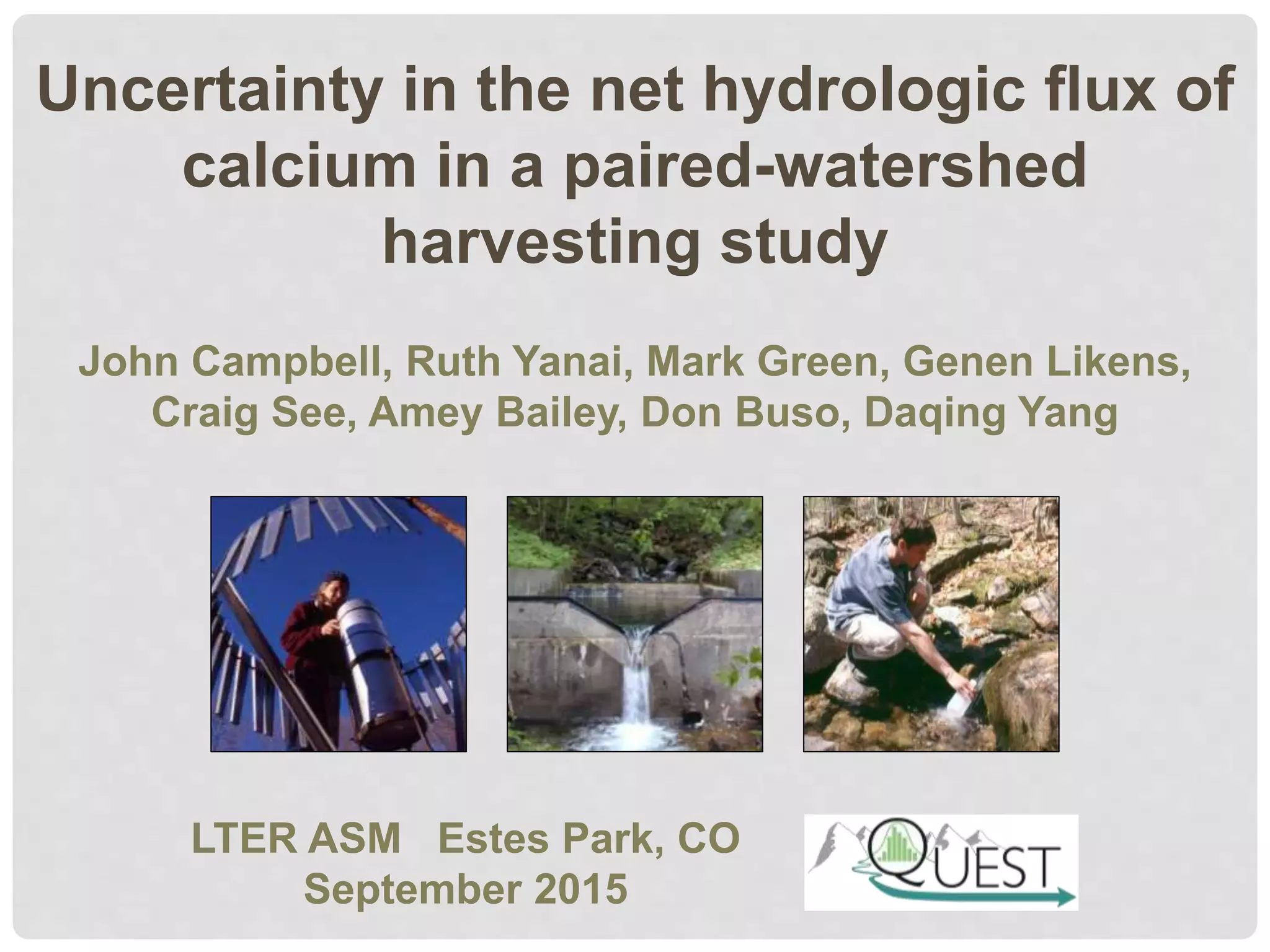
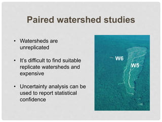
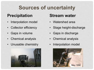
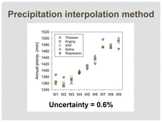
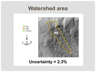
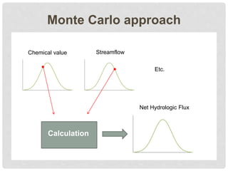
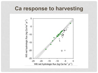
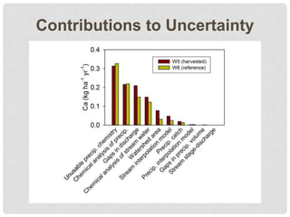
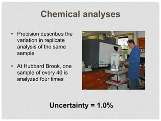
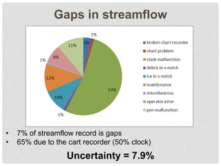
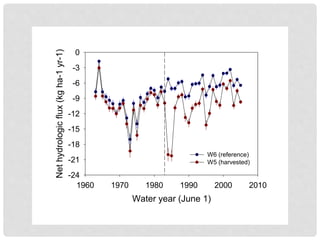
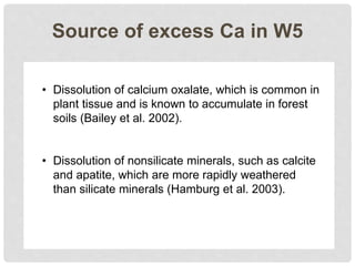
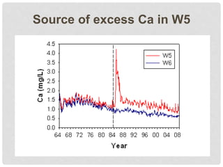
From all comments received by the LTER Network Office, this year's meeting in Estes Park was a complete success! The 2015 LTER All Scientists Meeting was held from August 30 through the evening of September 2. The Conference was organized around the theme: " From Long-Term Data to Understanding: Toward a Predictive Ecology". Almost 600 people attended the meeting. There were over 300 poster presentations and more than 75 formal and ad-hoc working group meetings. Drs. James Olds, Diana Wall, Knute Nadelhoffer, Ned Gardener and Christine O'Connell provided excellent plenary presentations to highlight the meeting. Chloe Wardropper (NTL) won 1st place in the student poster competition with Alexandra Conway (BNZ), Shinjini Goswami (HBR), Hafsah Nahrawi (GCE) and Bonnie McGill (KBS) winning runner-up awards.
❤Jammu Kashmir Call Girls 8617697112 Personal Whatsapp Number 💦✅.
Campbell 2015 lter asm v0.1 quest
1. Uncertainty in the net hydrologic flux of
calcium in a paired-watershed
harvesting study
LTER ASM Estes Park, CO
September 2015
John Campbell, Ruth Yanai, Mark Green, Genen Likens,
Craig See, Amey Bailey, Don Buso, Daqing Yang
2. Paired watershed studies
W6
W5
• Watersheds are
unreplicated
• It’s difficult to find suitable
replicate watersheds and
expensive
• Uncertainty analysis can be
used to report statistical
confidence
3. Ca response to harvesting
Harvest
Harvest
Data courtesy G.E. Likens
4. Sources of uncertainty
Precipitation
• Interpolation model
• Collector efficiency
• Gaps in volume
• Chemical analysis
• Unusable chemistry
Stream water
• Watershed area
• Stage height-discharge
• Gaps in discharge
• Chemical analysis
• Interpolation model
May 1956
11. Chemical analyses
Uncertainty = 1.0%
• Precision describes the
variation in replicate
analysis of the same
sample
• At Hubbard Brook, one
sample of every 40 is
analyzed four times
12. Acknowledgments
Calcium data were obtained through funding from the
A.W. Mellon Foundation and the NSF, including LTER
and LTREB.
Amey Bailey
Ian Halm
Nick Grant
Tammy Wooster
Branda Minicucci
13. Gaps in streamflow
• 7% of streamflow record is gaps
• 65% due to the cart recorder (50% clock)
Uncertainty = 7.9%
14. Easier said than done…
• Difficult to identify
sources of uncertainty
• Difficult to quantify
sources
• Multiple approaches to
uncertainty analysis
• No single answer
16. Source of excess Ca in W5
• Dissolution of calcium oxalate, which is common in
plant tissue and is known to accumulate in forest
soils (Bailey et al. 2002).
• Dissolution of nonsilicate minerals, such as calcite
and apatite, which are more rapidly weathered
than silicate minerals (Hamburg et al. 2003).
Alright, so we’ve been working on the issue of how to quantify uncertainty in watershed studies. And today I going to present results from a first pass at this where we quantified the uncertainty in the net hydrologic flux of calcium in a paired watershed study at Hubbard Brook. And this work was recently submitted to a special issue of Ecosphere on uncertainty analysis.
In paired watershed studies, like those that have occurred at Hubbard Brook, a manipulated watershed is compared to a nearby unmanipulated reference watershed. And these types of experiments have really been invaluable in understanding how ecosystems respond to disturbance. A common criticism of the experimental design is that the watersheds aren’t replicated . And the reason they’re not replicated is because it’s difficult to find suitable replicates and is expensive because of the scale of the experiments. So uncertainty analysis can help address this issue because it enables us to report statistical confidence even when replicates are not used.
The example we’ll use is the response of Calcium to the whole tree harvest in W5. This graph shows the net hydrologic flux so it’s the inputs in precipitation minus the outputs in streamwater. Watershed 5 which is indicated in red here was cut during the winter of 1983/84. And you can see that the net losses of Calcium are greater from the harvested watershed and that the increases appears to have persisted for many years after that. And in this example we want to know the differences between watersheds is greater than the uncertainty of the values. And so the goal is to produce measures of uncertainty to evaluate these differences in calcium between watersheds.
As a first step we try to identify the major potential sources of uncertainty in precipitation and streamwater. This is not an exhaustive list. There are many sources of uncertainty in watershed studies and what’s listed here is what we think are the most important sources that we were able to quantify. Some are missing, but I think we have most of the major sources represented.
I don’t have time to go into how we tried to quantify each of these sources of uncertainty so I’ll just highlight a couple. One is the method of interpolation for calculating the amount of precipitation falling on a watershed based on data from individual rain gages. We compared 5 different interpolation methods and found that the uncertianty for method selection is small, amounting 0.6% across watersheds.
Method is based on the mean deviation from the mean.
Calculate the deviation from the mean for each method, sum them, and divide by the mean
Could also calculate the standard deviation and divide by the mean. Both give you comparable results.
Another example is the uncertainty in the watershed area is relevant to the streamwater flux. The watershed was initially delineated with a ground survey, we can compare that with a watershed delineation using a DEM generated from LiDAR. We get slightly different estimates with each method and I think it’s fair to say that we don’t know which is better. And so the uncertainty in the watershed boundary is 2.3%. Of course the real watershed boundaries are belowground and maybe someday we’ll have a better way to measure the watershed area.
So those are just two of the examples of uncertainties involved in the calculation of the net hydrologic flux. To quantify the overall uncertainty in the net hydrologic flux we used a monte carlo approach whereby we randomly sampled from individual distributions of all these different variables. And we do that a 1000 times, and the result is a distribution of the net hydrologic flux.
So this monte carlo technique enables us to put error bars on our data. If you recall from the time series graph, there were differences in the net hydrologic flux of calcium before the treatment. So values from W6 were greater than the values for W5. So Another way of looking at this is by comparing the uncertainty in the post treatment values with the regression line for the pretreatment period. So the green circles are for the pretreatment period and the 95% confidence intervals of the regression line are show by the lighter lines. And the crosses are the data from after the harvest. The points farthest away from the line are the years after the cut and some of the points closest to the line are the most recent years of data. And you can see now that we have uncertainty represented, that the post harvest values are still greater than the uncertainty in the estimates, although a couple of values are very close to intersecting the pre-treatment regression line.
One of the neat things about this Monte Carlo approach is that you can evaluate the importance of individual sources of uncertainty. We do this by running the Monte Carlo with all the uncertainty calculations turned off except for the one we’re interested in. If we compare the contributions of each source of uncertainty evaluated we can see the greatest source of uncertainty is unusable precipitation chemistry, or chemistry samples that have been contaminated. So if we want to improve estimates we could collect more precipitation chemistry samples. Some of these sources are really quite small and could probably be ignored at least at this site. So I think I’ll end there and I’d be happy to take any questions you have. Thanks.
We also have uncertainty in the chemical analysis for both precipitation and stream water. Precision describes the variation in repeated analysis of the same sample. So you can run a sample over and over again and get an estimate of uncertainty. At Hubbard Brook one out of every 40 samples is analyzed 4 times. We used that to calculate the analytical uncertainty for calcium, which is about 1% (0.03 mg/L) and that’s fairly low compared to some of the other solutes we measure, such as nitrate and ammonium.
uncertainty in chemical analysis is commonly reported and generally small
Precision describes the variation in replicate analysis of the same sample
0.033 mg/L or one percent
1999-2011
We report precision as the average standard deviation of replicate samples in units of concentration and as the coefficient of variation (CV), or standard deviation divided by the mean
So this monte carlo technique enables us to put error bars on our data. And here the error bars indicate the interquartile range.
The last example I’ll show is gaps in the streamflow record. Craig See has been working on uncertainty due to gaps in the record. Amey Bailey provided information on historic gaps in the record. And she found that gaps make up about 9% of the streamflow record. It ‘s interesting that about 65% of the gaps are due to the cart recorder in general and about half of the gaps in the streamflow record are specifically due to failures with the clock on the chart recorder. So hopefully we’ll be able to reduce the number of gaps by replacing these chart recorders with the new shaft encoders that have been installed.
To get at the uncertainty, Craig wrote a program that randomly generates fake gaps, fills the gap based on regression from the reference watershed, then gives the difference between the prediction and the actual observation. This is done thousands of times. Based on this method we estimated that the uncertainty due to gaps in the streamflow record is
Amey analyzed the record from 1996-2009 – 14 years of data.
Update this pie chart with the half hourly data that craig see sent. It’s in a folder called gaps in a file named A-35 notes.
You have to say something about the flume also.
Of course this is easier said than done. The cartoon here says that I thought I was interested in uncertainty, but now I’m not so sure, which kind of summarizes how I feel. And the reason why these uncertainty analyses are complex is that it’s difficult to identify the various sources of uncertainty, once you’ve ideintified the sources it’s even more difficult to quantify the sources. There are many different approaches to uncertainty analysis, and there’s no single answer, you can always find ways to improve the results.