Alignment in Excel

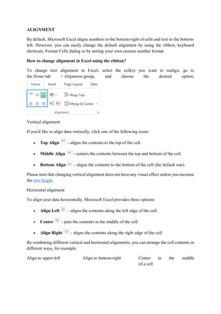
1. ALIGNMENT
By default, Microsoft Excel aligns numbers to the bottom-right of cells and text to the bottom-
left. However, you can easily change the default alignment by using the ribbon, keyboard
shortcuts, Format Cells dialog or by setting your own custom number format.
How to change alignment in Excel using the ribbon?
To change text alignment in Excel, select the cell(s) you want to realign, go to
the Home tab > Alignment group, and choose the desired option:
Vertical alignment
If you'd like to align data vertically, click one of the following icons:
 Top Align - aligns the contents to the top of the cell.
 Middle Align - centers the contents between the top and bottom of the cell.
 Bottom Align - aligns the contents to the bottom of the cell (the default one).
Please note that changing vertical alignment does not have any visual effect unless you increase
the row height.
Horizontal alignment
To align your data horizontally, Microsoft Excel provides these options:
 Align Left - aligns the contents along the left edge of the cell.
 Center - puts the contents in the middle of the cell.
 Align Right - aligns the contents along the right edge of the cell.
By combining different vertical and horizontal alignments, you can arrange the cell contents in
different ways, for example:
Align to upper-left Align to bottom-right Center in the middle
of a cell

2. Change text orientation (rotate text)
Click the Orientation button on the Home tab, in the Alignment group, to rotate text up or
down and write vertically or sideways. These options come in especially handy for labeling
narrow columns:
Indent text in a cell
In Microsoft Excel, the Tab key does not indent text in a cell like it does, say, in Microsoft
Word; it just moves the pointer to the next cell. To change the indentation of the cell contents,
use the Indent icons that reside right underneath the Orientation button.
To move text further to the right, click the Increase Indent icon. If you have gone too far right,
click the Decrease Indent icon to move the text back to the left.
Shortcut keys for alignment in Excel
To change alignment in Excel without lifting your fingers off the keyboard, you can use the
following handy shortcuts:
 Top alignment - Alt + H then A + T
 Middle alignment - Alt + H then A + M
 Bottom alignment - Alt + H then A + B

3.  Left alignment - Alt + H then A + L
 Center alignment - Alt + H then A + C
 Right alignment - Alt + H then A + R
At first sight, it looks like a lot of keys to remember, but upon a closer look the logic becomes
obvious. The first key combination (Alt + H) activates the Home tab. In the second key
combination, the first letter is always "A" that stands for "alignment", and the other letter
denotes the direction, e.g. A + T - "align top", A + L - "align left", A + C - "center alignment",
and so on.
To simplify things further, Microsoft Excel will display all alignment shortcuts for you as soon
as you press the Alt + H key combination:
How to align text in Excel using the Format Cells dialog
Another way to re-align cells in Excel is using the Alignment tab of the Format Cells dialog
box. To get to this dialog, select the cells you want to align, and then either:
 Press Ctrl + 1 and switch to the Alignment tab, or
 Click the Dialog Box Launcher arrow at the bottom right corner of the Alignment

4. In addition to the most used alignment options available on the ribbon, the Format Cells dialog
box provides a number of less used (but not less useful) features:
Now, let's take a closer look at the most important ones.
Text alignment options
Apart from aligning text horizontally and vertically in cells, these options allow you to justify
and distribute the cell contents as well as fill an entire cell with the current data.
How to fill cell with the current contents
Use the Fill option to repeat the current cell content for the width of the cell. For example, you
can quickly create a border element by typing a period in one cell,

5. choosing Fill under Horizontal alignment, and then copying the cell across several adjacent
columns:
How to justify text in Excel
To justify text horizontally, go to the Alignment tab of the Format Cells dialog box, and select
the Justify option from the Horizontal drop-down list. This will wrap text and adjust spacing
in each line (except for the last line) so that the first word aligns with the left edge and last
word with the right edge of the cell:
The Justify option under Vertical alignment also wraps text, but adjusts spaces between lines
so the text fills the entire row height:
How to distribute text in Excel
Like Justify, the Distributed option wraps text and "distributes" the cell contents evenly across
the width or height of the cell, depending on whether you enabled Distributed horizontal or
Distributed vertical alignment, respectively.
Unlike Justify, Distributed works for all lines, including the last line of the wrapped text. Even
if a cell contains short text, it will be spaced-out to fit the column width (if distributed
horizontally) or the row height (if distributed vertically). When a cell contains just one item
(text or number without in-between spaces), it will be centered in the cell.
This is what the text in a distributed cell looks like:
Distributed horizontally Distributed vertically Distributed horizontally
& vertically

6. When changing the Horizontal alignment to Distributed, you can set the Indent value, telling
Excel how many indent spaces you want to have after the left border and before the right border.
If you don't want any indent spaces, you can check the Justify Distributed box at the bottom
of the Text alignment section, which ensures that there are no spaces between the text and cell
borders (the same as keeping the Indent value to 0). If Indent is set to some value other than
zero, the Justify Distributed option is disabled (grayed out).
The following screenshots demonstrate the difference between distributed and justified text in
Excel:
Justified horizontally Distributed horizontally Justify distributed
Tips and notes:
 Usually, justified and/or distributed text looks better in wider columns.
 Both Justify and Distributed alignments enable wrapping text In the Format
Cells dialog, the Wrap text box will be left unchecked, but the Wrap Text button on the
ribbon will be toggled on.
 As is the case with text wrapping, sometimes you may need to double click the
boundary of the row heading to force the row to resize properly.
Center across selection
Exactly as its name suggests, this option centers the contents of the left-most cell across the
selected cells. Visually, the result is indistinguishable from merging cells, except that the cells
are not really merged. This may help you present the information in a better way and avoid
undesirable side-effects of merged cells.

7. Text control options
These options control how your Excel data is presented in a cell.
Wrap text - if the text in a cell is larger than the column width, enable this feature to display
the contents in several lines.
Shrink to fit - reduces the font size so that the text fits into a cell without wrapping. The more
text there is in a cell, the smaller it will appear.
Merge cells - combines selected cells into one cell.
The following screenshots show all text control options in action.
Wrap text Shrink to fit Merge cells
Changing text orientation
The text orientation options available on the ribbon only allow to make text vertical, rotate text
up and down to 90 degrees and turn text sideways to 45 degrees.
The Orientation option in the Format Cells dialog box enables you to rotate text at any angle,
clockwise or counterclockwise. Simply type the desired number from 90 to -90 in
the Degrees box or drag the orientation pointer.
Changing text direction
The bottom-most section of the Alignment tab, named Right-to-left, controls the text reading
order. The default setting is Context, but you can change it to Right-to-Left or Left-to-Right. In
this context, "right-to-left" refers to any language that is written from right to left, for example
Arabic.
Menus, Tabs, Toolbars and their Icons
The Home tab is where you manage the formatting and appearance of your sheet, along with
some simple formulas you’ll always need.

8. A. Copy and Paste Tools: Use these tools to quickly duplicate data and format styles in the
spreadsheet. The Copy tool can either copy a selected cell or group of cells, or copy an area of
the spreadsheet that you’ll use as a picture in another document. The Cut tool moves the
selection of cells to a new destination rather than duplicating it.
The Paste tool can paste anything in your clipboard into the selected cell, and typically retains
everything including the value, formula, and format. However, Excel has a wealth of pasting
options: you can access these by clicking the down arrow next to the Paste icon. You can paste
what you’ve copied as a picture. You can also paste what you’ve copied as values only, so that
instead of duplicating the formula of a copied cell, you duplicate the final value shown in the
cell.
The Format paintbrush copies everything related to the formatting of a selected cell. When you
select a cell and click Format, you can then highlight a whole range of cells, and each one will
take on the formatting of the original cell, without changing their values.
B. Visual Formatting Tools: Many of these tools are similar to those found in Microsoft
Word. You can use the formatting tools to change the font, size, and color of typed words, and
make them bold, italicized, or underlined. It also has a couple spreadsheet-specific formatting
options. You can choose which sides of the cell get additional borders, and their style and
thickness. You can also change the highlight color of the entire cell. This is useful for creating
visually-appealing borders or differentiating rows or columns on large sheets, or for
highlighting a particular cell that you want to accentuate.
C. Position Formatting Tools: Align cell data to the top, bottom, or middle of the cell. There
is also an option for angling the values displayed, which can make it easier to read. The bottom
row has familiar options for left, center, and right alignment. There are also indent right and
left buttons.
D. Multi-cell Formatting Features: This section contains two very important features that
solve common problems for new Excel users. The first is Wrap Text. Normally, when you enter
text into a cell that extends beyond the size of the cell, it spills into the next cell. For example,
if you type “Budgeted Items” into A1, some of the word “Items” spills into B1. Then, if you
type into B1, you cover up any characters from A1 that extended into B1. The extra text from
cell A1 still exists, but now it is hidden. If you don’t want to widen the cells, click the Wrap
Text icon on A1 - this will split “Budgeted Items” into two stacked lines instead of one within
A1. This makes the entire row taller to accommodate the content. Now, typing into B1 won’t
cover up existing text.

9. The other tool in this section is Merge and Center. There are instances when you may want to
combine several cells and have them act as one long cell. For example, you might want a header
for an entire table to be clear and easy to read. Select all the cells you want combined,
click Merge, and then type your header and format it. Though the default setting for headers is
centered text, simply click the drop-down arrow to select different merging and unmerging
options.
E. Numbers-based Format Settings: A drop-down menu has options for number formatting.
For example, currency places everything you select into “$0.00” format, and percent turns .5
or ½ into “50%”, date options. These are the basic format options, but you can select More
Number Formats from the drop-down menu to get more specialty use cases (different
countries’ currencies, or adding the “(xxx)xxx-xxxx” formatting to phone number sequences).
Often, you may use these tools on entire columns to make all data in one category behave the
same way.
F. Table or Sheet Formatting: Format as Table and Cell Styles allow you to use presets or
customize tables (for example, with alternating row colors and highlighted header bars). Select
your data range and choose a style to standardize formatting.
Conditional formatting is a bit more complex. Use the drop-down menu to select from a range
of options, like inserting helpful visual icons to represent status or completion, or changing the
color of different rows. Most important are the conditional rules, which are created with a
simple logic. For example, let’s say you have a column with data in A1 through A3, and A4
holds the sum of these three cells. You could place formatting on A4 with a rule that says “if
A4 > 0, then highlight A4 green.” Then, you could add another rule that says “if A4 < 0, then
highlight A4 red.” Now you have a quick visual reference where green = a positive number
and red = a negative number, which will change based on what you enter into A1, A2, and A3.
G. Row and Column Formatting Tools: The Insert drop-down menu puts cells, rows, or
columns before or after a selected area on the sheet, and Delete removes them.
The Format drop-down lets you change the height of rows and the width of columns. It also
has options for hiding and unhiding certain sections.
H. Miscellaneous Tools: Starting at the top left, there’s AutoSum, which allows you to select
a swath of cells and place the sum in the cell located right below or directly to the right of the
last selected data point. You can use the drop-down to change the function to calculate the
average, display the maximum, minimum, or the count of numbers selected.
Use Fill to take a cell’s contents and extend them in any direction for as many cells as you
want. If the cell contains a value, Fill will simply copy the value over and over again. If it
contains a formula, it will recalculate its relative position for each new cell. If the first cell
equals A1+B1, then the next would equal A2+B2, and so on.
The Clear button lets you either clear the value, or just clear cell formatting.
Sort & Filter tools let you choose what to display, and in what order. At the base level, this
tool sorts cells containing text from A to Z, and cells containing numbers from lowest to

10. highest. It can also sort by color or icon. Sorting and filtering helps surface only the data you
need.
Use the Insert tab to add extra elements to your Excel workbook that go beyond text and colors.
A. These tools control PivotTables, an important Excel function. Think of PivotTables as
“reports,” a quick way to view all your data, analyze trends, and draw conclusions. By selecting
at least two rows of data and clicking on PivotTable, you can quickly generate a visually-
appealing table. Going through this process launches the PivotTable Builder, which helps you
select columns to include, sort them, and drag-and-drop them to quickly construct your table.
They can include collapsible rows to make reports interactive and uncluttered. There is also a
button for Recommended PivotTables, which can help when you don’t know where to start.
Table builds a simple table that includes any number of columns you select. Rather than placing
the table elsewhere on the worksheet, it turns the data into a table on the spot, and applies
customizable color formatting.
B. This section lets you insert visual elements, like picture files, pre-built shapes, and SmartArt.
You can add shapes and resize, recolor, and reposition them to create intuitive data sets and
reports. SmartArt objects are prebuilt diagrams that you can insert text and information into.
They’re great for representing what the data says in another place on your workbook.
C. These tools are for inserting elements from other Microsoft products, like Bing Maps, pre-
built information cards about People (from Microsoft accounts only), and add-ins from their
store.
D. Use these tools to create charts and graphs. Most of them work only if you select one or
more data sets (numbers only, with words for headers or categories). Charts and graphs
function like you’d expect - just select the data you want to visualize, then select your desired
type of visual (bar charts, scatter plots, pie charts, or line graphs). Creating one will bring up
formatting options where you can change the color, labels, and more.
E. Sparklines are more simplistic graphs that can fit in as little as one cell. You can place them
next to data for a small, quick visual representation.
F. Slicers are big lists of buttons that make your data more interactive. You can select
a PivotTable you’ve created, and then create a slicer from it - this allows a viewer to click on
buttons that correlate to the data they want to filter.
G. This hyperlink tool allows you to make a cell or table into a clickable link. Once a viewer
clicks on the affected cell(s), they’ll be taken to whatever website or intranet site you select.

11. H. Recent versions of Excel allow for better collaboration - insert comments on any cell or
range of cells to add more context. You can open or close the comments so the worksheet
doesn’t get too cluttered.
I. A Text Box is useful when you’re creating a report and don’t want typed words to behave
like cells. It makes it easy to move your text around, rather than cutting and pasting cells (which
could potentially mess up the formatting of real data). The next area is for Headers & Footers,
which will take you to the page layout view - here you can add headers and footers for the
entire page. WordArt, on the other hand, lets you embellish text. Insert Object lets you place
entire files (Word documents, PDFs, etc.) into the worksheet.
J. This section lets you insert Equations and Symbols. Use equations to write a math equation
with fractions, variables, and more that you can place in your sheet like a Text Box. For
instance, this can be helpful for explaining how a portion of a table was calculated in a
report. Symbols, on the other hand, can be inserted directly into cells, and include all non-
standard characters from most languages, as well as emojis.
The Page Layout tab has everything you need to change the structural parts of your worksheet,
especially for purposes of printing or presenting.
A. Use these buttons to quickly adjust the visual style of your entire sheet. You can regulate
the fonts and colors, and use the Themes section to quickly apply it to every table, PivotTable,
and SmartArt element for a clean, well-designed sheet.
B. These are print options. You can change the margin for printing, whether you want a vertical
or horizontal print alignment, which cells in your sheet you want to print, where you’d like
page breaks, and whether it has a background (to place your company name, for example). You
can also start giving each page a heading using the Print Titles button, and the order to print
each section.
C. This lets you choose how many pages across and how many pages down you’d like to print.
D. This section lets you toggle whether the automatic grids appear for working on the sheet
and for printing it, along with the row and column headings (A, B, C, 1, 2, 3, etc).
The Formulas tab stores nearly everything related to Excel’s reputation as “complex.”
Because this article is intended for beginners, we won’t cover every function is this section
thoroughly.

12. A. The Insert Function button is useful for those who don’t know all the shorthand. This brings
up a side Formula Builder section that describes each function, and you can select the one you
want to use.
B. These buttons divide all the functions by category.
 AutoSum works the same as it does in the Home tab.
 Recently Used is helpful for bringing up frequently used formulas to save time looking
through menus.
 Financial includes everything related to currency, values, depreciation, yield, rate, and
more.
 Logical includes conditional functions, like “IF X THEN Y.”
 Text functions help clean, regulate, and analyze plain text cells, such as displaying the
character count of a cell (helpful for Twitter posts), combining two different rows
via Concatenate, or pulling out numerical values from text entries that aren’t formatted
correctly.
 Date & Time functions help make meaning out of time-formatted cells, and include
entries like “TODAY,” which enters the current date.
 Lookup & Reference functions help pull information from different parts of your
workbook to save you the trouble of looking for them.
 Math & Trig functions are just what they sound like, involving every sort of math
discipline you can imagine.
 More Functions includes Statistical and Engineering data.
C. This section contains tagging options. If there’s a range of cells or a table you frequently
need to refer to in formulas, you can define its name and tag it here. For example, say you had
a column that contained the entire list of products you sell. You could highlight the names in
that list and Define Name as “ProductList.” Every time you want to refer to that column in a
formula, you can simply type “ProductList” (rather than finding that collection of data again
or memorizing their cell positions).
D. This contains error checking tools. With Trace Precedents and Trace Dependents, you can
see which cells contain formulas that refer to a given cell and vice versa. Show
Formulas reveals the formulas inside all cells, rather than their display values. Error
Checking automatically finds broken links and other issues with your spreadsheet.

13. E. Should you have a large sheet with a massive series of interconnected formulas, tables and
cells, you can use this section to trigger calculations, and also to choose which types of data
don’t run. A good example is a mortgage or asset depreciation sheet.
The Data tab is for performing more complex data analysis than most beginners will
need.
A. These are database import tools, allowing you to import data from any web, file, or server-
based database.
B. This section helps you fix database connections, refresh data, and adjust properties.
C. These are Sort and Filter options similar to those for data you have within your sheet,
applied to data feeds. They’re especially crucial here as a database is sure to have more data
than you can or care to use.
D. These are data manipulation tools. You can take a single long string, like those separated by
commas or spaces, and divide them into columns with Text to Columns. You can seek and
remove duplicates, consolidate cells, and validate whether data meets certain criteria to assess
its accuracy. What-if Analysis helps you fill in gaps with incomplete data using existing data
and trends to determine likely outcomes for new scenarios.
E. These tools help you manage how much data you have to deal with at once and group them
by whatever criteria you deem necessary. It’s similar to sorting, but you can choose any range
of columns or rows and make them collapsible, each with their own label. Use Subtotal to
create automatic calculations along a data set by different categories, which is helpful for
financial sheets.
The Review tab is part of the Ribbon that helps with sharing and accuracy checks.
A. These are simple text-based checks (like in Word) that allow you to locate cells with spelling
errors, or find more appropriate words via the Thesaurus.

14. B. Check Accessibility pulls up errors that can make it difficult to access the data in other
programs, or just for reading purposes. It might find that your sheet is missing alt text, or that
you’re using defaults for sheet names that can make navigation less intuitive.
C. The commenting tools allow collaborators to “talk” to each other within the sheet.
D. Protecting and sharing tools allow you to invite collaborators and restrict access to certain
parts of the sheet. You can manually assign different levels of access - for example, you might
allow a contractor to edit just the cells related to the hours they worked, but not the cells that
calculate their pay. As with Word, sharing a sheet with Tracked Changes means you can see
everything that’s been done to the sheet.
E. When you’ve shared a workbook, you can restrict permissions later on using this button and
selecting individual contributors.
Use the tools in the View tab to change settings related to what you can see or do.
A. This is your basic view where you can see your default sheet view, how it’ll look when
printing, and in custom ways you set yourself.
B. Use these buttons to choose whether you want to see the grids, headings, formula bar, and
ruler.
C. This is another way to control zooming in and out of cells.
D. Freeze Pane controls are an important part of making a usable spreadsheet. Using these
tools, you can freeze a number of rows and/or columns while you scroll around. For example,
if the first row had all your column headings and remained frozen, you’ll always know which
column you are looking at as you scroll down.
E. Macros are a way of automating processes in Excel. It is far beyond Excel 101, however.