SlideShare a Scribd company logo
1 of 144
Download to read offline
Feedback Control Methods for a Single Machine Infinite
Bus System
Pratik Vernekar, Zhongkui Wang, Andrea Serrani, and Kevin Passino
Department of Electrical and Computer Engineering, The Ohio State University
2015 Neil Avenue, Columbus, OH 43210
Email: pratik.vernekar@gmail.com,
wang.1231@osu.edu,
serrani.1@osu.edu,
passino.1@osu.edu
Abstract
In this manuscript, we present a high-fidelity physics-based truth model of a Single Machine Infinite
Bus (SMIB) system. We also present reduced-order control-oriented nonlinear and linear models of a
synchronous generator-turbine system connected to a power grid. The reduced-order control-oriented
models are next used to design various control strategies such as: proportional-integral-derivative (PID),
linear-quadratic regulator (LQR), pole placement-based state feedback, observer-based output feedback,
loop transfer recovery (LTR)-based linear-quadratic-Gaussian (LQG), and nonlinear feedback-linearizing
control for the SMIB system. The controllers developed are then validated on the high-fidelity physics-
based truth model of the SMIB system. Finally, a comparison is made of the performance of the controllers
at different operating points of the SMIB system. The material presented in this manuscript is part of
a course on “Control and Optimization for the Smart Grid” that was developed in the Electrical and
Computer Engineering Department at the Ohio State University in 2011-2012. This project was funded
by the U.S. Department of Energy.
1
Contents
1 A Single Generation Unit 4
2 Truth Model of the Synchronous Generator 5
2.1 Electrical Dynamics . . . . . . . . . . . . . . . . . . . . . . . . . . . . . . . . . . . . . . . . . 6
2.1.1 Voltage Equation in the Static Frame . . . . . . . . . . . . . . . . . . . . . . . . . . . 6
2.1.2 Voltage Equation in the Synchronously Rotating Frame . . . . . . . . . . . . . . . . . 8
2.1.3 Voltage Equation of the Synchronous Generator in Per Unit System . . . . . . . . . . 10
2.2 A Synchronous Generator Connected to an Infinite Bus . . . . . . . . . . . . . . . . . . . . . 10
2.3 Mechanical Dynamics: Swing Equation . . . . . . . . . . . . . . . . . . . . . . . . . . . . . . . 11
2.4 Truth Model of the Synchronous Generator . . . . . . . . . . . . . . . . . . . . . . . . . . . . 14
2.5 Model of the Turbine-Governor System . . . . . . . . . . . . . . . . . . . . . . . . . . . . . . . 17
2.6 Truth model of the combined Synchronous Generator and Turbine-Governor System con-
nected to an infinite bus . . . . . . . . . . . . . . . . . . . . . . . . . . . . . . . . . . . . . . . 18
2.7 Derivation of the Output Generator Terminal Voltage for the Truth Model . . . . . . . . . . . 18
3 The Reduced Order Simplified Model 20
3.1 Reduced order model of the combined Synchronous Generator and Turbine-Governor system
connected to an infinite bus . . . . . . . . . . . . . . . . . . . . . . . . . . . . . . . . . . . . . 20
3.2 Derivation of the Output Generator Terminal Voltage for the Reduced Order Model . . . . . 23
3.3 Linearization of the Reduced Order Model by Taylor series approximation . . . . . . . . . . . 25
3.4 Example . . . . . . . . . . . . . . . . . . . . . . . . . . . . . . . . . . . . . . . . . . . . . . . . 30
4 Open Loop Input-Output Behavior of the Synchronous Generator and Turbine-Governor
System 34
5 The Decoupled Reduced Order Model 41
5.1 LFC Dynamics . . . . . . . . . . . . . . . . . . . . . . . . . . . . . . . . . . . . . . . . . . . . 42
5.1.1 PID controller design for the LFC loop . . . . . . . . . . . . . . . . . . . . . . . . . . . 46
5.2 AVR Dynamics . . . . . . . . . . . . . . . . . . . . . . . . . . . . . . . . . . . . . . . . . . . . 48
5.2.1 PID controller design for the AVR loop . . . . . . . . . . . . . . . . . . . . . . . . . . 50
5.3 LFC and AVR including coupling . . . . . . . . . . . . . . . . . . . . . . . . . . . . . . . . . . 52
6 PID Controller Design 53
6.1 PID Controller Design based on linear model . . . . . . . . . . . . . . . . . . . . . . . . . . . 53
6.2 Simulation results for the PID Controllers applied to the Reduced Order Nonlinear Model . . 56
6.3 Simulation results for the PID Controllers applied to the Truth Model . . . . . . . . . . . . . 59
7 Linear State-Space Controller Design 62
7.1 State Feedback Controller design using LQR methodology . . . . . . . . . . . . . . . . . . . . 62
7.1.1 LQR Design based on linear model . . . . . . . . . . . . . . . . . . . . . . . . . . . . . 62
7.1.2 Simulation results for the Full-State Feedback LQR applied to the Reduced Order
Nonlinear Model . . . . . . . . . . . . . . . . . . . . . . . . . . . . . . . . . . . . . . . 65
7.1.3 Simulation results for the Full-State Feedback LQR applied to the Truth Model . . . . 69
7.2 State Feedback Controller design using Pole Placement Technique . . . . . . . . . . . . . . . 72
7.2.1 Pole Placement Design based on linear model . . . . . . . . . . . . . . . . . . . . . . . 72
7.2.2 Simulation Results for the Full-State Feedback Pole Placement controller applied to
the Reduced Order Nonlinear Model . . . . . . . . . . . . . . . . . . . . . . . . . . . . 75
7.2.3 Simulation Results for the Full-State Feedback Pole Placement controller applied to
the Truth Model . . . . . . . . . . . . . . . . . . . . . . . . . . . . . . . . . . . . . . . 78
7.3 Output Feedback Controller Design . . . . . . . . . . . . . . . . . . . . . . . . . . . . . . . . . 81
2
7.3.1 Observer-based LQR Design based on linear model . . . . . . . . . . . . . . . . . . . . 81
7.3.2 Observer-Based Pole Placement Controller Design based on linear model . . . . . . . . 88
7.3.3 Simulation Results for the Observer-based LQR applied to the Reduced Order Non-
linear Model . . . . . . . . . . . . . . . . . . . . . . . . . . . . . . . . . . . . . . . . . 91
7.3.4 LTR-based LQG Controller applied to the Reduced Order Nonlinear Model . . . . . . 93
7.3.5 LTR-based LQG Controller applied to the Truth Model . . . . . . . . . . . . . . . . . 97
8 Nonlinear Feedback Linearizing Controller Design 100
8.1 Nonlinear Feedback Linearizing Controller Design for the Reduced Order Model . . . . . . . . 102
8.2 Simulation Results for the Nonlinear Feedback Linearizing Controller applied to the Truth
Model . . . . . . . . . . . . . . . . . . . . . . . . . . . . . . . . . . . . . . . . . . . . . . . . . 109
9 Simulation results for the Controllers at different Operating Points 114
9.1 Simulation results for the Controllers at Operating Point II . . . . . . . . . . . . . . . . . . . 115
9.2 Simulation results for the Controllers at Operating Point III . . . . . . . . . . . . . . . . . . . 119
10 Appendix 124
10.1 Derivation of Park’s Transformation . . . . . . . . . . . . . . . . . . . . . . . . . . . . . . . . 124
10.1.1 Stator and Rotor Inductances . . . . . . . . . . . . . . . . . . . . . . . . . . . . . . . . 124
10.1.2 Park’s Transformation . . . . . . . . . . . . . . . . . . . . . . . . . . . . . . . . . . . . 126
10.1.3 Voltage Equation in the Rotating Frame . . . . . . . . . . . . . . . . . . . . . . . . . . 127
10.2 Per Unit Conversion . . . . . . . . . . . . . . . . . . . . . . . . . . . . . . . . . . . . . . . . . 130
10.2.1 Choosing a base for stator quantities . . . . . . . . . . . . . . . . . . . . . . . . . . . . 131
10.2.2 Choosing a base for rotor quantities . . . . . . . . . . . . . . . . . . . . . . . . . . . . 131
10.2.3 The correspondence of per unit stator EMF to rotor quantities . . . . . . . . . . . . . 133
10.3 Sub-transient and Transient Inductances and Time Constants . . . . . . . . . . . . . . . . . . 133
10.3.1 Sub-transient and Transient Inductances . . . . . . . . . . . . . . . . . . . . . . . . . . 133
10.3.2 Time constants . . . . . . . . . . . . . . . . . . . . . . . . . . . . . . . . . . . . . . . . 135
10.4 Simplified Model of the Synchronous Generator . . . . . . . . . . . . . . . . . . . . . . . . . . 136
10.4.1 The two-axis model . . . . . . . . . . . . . . . . . . . . . . . . . . . . . . . . . . . . . 137
10.4.2 The one-axis or the third-order simplified model . . . . . . . . . . . . . . . . . . . . . 143
3
1 A Single Generation Unit
Fossil fuels such as coal, oil, and natural gas have been the main resources of electrical energy for many
years. However in recent years, there has been a gradual increase in the use of renewable energy resources
for electricity generation, such as hydro, biogas, solar, wind, and geothermal energy. Electricity generation
is basically the process of generating electric energy from other forms of energy. An electromechanical device
called synchronous generator driven by a prime mover, usually a turbine or a diesel engine, converts the
mechanical energy into alternating current (AC) electrical energy.
Synchronous
generator
Measuring
element
To grid through breakers and transformers
Governor
P
f
Pref
ω
Turbine
Working
fluidin
Valves
Working
fluidout
Shaft
Exciter
Automatic
voltage
regulator
Vt
It
Vref
Figure 1.1: Structure of a generation unit.
The system shown in Figure 1.1 is a general structure of a single generation unit [7]. The turbine extracts the
energy from the working fluid flowing into the turbine through valves. Typical working fluids are gas, steam,
and water. The shaft is the rotary part of the turbine on which the synchronous generator is mounted. The
opening and closing of the turbine valves or the frequency at which the turbine valves operate is regulated
to a reference frequency of fref, by a turbine governor. The frequency of the grid f which is measured by the
measuring element is directly related to the output power P. Thus, the output of the synchronous generator
P and the angular frequency of the shaft ω are measured and fed back to the governor by the measuring
element. Meanwhile, the measuring element also provides information about the output terminal voltage Vt
and output current It of the synchronous generator to the automatic voltage regulator (AVR), which is able
to control the terminal voltage of the synchronous generator to a reference voltage Vref through the exciter.
The excitation current generated by the exciter produces the magnetic field inside the generator.
Thus, from the above figure we can see that in an interconnected power system, where a synchronous
generator is connected to a grid, load frequency control (LFC) and automatic voltage regulator (AVR)
equipment is installed for each generator. Figure 1.1 shows two control loops, namely the load frequency
control (LFC) loop and the automatic voltage regulator (AVR) loop. The controllers are set for a particular
operating condition and accommodate small changes in load demand to maintain the frequency and voltage
magnitude within the specified limits. Small changes in real power are mainly dependent on changes in rotor
angle δ, and thus the frequency ω. The reactive power is mainly dependent on the voltage magnitude (i.e.,
on the generator excitation). The excitation system time constant which is an indication of how fast the
transients of the AVR loop decay exponential to zero, is much smaller than the prime mover time constant.
Thus the transients of the excitation system and thus the AVR loop decay much faster than the transients
of the LFC loop, hence it does not affect the LFC dynamics. Thus, the cross-coupling between the LFC loop
and the AVR loop is negligible. Hence, load frequency control and excitation voltage control are usually
analyzed independently [8].
4
The operation objectives of the LFC are to maintain reasonably uniform frequency, and to divide the
load between generators [8]. The change in frequency is sensed, which is a measure of the change in rotor
angle δ, i.e., the error ∆δ to be corrected. The error signal i.e., ∆f = fref − f is amplified, mixed, and
transformed into a real power command signal ∆PV = Pref − P, which is sent to the prime mover to call
for an increment in the torque. The prime mover, therefore, brings about a change in the generator output
which will change the value of ∆f within the specified tolerance.
The generator excitation system maintains the generator terminal voltage and controls the reactive power
flow. The generator excitation of older systems may be provided through slip rings and brushes by means
of DC generators mounted on the same shaft as the rotor of the synchronous machine. However, modern
excitation systems also known as brush-less excitation systems, usually use AC generators with rotating
rectifiers. The sources of reactive power are generators, capacitors, and reactors. The generator reactive
power is controlled by field excitation using the AVR. The role of an AVR is to hold the terminal voltage
magnitude of a synchronous generator at a specified level. An increase in the reactive power load of the
generator is accompanied by a drop in the terminal voltage magnitude. The voltage magnitude is sensed
through a potential transformer on one phase. This voltage is rectified and compared to a DC set point
signal. The amplified error signal controls the exciter field and increases the exciter terminal voltage. Thus,
the generator field current is increased, which results in an increase in the generated electromotiveforce
(emf). The reactive power generation is increased to a new equilibrium, raising the terminal voltage to the
desired value.
2 Truth Model of the Synchronous Generator
In the previous section we saw the basic working of a single generation unit and the respective roles of
the load frequency control and the automatic voltage regulator. In this section we will derive the truth
model of a synchronous generator. Before we proceed to the derivation of the truth model, we present some
preliminaries about the synchronous generator.
The two main parts of a synchronous generator can be described in either electrical or mechanical terms:
• Electrical:
– Armature: The power-producing component of an electrical machine. In a synchronous generator,
the armature windings generate the electric current. The armature can be on either the rotor or
the stator.
– Field: The magnetic field component of an electrical machine. The magnetic field of the syn-
chronous generator can be provided by either electromagnets or permanent magnets mounted on
either the rotor or the stator.
• Mechanical:
– Rotor: The rotating part of the synchronous generator.
– Stator: The stationary part of the synchronous generator.
Because power transferred into the field circuit is much smaller than in the armature circuit, AC generators
always have the field winding on the rotor and the stator has the armature winding. Thus, a classical
synchronous generator has two main magnetic parts: the stator and the rotor, as shown in Figure 2.1. The
windings are represented by one-turn coils, specifically, the small circles “⃝” in the figure. The black dots
and the crosses inside the small circles indicate the directions of the currents flowing in the windings, i.e.,
“×” means the current flowing in the direction from the outside of the paper vertically into the paper and
“•” means the current flowing from the inside of the paper to the outside.
5
×
×
×
×
×
×
a′
cb′
a
c′
b
D
F
D′
F′ QS
Q′
N
Rotor
Stator
Figure 2.1: Schematic structure of the synchronous generator.
The armature winding, which carries the load current It and supplies power to the grid, is placed in equidis-
tant slots on the inner surface of the stator and consists of three identical phase windings, namely, aa′,
bb′ and cc′. The rotor is mounted on the shaft through which the synchronous generator is driven by the
prime mover, for instance, a hydro turbine. The rotor consists of two poles, N pole and S pole, as seen in
Figure 2.1. The direct current (DC) excitation winding represented by FF′ is wrapped around the rotor.
From basic physics, we know that the DC flowing in the excitation winding generates a magnetic flux. Mag-
netic flux is a measure of the amount of magnetic field (also called magnetic flux density) passing through
a given surface (such as a conducting coil). The SI unit of magnetic flux is the weber (in derived units:
volt-seconds). The strength of the magnetic flux generated is proportional to the excitation current and its
direction is known by using the right-hand rule. As the rotor rotates, the magnetic flux generated by the
excitation winding wrapped on the rotor changes spatially. Thus, there are magnetic flux changes in the
armature windings as a result of which an emf is induced in each phase of the three-phase stator armature
winding. By connecting armature windings to the grid, a closed-loop circuit is formed which allows the AC
to flow from the synchronous generator to the grid. The AC armature currents produce their own armature
reaction magnetic flux which is of constant magnitude but rotates at the same speed as the rotor. The
excitation flux and the armature reaction flux then produce a resultant flux that is stationary with respect
to the rotor. Two other windings represented by DD′ and QQ′ are the two short-circuit damper (or, amor-
tisseur) windings which help to damp the mechanical oscillations of the rotor [2]. Hence, two dynamics will
characterize the generator, i.e., electrical dynamics and mechanical dynamics.
2.1 Electrical Dynamics
In this section we present the equations governing the electrical dynamics of a synchronous generator which
are described in [2]. We first present the voltage equations of a synchronous generator in the static frame,
and then use Park’s transformation to convert these to the rotating frame.
2.1.1 Voltage Equation in the Static Frame
In this subsection we present the voltage equations in the static frame. The static frame contains three
reference axes a, b, and c which correspond to the three armature windings on the stator. Before presenting
the details of the voltage equation of a synchronous generator, we start by considering the general case of a
set of coupled coils in which one or more of the coils is mounted on a shaft and can rotate. The situation is
shown schematically in Figure 2.2.
6
L1
R1i1
L2
R2
i2
L3
R3 i3
L4
R4 i4
Shaft
+ −v1
+
−
v2
+− v3+− v4
Figure 2.2: Coupled coils.
Assume that for any fixed shaft angle θ there is a linear relationship between the flux linkage λ and current
i. Flux linkage is defined as the total flux passing through a surface (i.e. normal to that surface) formed by
a closed conducting loop. Thus we get the relationship λ = L(θ)i, where, in the case of Figure 2.2, i and
λ are 4 × 1 vectors, and L is a 4 × 4 matrix. By applying Kirchhoff’s voltage law (KVL) to the circuit in
Figure 2.2, we have
v = Ri +
dλ
dt
(2.1)
where R is a 4 × 4 matrix. Equation (2.1) indicates that the terminal voltage of each coil equals the sum of
the voltage drop on the resistance and the derivative of the flux linkage.
7
×
×
×
×
×
×
θ
Reference
axis
Direct
axis
Quadrature
axis
a′
ia
c
icib b′
ia
a
c′ ib b
D
F
iD
iF
D′
F′
iQ
Q
Q′ × d
d′
id
×
q′
q
iq
Figure 2.3: Machine schematic.
By applying Equation (2.1) and using the circuits convention on the associated reference directions in
Figure 2.3, we get the relationship between voltages, currents, and flux linkages [2].








va′a
vb′b
vc′c
vFF′
vDD′
vQQ′








=








r
r 0
r
rF
0 rD
rQ
















ia
ib
ic
iF
iD
iQ








+
d
dt








λaa′
λbb′
λcc′
λFF′
λDD′
λQQ′








= Ri +
dλ
dt
(2.2)
We simplify the equation above by using a single-subscript notation, i.e., va vaa′ = −va′a, vb vbb′ = −vb′b,
vc vcc′ , vF vFF′ , vD vDD′ , and vQ vQQ′ . Here, we define v [va, vb, vc, −vF , −vD, −vQ]T to
be the voltage vector consisting of the three phase terminal voltages (va, vb, vc), and the voltage of the
field winding (vF ) and two damper windings (vD, vQ). The corresponding current vector is defined as
i [ia, ib, ic, iF , iD, iQ]T. Then Equation (2.2) can be written as follows:
v = −Ri −
dλ
dt
(2.3)
2.1.2 Voltage Equation in the Synchronously Rotating Frame
The electrical dynamics as given in Equation (2.2) are derived in the static abc frame. The flux linkage
in Equation (2.2) is dependent on the self and mutual inductances which are not constant, but are time
varying. In the voltage equation as given in Equation (2.3) the ˙λ term must be computed as ˙λ = L˙i + ˙Li.
Thus, to simplify the equations we make a coordinate transformation which transforms variables from the
abc static frame to a synchronously rotating frame (which is also called dq frame, see Figure 2.3). As a result
8
of this transformation we introduce two fictitious windings dd′ and qq′, as shown in Figure 2.3. Thus we get
vd = −rid − ωλq −
dλd
dt
vq = −riq + ωλd −
dλq
dt
vF = rF iF +
dλF
dt
vD = rDiD +
dλD
dt
vQ = rQiQ +
dλQ
dt
(2.4)
The details of the derivation of this transformation are given in the Appendix. The extra terms −ωλq and
ωλd are introduced by the transformation.
We can rearrange Equation (2.4) to put the quantities on the direct axis together and the quantities on
the quadrature axis together. Hence, Equation (2.4) is rewritten as follows:
vd = −rid − ωλq −
dλd
dt
vF = rF iF +
dλF
dt
vD = rDiD +
dλD
dt
vq = −riq + ωλd −
dλq
dt
vQ = rQiQ +
dλQ
dt
(2.5)
As the damper windings are short-circuited, the terminal voltages are both zero. As shown in Figure 2.3
the direct axis is perpendicular to the windings dd′, FF′, and DD′; the quadrature axis is perpendicular
to the windings qq′ and QQ′. Using the right hand thumb rule we can see that the flux linkage due to the
currents id, iF , and iD is along the direct axis and the flux linkage due to the currents iq and iQ is along
the quadrature axis. Thus, the flux linkage λd along the dd′ winding depends on the currents id, iF , and
iD and is given by λd = Ldid + kMF iF + kMDiD, where Ld is the self inductance of dd′ winding, MF is
the mutual inductance between dd′ and FF′ windings, and MD is the mutual inductance between dd′ and
DD′ windings, respectively. We can derive equations for λF and λD in a similar fashion. Also, the flux
linkage λq along the qq′ winding depends on the currents iq, and iQ and is given by λq = Lqiq + kMQiQ,
where Lq is the self inductance of the qq′ winding, and MQ is the mutual inductance between qq′ and QQ′
windings, respectively. We can derive λQ using the same approach. Also note that in Equation (2.6) and
Equation (2.7) which gives a relationship between the flux and the current in each winding, the mutual
inductance between the windings FF′ and DD′ is denoted by MR, and self-inductances of the windings are
denoted by Ld, LF , LD, Lq, and LQ, respectively. Thus, the connection between the flux and the current is
given by 

λd
λF
λD

 =


Ld kMF kMD
kMF LF MR
kMD MR LD




id
iF
iD

 (2.6)
and
λq
λQ
=
Lq kMQ
kMQ LQ
iq
iQ
(2.7)
where k = 3/2. If we substitute Equation (2.6) and Equation (2.7) into Equation (2.5) and put it in
9
matrix form, we obtain






vd
vF
0
vq
0






=






−r 0 0 −ωLq −ωkMQ
0 rF 0 0 0
0 0 rD 0 0
ωLd ωkMF ωkMD −r 0
0 0 0 0 rQ












id
iF
iD
iq
iQ






+






−Ld −kMF −kMD 0 0
kMF LF MR 0 0
kMD MR LD 0 0
0 0 0 −Lq −kMQ
0 0 0 kMQ LQ












˙id
˙iF
˙iD
˙iq
˙iQ






(2.8)
Moving the derivative of the current to the left-hand side, we obtain






Ld kMF kMD 0 0
−kMF −LF −MR 0 0
−kMD −MR −LD 0 0
0 0 0 Lq kMQ
0 0 0 −kMQ −LQ












˙id
˙iF
˙iD
˙iq
˙iQ






=






−r 0 0 −ωLq −ωkMQ
0 rF 0 0 0
0 0 rD 0 0
ωLd ωkMF ωkMD −r 0
0 0 0 0 rQ












id
iF
iD
iq
iQ






−






vd
vF
0
vq
0






(2.9)
2.1.3 Voltage Equation of the Synchronous Generator in Per Unit System
A normalization of variables called the per unit normalization is always desirable. The idea is to pick base
values for quantities such as voltages, currents, impedances, power, and so on, and to define the quantity in
per unit as
quantity in per unit =
actual quantity
base value of quantity
(2.10)
By carefully choosing the base quantities for both stator and rotor variables, the electrical dynamics
expressed by Equation (2.9) can be expressed in the p.u. system as






Ld kMF kMD 0 0
−kMF −LF −MR 0 0
−kMD −MR −LD 0 0
0 0 0 Lq kMQ
0 0 0 −kMQ −LQ












˙id
˙iF
˙iD
˙iq
˙iQ






=






−r 0 0 −ωLq −ωkMQ
0 rF 0 0 0
0 0 rD 0 0
ωLd ωkMF ωkMD −r 0
0 0 0 0 rQ












id
iF
iD
iq
iQ






−






vd
vF
0
vq
0






p.u.
(2.11)
It is obvious that Equation (2.9) and Equation (2.11) are identical. This is always possible if base quantities
are carefully chosen. The derivation of Equation (2.11) can be found in [1].
2.2 A Synchronous Generator Connected to an Infinite Bus
A typical configuration of a generation system model is a synchronous generator connected to an infinite
bus as shown in Figure 2.4. The figure shows a synchronous generator connected to an infinite bus through
a transmission line having resistance Re and inductance Le. Only the voltages and currents for phase a are
shown, where va is the phase voltage, ia is the phase current, and V∞ is the infinite bus voltage. An infinite
bus is an approximation of a large interconnected power system, where the action of a single generator will
not affect the operation of the power grid. In an infinite bus, the system frequency is constant, independent
of power flow, and the system voltage is constant, independent of reactive power consumed or supplied.
10
LeRe
ia
+
−
va
+
−
V∞, α
Figure 2.4: Synchronous generator loaded by an infinite bus.
The constraints of the infinite bus are given by
vd
vq
= Re
id
iq
+ Le
˙id
˙iq
− ωLe
−iq
id
+
√
3V∞
− sin (δ − α)
cos (δ − α)
(2.12)
By including Equation (2.12), we can rewrite Equation (2.11) as






Ld + Le kMF kMD 0 0
−kMF −LF −MR 0 0
−kMD −MR −LD 0 0
0 0 0 Lq + Le kMQ
0 0 0 −kMQ −LQ












˙id
˙iF
˙iD
˙iq
˙iQ






=






−r − Re 0 0 −ω(Lq + Le) −ωkMQ
0 rF 0 0 0
0 0 rD 0 0
ω(Ld + Le) ωkMF ωkMD −r − Re 0
0 0 0 0 rQ












id
iF
iD
iq
iQ






−






0
vF
0
0
0






−
√
3V∞






− sin (δ − α)
0
0
cos (δ − α)
0






(2.13)
Thus, Equation (2.13) describes the electrical dynamics of a synchronous generator connected to an infinite
bus.
2.3 Mechanical Dynamics: Swing Equation
In this subsection, we present the mechanical dynamics of the synchronous generator. Under normal oper-
ating conditions, the relative position of the rotor axis and the resultant magnetic field axis is fixed. The
angle between the two is known as the power angle or torque angle. During any disturbance, the rotor will
decelerate or accelerate with respect to the synchronously rotating air gap magneto-motive force (mmf),
which is any physical driving (motive) force that produces magnetic flux, and a relative motion begins. In
this context, the expression ’driving force’ is used in a general sense of work potential, and is analogous, but
distinct, from force measured in Newton’s. In magnetic circuits the magneto-motive force (mmf) plays a role
analogous to the role emf (voltage) plays in electric circuits. The equation describing this relative motion
is known as the swing equation [1]. If, after this oscillatory period, the rotor locks back into synchronous
speed, the generator will maintain its stability. If the disturbance does not involve any net change in power,
the rotor returns to its original position. If the disturbance is created by a change in generation, load, or in
network conditions, the rotor comes to a new operating power angle relative to the synchronously revolving
field.
The swing equation thus governs the motion of the machine rotor relating the moment of inertia (also
referred to as the rotational inertia of the rotor) to the resultant of the mechanical and electrical torques
on the rotor, i.e., J ¨θ = Ta N · m, where J is the moment of inertia of all rotating masses attached to the
11
shaft, θ is the mechanical angle of the shaft with respect to a fixed reference, and Ta is the accelerating
torque acting on the shaft. The torque is given by Ta = Tm − Te − Td, where Tm, Te, and Td are mechanical,
electrical, and damping torques, respectively. The mechanical torque Tm is the driving torque provided by
the prime mover. The electrical torque Te is generated by the load currents of the armature windings on the
stator. The damping torque Td is produced by the damper windings on the rotor. The angular reference
may be chosen relative to a synchronously rotating reference frame moving with constant angular velocity
ωmR. The rotor angle in the static frame is given by θ(t) = (ωmRt+β)+δm, where β is a constant and δm is
the rotor position also referred to as the mechanical torque angle, measured from the synchronously rotating
reference frame. Let us denote the shaft angular velocity in the static frame as ωm in rad/sec, thus we have
ωm = ˙θ = ωmR + ˙δm. By taking the derivative of ωm and second derivative of θ we obtain ˙ωm = ¨θ = ¨δm, if
we substitute this in J ¨θ = Ta we have
J ¨θ = J¨δm = J ˙ωm = Ta = Tm − Te − Td [N · m] (2.14)
The product of torque and angular velocity is the shaft power in watts, thus we have
J¨δmωm = Pm − Pe − Pd [W] (2.15)
The quantity Jωm is called the inertia constant and is denoted by M. It is related to the kinetic energy of
the rotating masses Wk, where Wk = 1
2Jω2
m. M is computed as
M = Jωm =
2Wk
ωm
[J · s] (2.16)
Although M is called an inertia constant, it is not really constant when the rotor speed deviates from the
synchronous speed ωmR. However, since ωm does not change by a large amount before stability is lost, M
is evaluated at the synchronous speed ωmR and is considered to remain constant, i.e.,
M = Jωm
∼=
2Wk
ωmR
[J · s] (2.17)
The swing equation in terms of the inertia constant becomes
M ¨δm = M ˙ωm = Pm − Pe − Pd (2.18)
In relating the machine inertial performance to the network, it would be more useful to write Equation (2.18)
in terms of an electrical angle that can be conveniently related to the position of the rotor. Such an angle is
the torque angle δ, which is the angle between the magneto-motive force (mmf) and the resultant magneto-
motive force (mmf) in the air gap, both rotating at synchronous speed. It is also the electrical angle between
the generated emf and the resultant stator voltage phasors. The torque angle δ, which is the same as the
electrical angle, is related to the rotor mechanical angle δm, (measured from a synchronously rotating frame)
by
δ =
p
2
δm (2.19)
where p is the number of poles of the synchronous generator. Figure 2.1 shows a schematic of a synchronous
generator with two poles. Also, the synchronous speed ωmR used in the previous equations is actually the
mechanical synchronous speed or the mechanical angular velocity at the synchronous reference value. It is
related to the electrical synchronous speed ωR by
ωR =
p
2
ωmR (2.20)
By taking the derivative of Equation (2.19) on both sides, we get
˙δ =
p
2
˙δm (2.21)
12
Adding Equation (2.20) and Equation (2.21) we get
˙δ + ωR =
p
2
˙δm +
p
2
ωmR (2.22)
Thus, the electrical angular velocity ω is related to the mechanical angular velocity ωm by
ω = ˙δ + ωR =
p
2
( ˙δm + ωmR) =
p
2
ωm (2.23)
Combining Equation (2.18) and Equation (2.19) we get
2M
p
¨δ =
2M
p
˙ω = Pm − Pe − Pd (2.24)
Thus, we can rewrite Equation (2.24) as follows:
¨δ = ˙ω = −
p
2M
Pd +
p
2M
(Pm − Pe) (2.25)
Since power system analysis is done in p.u. system, the swing equation is usually expressed in per unit.
Dividing Equation (2.24) by the base power SB, and substituting for M results in
2
p
2Wk
ωmRSB
¨δ =
2
p
2Wk
ωmRSB
˙ω =
Pm
SB
−
Pe
SB
−
Pd
SB
(2.26)
We now define an important quantity known as the p.u. inertia constant H[8].
H =
Wk
SB
(2.27)
The unit of H is seconds. The value of H ranges from 1 to 10 seconds, depending on the size and type
of machine. The per unit accelerating power is related to the per unit accelerating torque by Pa(p.u.) =
Ta(p.u.)
ω
ωR
. Recognizing that the electrical angular speed ω is nearly constant, and equal to ωR, we have the
p.u. accelerating power Pa to be numerically nearly equal to the p.u. accelerating torque Ta, i.e. Pa(p.u.)
∼=
Ta(p.u.). Substituting for H, and Pa(p.u.)
∼= Ta(p.u.) in Equation (2.26), we get
2
p
2H
ωmR
¨δ =
2
p
2H
ωmR
˙ω = Pa(p.u.) = Pm(p.u.) − Pe(p.u.) − Pd(p.u.)
∼= Ta(p.u.) = Tm(p.u.) − Te(p.u.) − Td(p.u.) (2.28)
where Pm(p.u.), Pe(p.u.), and Pd(p.u.) are the per unit mechanical power, electrical power, and damping power
respectively. Substituting ωR = p
2 ωmR in Equation (2.28) we get
2H
ωR
¨δ =
2H
ωR
˙ω = Pm(p.u.) − Pe(p.u.) − Pd(p.u.)
∼= Tm(p.u.) − Te(p.u.) − Td(p.u.) (2.29)
In Equation (2.29), while the torque is normalized, the angular speed ω and the time t are not in per unit.
Thus the equation is not completely in per unit. We know that the angular speed ω and time t in per unit
are given by
ω(p.u.) =
ω
ωR
t(p.u.) = ωRt
(2.30)
where the base angular velocity ωB = ωR. Substituting Equation (2.30) in Equation (2.29) the normalized
swing equation can be written as
τj
dω(p.u.)
dt(p.u.)
= Tm(p.u.) − Te(p.u.) − Td(p.u.) (2.31)
13
where τj = 2HωR. The damping torque is calculated as Td(p.u.) = Dω, where D is the damping constant.
The electrical torque Teϕ is calculated as
Teϕ = iqλd − idλq (2.32)
Also Te =
Teϕ
3 , where Te is the per unit electromagnetic torque defined on a three phase (3ϕ) VA base, and
Teϕ is the per unit electromagnetic torque defined on a per phase VA base. Substituting Equation (2.6) and
Equation (2.7) into Equation (2.32) and writing Te in the p.u. system, we obtain
Teϕ(p.u.) = 3Te(p.u.) = Ldidiq + kMF iF iq + kMDiDiq − Lqidiq − kMQidiQ (2.33)
From Equation (2.23) we have ω = ˙δ + ωR. If we choose ωR as the frequency base and divide both sides of
this equation by ωR we have
ω
ωR
=
˙δ
ωR
+
ωR
ωR
(2.34)
Since, ω(p.u.) = ω
ωR
and ˙δ(p.u.) =
˙δ
ωR
we can write Equation (2.34) as ˙δ(pu) = ω(pu) − 1. Thus, from
Equation (2.29), Equation (2.33), and Equation (2.34) we can write the mechanical dynamics in the p.u.
system as
˙ω = −
1
τj
(Ldidiq + kMF iF iq + kMDiDiq − Lqidiq − kMQidiQ)
3
−
1
τj
Dω +
1
τj
Tm
˙δ = ω − 1
(2.35)
2.4 Truth Model of the Synchronous Generator
By combining the electrical dynamics and mechanical dynamics, we obtain the truth model of the syn-
chronous generator which is highly nonlinear. Let us define
L =






Ld + Le kMF kMD 0 0
−kMF −LF −MR 0 0
−kMD −MR −LD 0 0
0 0 0 Lq + Le kMQ
0 0 0 −kMQ −LQ






Also denote µ = (Ld + Le)M2
R − LDLF (Ld + Le) + k2(LDM2
F + LF M2
D − 2MDMF MR) and ν = −k2M2
Q +
LQ(Le + Lq), we can derive the inverse matrix of L as
L−1
=







1
µ(M2
R − LDLF ) k
µ(MDMR − LDMF ) k
µ(MF MR − LF MD) 0 0
−k
µ(MDMR − LDMF ) −1
µ(M2
Dk2 − LD(Ld + Le)) −1
µ((Ld + Le)MR − MDMF k2) 0 0
−k
µ(MF MR − LF MD) −1
µ((Ld + Le)MR − MDMF k2) −1
µ(M2
F k2 − LF (Ld + Le)) 0 0
0 0 0
LQ
ν
kMQ
ν
0 0 0 −
kMQ
ν −
Le+Lq
ν







=






Ld1 kMF1 kMD1 0 0
−kMF1 −LF1 −MR1 0 0
−kMD1 −MR1 −LD1 0 0
0 0 0 Lq1 kMQ1
0 0 0 −kMQ1 −LQ1






(2.36)
where Ld1 = 1
µ(M2
R − LDLF ), LF1 = 1
µ(M2
Dk2 − LD(Ld + Le)), LD1 = 1
µ(M2
F k2 − LF (Ld + Le)), MF1 =
1
µ(MDMR − LDMF ), MD1 = 1
µ(MF MR − LF MD), MR1 = 1
µ((Ld + Le)MR − MDMF k2), Lq1 =
LQ
ν , LQ1 =
14
Le+Lq
ν , and MQ1 =
MQ
ν . Using Equation (2.36) and Equation (2.13) we can write
˙id = −Ld1(r + Re)id + kMF1rF iF + kMD1rDiD − (Lq + Le)Ld1iqω − kMQLd1iQω
+
√
3V∞Ld1 sin(δ − α) − kMF1vF
˙iF = kMF1(r + Re)id − LF1rF iF − MR1rDiD + kMF1(Lq + Le)iqω + k2
MF1MQiQω
−
√
3V∞kMF1 sin(δ − α) + LF1vF
˙iD = kMD1(r + Re)id − MR1rF iF − LD1rDiD + kMD1(Lq + Le)iqω + k2
MD1MQiQω
−
√
3V∞kMD1 sin(δ − α) + MR1vF
˙iq = Lq1(Ld + Le)idω + kMF Lq1iF ω + kMDLq1iDω − Lq1(r + Re)iq + kMQ1rQiQ
−
√
3V∞Lq1 cos(δ − α)
˙iQ = −kMQ1(Ld + Le)idω − k2
MQ1MF iF ω − k2
MQ1MDiDω + kMQ1(r + Re)iq − LQ1rQiQ
+
√
3V∞kMQ1 cos(δ − α)
(2.37)
Dividing both LHS and RHS of Equation (2.37) by
√
3 we get
˙id
√
3
= −Ld1(r + Re)
id
√
3
+ kMF1rF
iF
√
3
+ kMD1rD
iD
√
3
− (Lq + Le)Ld1
iq
√
3
ω − kMQLd1
iQ
√
3
ω
+ V∞Ld1 sin(δ − α) − kMF1
vF
√
3
˙iF
√
3
= kMF1(r + Re)
id
√
3
− LF1rF
iF
√
3
− MR1rD
iD
√
3
+ kMF1(Lq + Le)
iq
√
3
ω + k2
MF1MQ
iQ
√
3
ω
V∞kMF1 sin(δ − α) + LF1
vF
√
3
˙iD
√
3
= kMD1(r + Re)
id
√
3
− MR1rF
iF
√
3
− LD1rD
iD
√
3
+ kMD1(Lq + Le)
iq
√
3
ω + k2
MD1MQ
iQ
√
3
ω
− V∞kMD1 sin(δ − α) + MR1
vF
√
3
˙iq
√
3
= Lq1(Ld + Le)
id
√
3
ω + kMF Lq1
iF
√
3
ω + kMDLq1
iD
√
3
ω − Lq1(r + Re)
iq
√
3
+ kMQ1rQ
iQ
√
3
− V∞Lq1 cos(δ − α)
˙iQ
√
3
= −kMQ1(Ld + Le)
id
√
3
ω − k2
MQ1MF
iF
√
3
ω − k2
MQ1MD
iD
√
3
ω + kMQ1(r + Re)
iq
√
3
− LQ1rQ
iQ
√
3
+ V∞kMQ1 cos(δ − α)
(2.38)
Converting the state variables id, iF , iD, iq, iQ, and control input vF to their corresponding RMS quantities
Id, IF , ID, Iq, IQ, and VF by substituting id√
3
= Id, iF√
3
= IF , iD√
3
= ID,
iq
√
3
= Iq,
iQ
√
3
= IQ, and vF√
3
= VF in
15
Equation (2.38) we get
˙Id = −Ld1(r + Re)Id + kMF1rF IF + kMD1rDID − (Lq + Le)Ld1Iqω − kMQLd1IQω + V∞Ld1 sin(δ − α)
− kMF1VF
˙IF = kMF1(r + Re)Id − LF1rF IF − MR1rDID + kMF1(Lq + Le)Iqω + k2
MF1MQIQω − V∞kMF1 sin(δ − α)
+ LF1VF
˙ID = kMD1(r + Re)Id − MR1rF IF − LD1rDID + kMD1(Lq + Le)Iqω + k2
MD1MQIQω − V∞kMD1 sin(δ − α)
+ MR1VF
˙Iq = Lq1(Ld + Le)Idω + kMF Lq1IF ω + kMDLq1IDω − Lq1(r + Re)Iq + kMQ1rQIQ − V∞Lq1 cos(δ − α)
˙IQ = −kMQ1(Ld + Le)Idω − k2
MQ1MF IF ω − k2
MQ1MDIDω + kMQ1(r + Re)Iq − LQ1rQIQ
+ V∞kMQ1 cos(δ − α)
(2.39)
Equation (2.35) can be written as
˙ω = −
1
τj
Ld
id
√
3
iq
√
3
+ kMF
iF
√
3
iq
√
3
+ kMD
iD
√
3
iq
√
3
− Lq
id
√
3
iq
√
3
− kMQ
id
√
3
iQ
√
3
−
1
τj
Dω +
1
τj
Tm
˙δ = ω − 1
(2.40)
Substituting id√
3
= Id, iF√
3
= IF , iD√
3
= ID,
iq
√
3
= Iq,
iQ
√
3
= IQ in Equation (2.40)
˙ω = −
1
τj
(Ld − Lq)IdIq + kMF IF Iq + kMDIDIq − kMQIdIQ −
1
τj
Dω +
1
τj
Tm
˙δ = ω − 1
(2.41)
Equation (2.39) and Equation (2.41) can be combined to get the truth model of the synchronous generator
˙Id = −Ld1(r + Re)Id + kMF1rF IF + kMD1rDID − (Lq + Le)Ld1Iqω − kMQLd1IQω + V∞Ld1 sin(δ − α)
− kMF1VF
˙IF = kMF1(r + Re)Id − LF1rF IF − MR1rDID + kMF1(Lq + Le)Iqω + k2
MF1MQIQω − V∞kMF1 sin(δ − α)
+ LF1VF
˙ID = kMD1(r + Re)Id − MR1rF IF − LD1rDID + kMD1(Lq + Le)Iqω + k2
MD1MQIQω − V∞kMD1 sin(δ − α)
+ MR1VF
˙Iq = Lq1(Ld + Le)Idω + kMF Lq1IF ω + kMDLq1IDω − Lq1(r + Re)Iq + kMQ1rQIQ − V∞Lq1 cos(δ − α)
˙IQ = −kMQ1(Ld + Le)Idω − k2
MQ1MF IF ω − k2
MQ1MDIDω + kMQ1(r + Re)Iq − LQ1rQIQ
+ V∞kMQ1 cos(δ − α)
˙ω = −
1
τj
(Ld − Lq)IdIq + kMF IF Iq + kMDIDIq − kMQIdIQ −
1
τj
Dω +
1
τj
Tm
˙δ = ω − 1
(2.42)
16
For simplification of the above expression let us denote:
F11 = −Ld1(r + Re), F12 = kMF1rF , F13 = kMD1rD, F14 = −(Lq + Le)Ld1, F15 = −kMQLd1,
F16 = V∞Ld1, G11 = −kMF1, F21 = kMF1(r + Re), F22 = −LF1rF , F23 = −MR1rD,
F24 = kMF1(Lq + Le), F25 = k2
MF1MQ, F26 = −V∞kMF1, G21 = LF1, F31 = kMD1(r + Re),
F32 = −MR1rF , F33 = −LD1rD, F34 = kMD1(Lq + Le), F35 = k2
MD1MQ, F36 = −V∞kMD1,
G31 = MR1, F41 = Lq1(Ld + Le), F42 = kMF Lq1, F43 = kMDLq1, F44 = −Lq1(r + Re),
F45 = kMQ1rQ, F46 = −V∞Lq1, F51 = −kMQ1(Ld + Le), F52 = −k2
MQ1MF , F53 = −k2
MQ1MD,
F54 = kMQ1(r + Re), F55 = −LQ1rQ, F56 = V∞kMQ1, F61 = −
1
τj
(Ld − Lq),
F62 = −
1
τj
kMF , F63 = −
1
τj
kMD, F64 =
1
τj
kMQ, F65 = −
1
τj
D.
(2.43)
Thus, the 7th order truth model of the synchronous generator connected to an infinite bus in per unit can
be written in the nonlinear state-space form
˙Id = F11Id + F12IF + F13ID + F14Iqω + F15IQω + F16 sin(δ − α) + G11VF
˙IF = F21Id + F22IF + F23ID + F24Iqω + F25IQω + F26 sin(δ − α) + G21VF
˙ID = F31Id + F32IF + F33ID + F34Iqω + F35IQω + F36 sin(δ − α) + G31VF
˙Iq = F41Idω + F42IF ω + F43IDω + F44Iq + F45IQ + F46 cos(δ − α)
˙IQ = F51Idω + F52IF ω + F53IDω + F54Iq + F55IQ + F56 cos(δ − α)
˙ω = F61IdIq + F62IF Iq + F63IDIq + F64IdIQ + F65ω + F66Tm
˙δ = ω − 1
(2.44)
2.5 Model of the Turbine-Governor System
In this section, we present the dynamics of the turbine-governor system. For the sake of simplicity we assume
a linear model of the turbine-governor system [9].
• Turbine dynamics: The dynamics of the turbine are modeled by
˙Pm = −
1
τT
Pm +
KT
τT
GV (2.45)
where Pm is the mechanical power output of the turbine, GV is the gate opening of the turbine, τT is the
time constant of the turbine, and KT is the gain of the turbine. As done in Equation (2.28) we have the
per unit mechanical power numerically equal to the per unit mechanical torque, i.e. Pm(p.u.) = Tm(p.u.).
Therefore, the per unit turbine dynamics are
˙Tm(p.u.) = −
1
τT
Tm(p.u.) +
KT
τT
GV (p.u.) (2.46)
• Governor dynamics: The dynamics of the governor in per unit are
˙GV (p.u.) = −
1
τG
GV (p.u.) +
KG
τG
uT −
ω(p.u.)
RT
(2.47)
where uT is the turbine valve control, τG is the time constant of the speed governor, KG is the gain of the
speed governor, and RT is the regulation constant in per unit.
Parameters of the turbine-governor system are
KT = 1, KG = 1, τT = 0.5, τG = 0.2, RT = 20 (2.48)
17
2.6 Truth model of the combined Synchronous Generator and Turbine-Governor Sys-
tem connected to an infinite bus
In this section, we present the truth model of the combined synchronous generator and turbine-governor sys-
tem connected to an infinite bus. This model consists of 7 nonlinear differential equations of the synchronous
generator and 2 linear differential equations of the turbine-governor system. Thus, the combined system
consists of 9 differential equations. Combining Equation (2.44), Equation (2.46), and Equation (2.47) the
truth model of the combined synchronous generator and turbine-governor system connected to an infinite
bus, can be written as
˙Id = F11Id + F12IF + F13ID + F14Iqω + F15IQω + F16 sin(δ − α) + G11VF
˙IF = F21Id + F22IF + F23ID + F24Iqω + F25IQω + F26 sin(δ − α) + G21VF
˙ID = F31Id + F32IF + F33ID + F34Iqω + F35IQω + F36 sin(δ − α) + G31VF
˙Iq = F41Idω + F42IF ω + F43IDω + F44Iq + F45IQ + F46 cos(δ − α)
˙IQ = F51Idω + F52IF ω + F53IDω + F54Iq + F55IQ + F56 cos(δ − α)
˙ω = F61IdIq + F62IF Iq + F63IDIq + F64IdIQ + F65ω + F66Tm
˙δ = ω − 1
˙Tm = F81Tm + F82GV
˙GV = F91ω + F92GV + G92uT
(2.49)
where F81 = − 1
τT
, F82 = KT
τT
, F91 = − KG
τGRT
, F92 = − 1
τG
, G92 = KG
τG
. Let x = [Id, IF , ID, Iq, IQ, ω, δ, Tm, GV ]T
be the vector of state variables, u = [VF , uT ]T the vector of control inputs, and y = [Vt, ω]T the vector of
outputs, then Equation (2.49) can be written in the usual state-space form
˙x = F(x) + G(x)u
y = h(x)
(2.50)
where
F(x) =














F11x1 + F12x2 + F13x3 + F14x4x6 + F15x5x6 + F16 sin(x7 − α)
F21x1 + F22x2 + F23x3 + F24x4x6 + F25x5x6 + F26 sin(x7 − α)
F31x1 + F32x2 + F33x3 + F34x4x6 + F35x5x6 + F36 sin(x7 − α)
F41x1x6 + F42x2x6 + F43x3x6 + F44x4 + F45x5 + F46 cos(x7 − α)
F51x1x6 + F52x2x6 + F53x3x6 + F54x4 + F55x5 + F56 cos(x7 − α)
F61x1x4 + F62x2x4 + F63x3x4 + F64x1x5 + F65x6 + F66x8
x6 − 1
F81x8 + F82x9
F91x6 + F92x9














G(x) =










G11 0
G21 0
G31 0
0 0
0 0
0 0
0 G92










(2.51)
2.7 Derivation of the Output Generator Terminal Voltage for the Truth Model
The synchronous generator and turbine-governor system connected to an infinite bus is a MIMO system
with two inputs: excitation field voltage VF and turbine valve control uT , i.e. u = [u1, u2]T = [VF , uT ]T, and
two regulated outputs: generator terminal voltage Vt and rotor angle δ, i.e. y = [y1, y2]T = [Vt, δ]T. Since
18
the rotor angle is difficult to measure in a practical system, we use the angular frequency ω instead of the
rotor angle as the second output in all our work, as the frequency ω can be easily measured. In this section
we derive an expression for the generator terminal voltage Vt. From Equation (2.12) we have
vd = Reid + Le
˙id + ωLeiq −
√
3V∞ sin(δ − α)
vq = Reiq + Le
˙iq − ωLeid +
√
3V∞ cos(δ − α)
(2.52)
Dividing Equation (2.52) by
√
3 and substituting vd√
3
= Vd,
vq
√
3
= Vq, id√
3
= Id, and
iq
√
3
= Iq, where Vd, Vq,
Id, and Iq are the corresponding RMS values, we get
Vd = ReId + Le
˙Id + ωLeIq − V∞ sin(δ − α)
Vq = ReIq + Le
˙Iq − ωLeId + V∞ cos(δ − α)
(2.53)
Substituting ˙Id and ˙Iq from Equation (2.49) in Equation (2.53)
Vd = ReId + Le(F11Id + F12IF + F13ID + F14Iqω + F15IQω + F16 sin(δ − α) + G11vF ) + ωLeIq
− V∞ sin(δ − α)
Vq = ReIq + Le(F41Idω + F42IF ω + F43IDω + F44Iq + F45IQ + F46 cos(δ − α)) − ωLeId + V∞ cos(δ − α)
(2.54)
Simplifying and rearranging Equation (2.54) we get
Vd = (Re + LeF11)Id + LeF12IF + LeF13ID + (LeF14 + Le)Iqω + LeF15IQω + (LeF16 − V∞) sin(δ − α)
+ LeG11VF
Vq = (LeF41 − Le)Idω + LeF42IF ω + LeF43IDω + (Re + LeF44)Iq + LeF45IQ + (LeF46 + V∞) cos(δ − α)
(2.55)
For simplification of Equation (2.55) let us denote Re + LeF11 = y11, LeF12 = y12, LeF13 = y13, LeF14 +
Le = y14, LeF15 = y15, LeF16 − V∞ = y16, LeG11 = i11, LeF41 − Le = y21, LeF42 = y22, LeF43 = y23,
Re + LeF44 = y24, LeF45 = y25, and LeF46 + V∞ = y26. Thus, Equation (2.55) can be simplified to
Vd = y11Id + y12IF + y13ID + y14Iqω + y15IQω + y16 sin(δ − α) + i11VF
Vq = y21Idω + y22IF ω + y23IDω + y24Iq + y25IQ + y26 cos(δ − α)
(2.56)
The generator terminal voltage Vt is computed as
Vt = V 2
d + V 2
q (2.57)
where Vd and Vq are as given in Equation (2.55). The output generator terminal voltage, y1 = Vt, as a
function of the states x, and control inputs u, is
Vd = y11x1 + y12x2 + y13x3 + y14x4x6 + y15x5x6 + y16 sin(x7 − α) + i11u1
Vq = y21x1x6 + y22x2x6 + y23x3x6 + y24x4 + y25x5 + y26 cos(x7 − α)
y1 = Vt = V 2
d + V 2
q
(2.58)
Therefore, the output equation is given by
y = h(x) =
Vt
x6
(2.59)
where Vt is as given in Equation (2.57).
19
3 The Reduced Order Simplified Model
A detailed derivation of the reduced order simplified model of a synchronous generator connected to an
infinite bus is given in the Appendix.
3.1 Reduced order model of the combined Synchronous Generator and Turbine-Governor
system connected to an infinite bus
The final system equations for the reduced order simplified model of the synchronous generator are summa-
rized below
˙E′
q =
1
τ′
d0
(EFD − E′
q + (Ld − L′
d)Id)
˙ω =
1
τj
[Tm − Dω − (E′
qIq − (Lq − L′
d)IdIq)]
˙δ = ω − 1
(3.1)
where E′
d is the d axis voltage behind the transient reactance L′
q, and E′
q is the q axis voltage behind the
transient reactance L′
d, where L′
d = Ld − (kMF )2
LF
. τ′
d0 is the d axis transient open circuit time constant and
is given by the relation τ′
d0 = LF
rF
. EFD is the excitation field emf, and τj = 2HωR. Also Id and Iq are the
direct axis and quadrature axis currents respectively. E′
d is given by an algebraic constraint
E′
d = −(Lq − L′
q)Iq (3.2)
Note that all the variables in the third axis model of Equation (3.1) are RMS quantities.
By applying Kirchhoff’s voltage law (KVL) to the d axis and q axis stator circuits, the d axis and q axis
stator voltage equations of a synchronous generator in per unit are
Vd = −rId − L′
qIq + E′
d
Vq = −rIq + L′
dId + E′
q
(3.3)
On substituting E′
d as given in Equation (3.2) in Equation (3.3) we get
Vd = −rId − LqIq
Vq = −rIq + L′
dId + E′
q
(3.4)
By applying KVL to a synchronous generator connected to an infinite bus the stator voltage equations can
be written as
V∞d = Vd − ReId − LeIq
= −(r + Re)Id − (Lq + Le)Iq
V∞q = Vq − ReIq + LeId
= −(r + Re)Iq + (L′
d + Le)Id + E′
q
(3.5)
where V∞d and V∞d are direct axis and quadrature axis infinite bus voltages respectively, Re is the resis-
tance and Le is the inductance of the infinite bus. We now solve the two simultaneous equations given in
Equation (3.5) to determine the two unknowns Id and Iq. On dividing V∞d in Equation (3.5) by −(Lq + Le)
V∞d
−(Lq + Le)
=
−(r + Re)
−(Lq + Le)
Id + Iq (3.6)
Similarly dividing V∞q in Equation (3.5) by r + Re
V∞q
(r + Re)
= −Iq +
(L′
d + Le)
(r + Re)
Id +
E′
q
(r + Re)
(3.7)
20
Now we add Equation (3.6) and Equation (3.7) and compute Id
Id =
−(E′
q − V∞q)(Lq + Le) − V∞d(r + Re)
(r + Re)2 + (L′
d + Le)(Lq + Le)
(3.8)
Iq is determined in a similar fashion. Dividing V∞d in Equation (3.5) by (r + Re)
V∞d
(r + Re)
= −Id −
(Lq + Le)
(r + Re)
Iq (3.9)
Also dividing V∞q in Equation (3.5) by L′
d + Le
V∞q
(L′
d + Le)
= −
(r + Re)
(L′
d + Le)
Iq + Id +
E′
q
(L′
d + Le)
(3.10)
Now we add Equation (3.9) and Equation (3.10) and compute Iq
Iq =
(E′
q − V∞q)(r + Re) − V∞d(L′
d + Le)
(r + Re)2 + (L′
d + Le)(Lq + Le)
(3.11)
We substitute Id and Iq as given in Equation (3.8) and Equation (3.11) in the reduced order simplified model
of the synchronous generator as given in Equation (3.1) to get
˙E′
q =
1
τ′
d0
EFD − E′
q + (Ld − L′
d)
−(E′
q − V∞q)(Lq + Le) − V∞d(r + Re)
(r + Re)2 + (L′
d + Le)(Lq + Le)
(3.12)
For simplification of the above equation we make the following substitutions:
Lq + Le = L1, r + Re = R1, Ld − L′
d = L2 and (r + Re)2 + (L′
d + Le)(Lq + Le) = M1
Thus, Equation (3.12) can be rewritten as
˙E′
q =
1
τ′
d0
EFD − E′
q −
L2L1
M1
E′
q +
L2L1
M1
V∞q −
L2R1
M1
V∞d (3.13)
Substituting V∞d = −V∞ sin(δ − α) and V∞q = V∞ cos(δ − α) in Equation (3.13) and rearranging it we get
˙E′
q =
−(1 + L2L1
M1
)
τ′
d0
E′
q +
L2L1V∞
M1τ′
d0
cos(δ − α) +
L2R1V∞
M1τ′
d0
sin(δ − α) +
1
τ′
d0
EFD (3.14)
Let us denote
−(1+
L2L1
M1
)
τ′
d0
= f11, L2L1V∞
M1τ′
d0
= f12, L2R1V∞
M1τ′
d0
= f13 and 1
τ′
d0
= g11. Thus, Equation (3.14) can be
rewritten as
˙E′
q = f11E′
q + f12 cos(δ − α) + f13 sin(δ − α) + g11EFD (3.15)
Substituting Id and Iq in the equation for ˙ω in the reduced order simplified model of the synchronous
generator as given in Equation (3.1) we get
˙ω =
1
τj
Tm − Dω − E′
q
(E′
q − V∞q)(r + Re) − V∞d(L′
d + Le)
(r + Re)2 + (L′
d + Le)(Lq + Le)
− (Lq − L′
d)
−(E′
q − V∞q)(Lq + Le) − V∞d(r + Re)
(r + Re)2 + (L′
d + Le)(Lq + Le)
(E′
q − V∞q)(r + Re) − V∞d(L′
d + Le)
(r + Re)2 + (L′
d + Le)(Lq + Le)
(3.16)
21
Let us denote L′
d +Le = L3 and Lq −L′
d = L4. Substituting V∞d = −V∞ sin(δ −α) and V∞q = V∞ cos(δ −α)
in Equation (3.16) and on simplifying we get
˙ω = −
R1
M1τj
+
L4L1R1
M2
1 τj
E′2
q +
R1
M1τj
+
2L4L1R1
M2
1 τj
V∞E′
q cos(δ − α)
−
L3
M1τj
+
L4L1L3
M2
1 τj
−
L4R2
1
M2
1 τj
V∞E′
q sin(δ − α)
−
L4R2
1
M2
1 τj
−
L4L1L3
M2
1 τj
V 2
∞ sin(δ − α) cos(δ − α) −
L4L1R1V 2
∞
M2
1 τj
cos2
(δ − α)
+
L4L3R1V 2
∞
M2
1 τj
sin2
(δ − α) −
D
τj
ω +
1
τj
Tm
(3.17)
Let us denote
−
R1
M1τj
+
L4L1R1
M2
1 τj
= f21,
R1
M1τj
+
2L4L1R1
M2
1 τj
V∞ = f22,
−
L3
M1τj
+
L4L1L3
M2
1 τj
−
L4R2
1
M2
1 τj
V∞ = f23, −
L4R2
1
M2
1 τj
−
L4L1L3
M2
1 τj
V 2
∞ = f24,
−
L4L1R1V 2
∞
M2
1 τj
= f25,
L4L3R1V 2
∞
M2
1 τj
= f26, −
D
τj
= f27, and
1
τj
= f28
(3.18)
Thus, Equation (3.17) can be rewritten as
˙ω =f21E′2
q + f22E′
q cos(δ − α) + f23E′
q sin(δ − α) + f24 sin(δ − α) cos(δ − α)
+ f25 cos2
(δ − α) + f26 sin2
(δ − α) + f27ω + f28Tm
(3.19)
We can express the reduced order nonlinear model of the synchronous generator connected to an infinite bus
in the usual state space form
˙E′
q = f11E′
q + f12 cos(δ − α) + f13 sin(δ − α) + g11EFD
˙ω = f21E′2
q + f22E′
q cos(δ − α) + f23E′
q sin(δ − α) + f24 sin(δ − α) cos(δ − α)
+ f25 cos2
(δ − α) + f26 sin2
(δ − α) + f27ω + f28Tm
˙δ = ω − 1
(3.20)
For the reduced order generator-turbine system we use the same turbine-governor model that we used for
the truth model. The model of the turbine-governor system as given in Equation (2.46) and Equation (2.47)
in per unit is
˙Tm = −
1
τT
Tm +
KT
τT
GV
˙GV = −
KG
τGRT
ω −
1
τG
GV +
KG
τG
uT
(3.21)
The reduced order model of the generator-turbine system connected to an infinite bus consists of 3 nonlinear
differential equations of the synchronous generator and 2 linear differential equations of the turbine-governor
system. Thus, the combined system consists of 5 differential equations. Combining Equation (3.20) and
Equation (3.21) the reduced order model of the synchronous generator and turbine connected to an infinite
bus can be written as
˙E′
q = f11E′
q + f12 cos(δ − α) + f13 sin(δ − α) + g11EFD
˙ω = f21E′2
q + f22E′
q cos(δ − α) + f23E′
q sin(δ − α) + f24 sin(δ − α) cos(δ − α)
+ f25 cos2
(δ − α) + f26 sin2
(δ − α) + f27ω + f28Tm
˙δ = ω − 1
˙Tm = f41Tm + f42GV
˙GV = f51ω + f52GV + g55uT
(3.22)
22
where, − 1
τT
= f41, KT
τT
= f42, − KG
τGRT
= f51, − 1
τG
= f52, and KG
τG
= g55.
Let us define the state variables as x = [E′
q, ω, δ, Tm, GV ]T, and the two control inputs as u = [u1, u2]T =
[EFD, uT ]T. We can then express the simplified fifth order nonlinear model of the synchronous generator
and turbine connected to an infinite bus as
˙x1 = f11x1 + f12 cos(x3 − α) + f13 sin(x3 − α) + g11u1
˙x2 = f21x2
1 + f22x1 cos(x3 − α) + f23x1 sin(x3 − α) + f24 sin(x3 − α) cos(x3 − α)
+ f25 cos2
(x3 − α) + f26 sin2
(x3 − α) + f27x2 + f28x4
˙x3 = x2 − 1
˙x4 = f41x4 + f42x5
˙x5 = f51x2 + f52x5 + g55u2
(3.23)
Thus, we can put the simplified fifth order nonlinear model of the synchronous generator and turbine
connected to an infinite bus in the usual state-space form
˙x = f(x) + g(x)u
y = h(x)
(3.24)
where
f(x) =








f11x1 + f12 cos(x3 − α) + f13 sin(x3 − α)
f21x2
1 + f22x1 cos(x3 − α) + f23x1 sin(x3 − α) + f24 sin(x3 − α) cos(x3 − α) · ··
· · · + f25 cos2(x3 − α) + f26 sin2
(x3 − α) + f27x2 + f28x4
x2 − 1
f41x4 + f42x5
f51x2 + f52x5








g(x) =






g11 0
0 0
0 0
0 0
0 g55






(3.25)
In Equation (3.24) and Equation (3.25), the state variables are x = [E′
q, ω, δ, Tm, GV ]T, the two control
inputs are u = [EFD, uT ]T, and the two regulated outputs are y = [Vt, ω]T. The expression for the generator
terminal voltage Vt will be derived in the next subsection.
3.2 Derivation of the Output Generator Terminal Voltage for the Reduced Order Model
The reduced order model of the synchronous generator and turbine connected to an infinite bus is a MIMO
system with two inputs: excitation field EMF EFD, and turbine valve control uT , and two outputs: generator
terminal voltage Vt and rotor angle δ. In this section we derive an expression for the generator terminal
voltage Vt which is the first output of the MIMO system. From Equation (3.4) the direct axis and quadrature
axis stator voltage equations of a synchronous generator are given by
Vd = −rId − LqIq
Vq = −rIq + L′
dId + E′
q
(3.26)
Since the stator resistance r ≈ 0 we can write
Vd = −LqIq
Vq = L′
dId + E′
q
(3.27)
23
Substituting Id and Iq as given in Equation (3.8) and Equation (3.11) in Equation (3.27) we get
Vd = −LqIq
= −
Lq(r + Re)
(r + Re)2 + (L′
d + Le)(Lq + Le)
E′
q
+
V∞Lq(r + Re)
(r + Re)2 + (L′
d + Le)(Lq + Le)
cos(δ − α)
−
V∞Lq(L′
d + Le)
(r + Re)2 + (L′
d + Le)(Lq + Le)
sin(δ − α)
(3.28)
Let us denote
−
Lq(r + Re)
(r + Re)2 + (L′
d + Le)(Lq + Le)
= Vd1
V∞Lq(r + Re)
(r + Re)2 + (L′
d + Le)(Lq + Le)
= Vd2
−
V∞Lq(L′
d + Le)
(r + Re)2 + (L′
d + Le)(Lq + Le)
= Vd3
(3.29)
Thus, Equation (3.28) can be rewritten as
Vd = Vd1E′
q + Vd2 cos(δ − α) + Vd3 sin(δ − α) (3.30)
Now let us derive the expression for Vq
Vq = L′
dId + E′
q
= −
L′
d(Lq + Le)
(r + Re)2 + (L′
d + Le)(Lq + Le)
E′
q
+
V∞L′
d(Lq + Le)
(r + Re)2 + (L′
d + Le)(Lq + Le)
cos(δ − α)
+
V∞L′
d(r + Re)
(r + Re)2 + (L′
d + Le)(Lq + Le)
sin(δ − α) + E′
q
(3.31)
Let us denote
−
L′
d(Lq + Le)
(r + Re)2 + (L′
d + Le)(Lq + Le)
= Vq1
V∞L′
d(Lq + Le)
(r + Re)2 + (L′
d + Le)(Lq + Le)
= Vq2
V∞L′
d(r + Re)
(r + Re)2 + (L′
d + Le)(Lq + Le)
= Vq3
(3.32)
Thus, Equation (3.31) can be rewritten as
Vq = Vq1E′
q + Vq2 cos(δ − α) + Vq3 sin(δ − α) + E′
q (3.33)
The generator terminal voltage Vt is given by
Vt = V 2
d + V 2
q (3.34)
The output generator terminal voltage, y1 = Vt, as a function of the states x, is
Vd = Vd1x1 + Vd2 cos(x3 − α) + Vd3 sin(x3 − α)
Vq = Vq1x1 + Vq2 cos(x3 − α) + Vq3 sin(x3 − α) + x1
Vt = V 2
d + V 2
q
(3.35)
24
Thus, the output equation consists of a nonlinear equation for Vt as given in Equation (3.34) and Equa-
tion (3.35), and a simple linear equation for ω
y = h(x) =
Vt
x2
(3.36)
3.3 Linearization of the Reduced Order Model by Taylor series approximation
In this section we linearize the fifth-order nonlinear model of the synchronous generator and turbine con-
nected to an infinite bus by using the Taylor series approximation about a nominal operating point (x0, u0).
The operating condition is a steady state equilibrium of the system. The steady state equilibrium condition
is attained by the system after all the transients die out or decay to zero. The equilibrium point (x0, u0) is
computed by solving the differential equation, ˙x = f(x0) + g(x0)u0 = 0. From Equation (3.25) we can write
f1(x) = f11x1 + f12 cos(x3 − α) + f13 sin(x3 − α) (3.37)
Therefore,
∂f1
∂x1 x0
= f11
∂f1
∂x2 x0
= 0
∂f1
∂x3 x0
= −f12 sin(x30 − α) + f13 cos(x30 − α)
∂f1
∂x4 x0
= 0
∂f1
∂x5 x0
= 0
(3.38)
f2(x) = f21x2
1 + f22x1 cos(x3 − α) + f23x1 sin(x3 − α) + f24 sin(x3 − α) cos(x3 − α)
+ f25 cos2
(x3 − α) + f26 sin2
(x3 − α) + f27x2 + f28x4
(3.39)
Therefore,
∂f2
∂x1 x0
= 2f21x10 + f22 cos(x30 − α) + f23 sin(x30 − α)
∂f2
∂x2 x0
= f27
∂f2
∂x3 x0
= −f22x10 sin(x30 − α) + f23x10 cos(x30 − α) + f24 cos 2(x30 − α) − f25 sin 2(x30 − α) + f26 sin 2(x30 − α)
∂f2
∂x40 x0
= f28
∂f2
∂x5 x0
= 0
(3.40)
f3(x) = x2 − 1 (3.41)
25
Therefore,
∂f3
∂x1 x0
= 0
∂f3
∂x2 x0
= 1
∂f3
∂x3 x0
= 0
∂f3
∂x4 x0
= 0
∂f3
∂x5 x0
= 0
(3.42)
f4(x) = f41x4 + f42x5 (3.43)
Therefore,
∂f4
∂x1 x0
= 0
∂f4
∂x2 x0
= 0
∂f4
∂x3 x0
= 0
∂f4
∂x4 x0
= f41
∂f4
∂x5 x0
= f42
(3.44)
f5(x) = f51x2 + f52x5 (3.45)
Therefore,
∂f5
∂x1 x0
= 0
∂f5
∂x2 x0
= f51
∂f5
∂x3 x0
= 0
∂f5
∂x4 x0
= 0
∂f5
∂x5 x0
= f52
(3.46)
g1(x) = g11u1 (3.47)
Therefore,
∂g1
∂u1 u0
= g11
∂g1
∂u2 u0
= 0
(3.48)
26
g2(x) = 0 (3.49)
Therefore,
∂g2
∂u1 u0
= 0
∂g2
∂u2 u0
= 0
(3.50)
g3(x) = 0 (3.51)
Therefore,
∂g3
∂u1 u0
= 0
∂g3
∂u2 u0
= 0
(3.52)
g4(x) = 0 (3.53)
Therefore,
∂g4
∂u1 u0
= 0
∂g4
∂u2 u0
= 0
(3.54)
g5(x) = g55u2 (3.55)
Therefore,
∂g5
∂u1 u0
= 0
∂g5
∂u2 u0
= g55
(3.56)
Therefore, the linear reduced order model of the synchronous generator and turbine-governor system con-
nected to an infinite bus is
˙x = Ax + Bu (3.57)
where
xT
= ∆E′
q ∆ω ∆δ ∆Tm ∆GV
u =
∆EFD
∆uT
(3.58)
In the above equation ∆ is the deviation from the nominal operating condition, i.e. E′
q − E′
q0 = ∆E′
q,
ω−ω0 = ∆ω, δ−δ0 = ∆δ, Tm−Tm0 = ∆Tm, GV −GV 0 = ∆GV , EFD −EFD0 = ∆EFD, and uT −uT0 = ∆uT ,
27
and
A =


















∂f1
∂x1
∂f1
∂x2
∂f1
∂x3
∂f1
∂x4
∂f1
∂x5
∂f2
∂x1
∂f2
∂x2
∂f2
∂x3
∂f2
∂x4
∂f2
∂x5
∂f3
∂x1
∂f3
∂x2
∂f3
∂x3
∂f3
∂x4
∂f3
∂x5
∂f4
∂x1
∂f4
∂x2
∂f4
∂x3
∂f4
∂x4
∂f4
∂x5
∂f5
∂x1
∂f5
∂x2
∂f5
∂x3
∂f5
∂x4
∂f5
∂x5


















x0
=















f11 0 ∂f1
∂x3
0 0
∂f2
∂x1
f27
∂f2
∂x3
f28 0
0 1 0 0 0
0 0 0 f41 f42
0 f51 0 0 f52















x0
(3.59)
B =


















∂g1
∂u1
∂g1
∂u2
∂g2
∂u1
∂g2
∂u2
∂g3
∂u1
∂g3
∂u2
∂g4
∂u1
∂g4
∂u2
∂g5
∂u1
∂g5
∂u2


















u0
=






g11 0
0 0
0 0
0 0
0 g55






u0
(3.60)
In order to design a linear controller for the linearized model obtained by using Taylor series approximation,
we need to find an expression for the first output ∆Vt. By using Taylor series approximation, we have
Vt(x) = Vt(x0) +
dVt
dx x0
(x − x0) + ..... (3.61)
Where, x = [E′
q, ω, δ, Tm, GV ]T, are the states of the reduced order nonlinear model. Let us denote Vt(x) −
Vt(x0) = ∆Vt, and Vt(x0) = Vt0. By neglecting the second and higher order derivatives in Equation (3.61)
we have
∆Vt =
dVt
dx x0
(x − x0) (3.62)
From Equation (3.34) and Equation (3.35) the generator terminal voltage Vt is given by
Vt = V 2
d + V 2
q (3.63)
28
where
Vd = Vd1E′
q + Vd2 cos(δ − α) + Vd3 sin(δ − α)
Vq = Vq1E′
q + Vq2 cos(δ − α) + Vq3 sin(δ − α) + E′
q
(3.64)
We can write
∆Vt =
dVt
dx x0
(x − x0) =
∂Vt
∂Vd
dVd
dx x0
(x − x0) +
∂Vt
∂Vq
dVq
dx x0
(x − x0) (3.65)
Differentiating Equation (3.63) with respect to Vd and Vq respectively
∂Vt
∂Vd x0
=
Vd0
V 2
d0 + V 2
q0
=
Vd0
Vt0
∂Vt
∂Vq x0
=
Vq0
V 2
d0 + V 2
q0
=
Vq0
Vt0
(3.66)
Also
dVd
dx x0
(x − x0) = (E′
q − E′
q0)
∂Vd
∂E′
q x0
+ (ω − ω0)
∂Vd
∂ω x0
+ (δ − δ0)
∂Vd
∂δ x0
+ (Tm − Tm0)
∂Vd
∂Tm x0
+ (GV − GV 0)
∂Vd
∂GV x0
dVq
dx x0
(x − x0) = (E′
q − E′
q0)
∂Vq
∂E′
q x0
+ (ω − ω0)
∂Vq
∂ω x0
+ (δ − δ0)
∂Vq
∂δ x0
+ (Tm − Tm0)
∂Vq
∂Tm x0
+ (GV − GV 0)
∂Vq
∂GV x0
(3.67)
Let us recall that the deviations of the state variables form their nominal operating condition are given
by: E′
q − E′
q0 = ∆E′
q, ω − ω0 = ∆ω, δ − δ0 = ∆δ, Tm − Tm0 = ∆Tm, GV − GV 0 = ∆GV . Simplifying
Equation (3.67) we get
dVd
dx x0
(x − x0) = Vd1∆E′
q − Vd2 sin(δ◦ − α)∆δ + Vd3 cos(δ◦ − α)∆δ
dVq
dx x0
(x − x0) = Vq1∆E′
q − Vq2 sin(δ◦ − α)∆δ + Vq3 cos(δ◦ − α)∆δ + △E′
q
(3.68)
Substituting Equation (3.66) and Equation (3.68) in Equation (3.65) and rearranging we get
∆Vt =
Vd0
Vt0
Vd1 +
Vq0
Vt0
Vq1 +
Vq0
Vt0
∆E′
q
+ −
Vd0
Vt0
Vd2 sin(δ◦ − α) +
Vd0
Vt0
Vd3 cos(δ◦ − α) −
Vq0
Vt0
Vq2 sin(δ◦ − α) +
Vq0
Vt0
Vq3 cos(δ◦ − α) ∆δ
(3.69)
Let us denote
Vd0
Vt0
Vd1 +
Vq0
Vt0
Vq1 +
Vq0
Vt0
= T1
−
Vd0
Vt0
Vd2 sin(δ◦ − α) +
Vd0
Vt0
Vd3 cos(δ◦ − α) −
Vq0
Vt0
Vq2 sin(δ◦ − α) +
Vq0
Vt0
Vq3 cos(δ◦ − α) = T2
(3.70)
Thus, Equation (3.69) can be simplified to get
∆Vt = T1∆E′
q + T2∆δ (3.71)
Thus, the linearized output equation of the reduced order model is given by
y = Cx (3.72)
29
where
y =
∆Vt
∆ω
(3.73)
and the output matrix C is
C =
T1 0 T2 0 0
0 1 0 0 0
(3.74)
3.4 Example
In this section we calculate the (A, B, C) system matrices of the truth model and the reduced order model
linearized about a given nominal operating point. The power, voltage, and current ratings as well as
the parameters of the synchronous generator are given in Table 3.1, which contains values for an actual
synchronous generator with some quantities, denoted by an asterisk, being estimated for our study [1]. The
power rating of a synchronous generator is equal to the product of the voltage per phase, the current per
phase, and the number of phases. It is normally stated in megavolt-amperes (MVA) for large generators.
The parameters given in Table 3.1 are not in the per unit system. The quantities in Table 3.1 are converted
to the per unit system, which are given in Table 3.2 [1]. Table 3.3 gives the parameters of the reduced order
nonlinear model in the per unit system.
Before we proceed to the calculation of the system matrices, we briefly explain a basic power system
terminology, that is used in determining a suitable operating condition. Real power (also known as active
power) (P), measured in watts (W); apparent power (S), measured in volt-amperes (VA); and reactive power
(Q), measured in reactive volt-amperes (var) are related by the expression, S = P + jQ in vector form. If
ϕ is the phase angle between the current and voltage, then the power factor (PF) is equal to the cosine of
the angle, | cos ϕ| , and |P| = |S| cos ϕ and |Q| = |S| sin ϕ. Power factors are usually stated as ”leading” or
”lagging” to show the sign of the phase angle ϕ. If a purely resistive load is connected to a power supply,
current and voltage will change polarity in step, the power factor will be unity, and the electrical energy
flows in a single direction across the network in each cycle. Inductive loads such as transformers and motors
(any type of wound coil) consume reactive power with current waveform lagging the voltage. Capacitive
loads such as capacitor banks or buried cable generate reactive power with current phase leading the voltage.
Both types of loads will absorb energy during part of the AC cycle, which is stored in the device’s magnetic
or electric field, only to return this energy back to the source during the rest of the cycle. Since a majority
of the loads in a power grid are inductive, we assume power factor lagging conditions, where the generator
armature current lags the generator terminal voltage. Also a high power factor is generally desirable in
a transmission system to reduce transmission losses and improve voltage regulation at the load. A power
factor of 0.85 is assumed, which is within the stable operating limits of a synchronous generator.
The synchronous generator is connected to an infinite bus through a transmission line having Re = 0.02
p.u., and Le = 0.4 p.u. The infinite bus voltage is 1.0 p.u. The machine loading is given by, real power
P = 1.0 p.u. at 0.85 PF lagging conditions. The steady state operating conditions of a synchronous
generator turbine system connected to an infinite bus depend on the synchronous generator turbine system
parameters, transmission line parameters, and the machine loading. For the synchronous generator with
parameters and loading conditions given in Table 3.1 and Table 3.2, a steady state operating point for the
30
truth model is evaluated which is as given in [1]:
Id0 = −0.9185
IF0 = 1.6315
ID0 = −4.6204 × 10⁻⁶
Iq0 = 0.4047
IQ0 = 5.9539 × 10⁻⁵
ω0 = 1
δ0 = 1
Tm0 = 1.0012
GV 0 = 1.0012
Vq0 = 0.9670
Vd0 = −0.6628
Vt0 = 1.172
δ0 − α = 53.736◦
(3.75)
Table 3.1: Ratings and Parameters of the Synchronous Generator
Variables Rated MVA Rated voltage Excitation voltage Stator current
Values 160 MVA 15 kV, Y connected 375 V 6158.40 A
Variables Field current Power factor Ld LF
Values 926 A 0.85 6.341 × 10⁻³ H 2.189 H
Variables LD Lq LQ kMF
Values 5.989 × 10−3 H∗ 6.118 × 10−3 H 1.423 × 10−3 H∗ 109.01 × 10−3 H∗
Variables kMD MR kMQ r(125◦C)
Values 5.782 × 10−3 H∗ 109.01 × 10−3 H∗ 2.779 × 10−3 H∗ 1.542 × 10−3 Ω
Variables rF (125◦C) rD rQ Inertia constant H
Values 0.371 Ω 18.421 × 10−3 Ω∗ 18.969 × 10−3 Ω∗ 1.765 kW·s
hp
Variables Re Le D ω0 (in rads)
Values 0.02 p.u. 0.4 p.u. 0 376.99
Table 3.2: Parameters of the Truth model of the Synchronous Generator-Turbine System in p.u.
Variables (in p.u.) Ld LF LD Lq LQ kMF
Values 1.70 1.65 1.605 1.64 1.526 1.55
Variables (in p.u.) kMD MR kMQ r rF rD
Values 1.55 1.55 1.49 0.001096 0.000742 0.0131
Variables (in p.u.) rQ H (in s) Re Le D ω0 (in rads)
Values 0.0540 2.37 0.02 0.4 0 376.99
Variables (in p.u.) KT KG τT τG RT k
Values 1 1 0.5 0.2 20 3/2
Variables (in p.u.) L′
d τ′
d0 τj V∞ α
Values 0.245 5.9 4.74 1.00 3.5598◦
31
Table 3.3: Parameters of the Reduced Order Nonlinear Model of the SMIB in p.u.
Variables (in p.u.) Vd1 Vd2 Vd3 Vq1 Vq2 Vq3
Values -0.0249 0.0249 -0.8037 -0.3797 0.3797 0.0037
Variables (in p.u.) f11 f12 f13 f21 f22 f23
Values -0.5517 0.3822 0.0037 -0.0101 0.0171 -0.3269
Variables (in p.u.) f24 f25 f26 f27 f28 f41
Values 0.2235 -0.0069 0.0022 0 0.2110 -2
Variables (in p.u.) f42 f51 f52 g11 g55 EFDmax
Values 2 -0.2500 -5 0.1695 5 5
Variables (in p.u.) EFDmin GV max GV min
Values -5 1.2 0
The A matrix of the truth model linearized about the operating point is
A =














−0.0361 0.000437 0.0142 −3.4883 −2.5478 −1.4119 1.0115 0 0
0.0124 −0.0050 0.0772 1.2022 0.8781 0.4866 −0.3486 0 0
0.0228 0.0044 −0.0964 2.2077 1.6125 0.8936 −0.6401 0 0
3.5888 2.6489 2.6489 −0.0361 0.0901 1.0254 1.3779 0 0
−3.5042 −2.5864 −2.5864 0.0352 −0.1234 −1.0012 −1.3454 0 0
−0.000013 −0.00035 −0.00035 −0.0014 −0.00076 0 0 0.00056 0
0 0 0 0 0 1.0000 0 0 0
0 0 0 0 0 0 0 −2.0000 2.0000
0 0 0 0 0 −0.2500 0 0 −5.0000














(3.76)
The B matrix of the truth model linearized about the operating point is
B =














−0.5893 0
6.6918 0
−5.8933 0
0 0
0 0
0 0
0 0
0 0
0 5.0000














(3.77)
the C matrix of the truth model linearized about the operating point is
C =
0.8510 0.8739 0.8708 0.5673 0.6059 0.8691 −0.1048 0 0
0 0 0 0 0 1.0000 0 0 0
(3.78)
and the D matrix of the truth model linearized about the operating point is
D =
0.1333 0
0 0
(3.79)
32
The open loop eigenvalues of the A matrix of the truth model are
− 5.0000
− 0.0359 + 0.9983i
− 0.0359 − 0.9983i
− 2.0000
− 0.0016 + 0.0289i
− 0.0016 − 0.0289i
− 0.0007
− 0.0995
− 0.1217
(3.80)
Also a steady state operating point for the reduced order nonlinear model is
x10 = E′
q0 = 1.1925
x20 = ω0 = 1
x30 = δ0 = 1
x40 = Tm0 = 1.0012
x50 = GV 0 = 1.0012
(3.81)
The A matrix of the reduced order model linearized about the operating point is
A =






−0.5517 0 −0.3060 0 0
−0.2776 0 −0.3054 0.2110 0
0 1 0 0 0
0 0 0 −2 2
0 −0.25 0 0 −5






(3.82)
The B matrix of the reduced order model linearized about the operating point is
B =






0.1695 0
0 0
0 0
0 0
0 5






(3.83)
the C matrix of the reduced order model linearized about the operating point is
C =
0.5258 0 0.0294 0 0
0 1 0 0 0
(3.84)
and the D matrix of the reduced order model linearized about the operating point is
D =
0 0
0 0
(3.85)
The open loop eigenvalues of the A matrix of the reduced order model are
− 5.0069
− 0.1048 + 0.4778i
− 0.1048 − 0.4778i
− 0.3514
− 1.9839
(3.86)
From Equation (3.80) and Equation (3.86) we can see that the eigenvalues of the open loop system lie on
the left half plane.
33
0 200 400 600 800 1000
0
0.01
0.02
0.03
0.04
0.05
0.06
0.07
0.08
0.09
0.1
Γ
1
(TestSignal1)
time (sec)
Figure 4.1: Plot of Γ1 (Test Signal 1) vs time
0 200 400 600 800 1000
0
0.005
0.01
0.015
0.02
0.025
0.03
0.035
0.04
0.045
0.05
Γ
2
(TestSignal2)
time (sec)
Figure 4.2: Plot of Γ2 (Test Signal 2) vs time
4 Open Loop Input-Output Behavior of the Synchronous Generator and
Turbine-Governor System
In this section we observe the open loop input-output behavior of the truth model and the reduced order
nonlinear model of the SMIB for test signals given in Figure 4.1 and Figure 4.2. The first control input VF
of the truth model and the first control input EFD of the reduced order model are different. As given in
Equation (10.41) the field voltage, VF , is related to excitation field emf, EFD, by the following expression
VF =
rF
ωRkMF
EFD
=e15EFD
(4.1)
In the above expression, ωR = 1 p.u., and e15 = ( rF
ωRkMF
).
We first test the truth model and the reduced order nonlinear model of the SMIB for Γ1 (Test signal 1)
given in Figure 4.1. In this case the two inputs for the truth model are, u = [VF , uT ]T = [e15Γ1, Γ1]T, and
the two inputs for the reduced order nonlinear model are, u = [EFD, uT ]T = [Γ1, Γ1]T.
34
Figure 4.3, Figure 4.4, and Figure 4.5 show generator terminal voltage Vt, rotor angle δ, and frequency
ω vs time plots for Γ1 (Test Signal 1) applied to the reduced order nonlinear model. From Figure 4.3 we can
see that after the addition of the fourth step of Γ1 (Test Signal 1) at 600 seconds, the generator terminal
voltage Vt settles to a new steady state value of 0.83 p.u.. From Figure 4.4 we can see that the rotor angle δ
first undergoes a large undershoot, followed by oscillations about 0.1 p.u. after the application of the second
incremental step of Γ1 at 200 seconds, which is further followed by reduced oscillations about 0.3 p.u. after
the application of the third step of Γ1 at 400 seconds, and finally after the application of the fourth and
final step at 600 seconds the oscillations almost die out and the rotor angle δ settles to a value of 0.725 p.u..
Figure 4.5 shows that the frequency ω settles to its steady state value of 1 p.u. after the application of the
fourth step at 600 seconds. Like the rotor angle δ, the oscillations of the frequency ω also decrease with the
application of each incremental step.
Figure 4.6, Figure 4.7, and Figure 4.8 show generator terminal voltage Vt, rotor angle δ, and frequency ω
vs time plots for Γ1 (Test Signal 1) applied to the truth model. From Figure 4.6 we can see that the generator
terminal voltage Vt converges very slowly to the new steady state value of 0.83 p.u.. From Figure 4.7 we can
see that the rotor angle δ first undergoes a large undershoot after which it oscillates about 0.1 p.u., where
the oscillations decay with time. Figure 4.8 shows that the frequency ω oscillates about its steady state
value of 1 p.u.. We observe a peculiar difference between the performance of the reduced order nonlinear
model and the truth model, for Γ1 (Test Signal 1). The addition of each incremental step of Γ1 after a
fixed interval has a distinct effect on the amplitude and damping of the output oscillations for the reduced
order nonlinear model, where a rapid decrease in the output oscillations is observed with the application
of each step. Thus, we observe transitions in the output response at time instants when incremental steps
of Γ1 are applied to the reduced order nonlinear model. However, for the truth model, the effect of adding
incremental steps at regular intervals is negligible on the output response, compared to the reduced order
nonlinear model. We do not see transitions in the output behavior at time instants when incremental steps
of Γ1 are applied to the truth model, and the oscillations decay more uniformly in this case.
35
0 200 400 600 800 1000
0.75
0.8
0.85
0.9
0.95
1
1.05
1.1
1.15
1.2
Generatorterminalvoltagevt(p.u.)
time (sec)
Figure 4.3: Plot of the generator terminal voltage Vt vs time for Γ1 (Test Signal 1) applied to the reduced
order nonlinear model
0 200 400 600 800 1000
−1.5
−1
−0.5
0
0.5
1
delta(radians)
time (sec)
Figure 4.4: Plot of the rotor angle δ vs time for Γ1 (Test Signal 1) applied to the reduced order nonlinear
model
0 200 400 600 800 1000
0.75
0.8
0.85
0.9
0.95
1
1.05
1.1
omega(radians/sec)
time (sec)
Figure 4.5: Plot of the frequency ω vs time for Γ1 (Test Signal 1) applied to the reduced order nonlinear
model
36
0 200 400 600 800 1000
0.85
0.9
0.95
1
1.05
1.1
1.15
1.2
1.25
Generatorterminalvoltagevt(p.u.)
time (sec)
Figure 4.6: Plot of the generator terminal voltage Vt vs time for Γ1 (Test Signal 1) applied to the truth
model
0 200 400 600 800 1000
−0.8
−0.6
−0.4
−0.2
0
0.2
0.4
0.6
0.8
1
delta(radians)
time (sec)
Figure 4.7: Plot of the rotor angle δ vs time for Γ1 (Test Signal 1) applied to the truth model
0 200 400 600 800 1000
0.98
0.985
0.99
0.995
1
1.005
1.01
1.015
omega(radians/sec)
time (sec)
Figure 4.8: Plot of the angular velocity ω vs time for Γ1 (Test Signal 1) applied to the truth model
37
We now test the truth model and the reduced order nonlinear model of the SMIB for Γ2 (Test signal 2)
given in Figure 4.2. In this case the two inputs for the truth model are, u = [VF , uT ]T = [e15Γ2, Γ2]T, and
the two inputs for the reduced order nonlinear model are, u = [EFD, uT ]T = [Γ2, Γ2]T.
Figure 4.9, Figure 4.10, and Figure 4.11 show generator terminal voltage Vt, rotor angle δ, and frequency
ω vs time plots for Γ2 (Test Signal 2) applied to the reduced order nonlinear model. From Figure 4.9 we
can see that the generator terminal voltage Vt settles to a new steady value of 0.82 p.u.. From Figure 4.10
we can see that the rotor angle δ first undergoes a large undershoot after which it oscillates about 0.1 p.u..
Figure 4.11 shows that the frequency ω oscillates about its steady state value of 1 p.u.. The oscillations
decay with time. For Γ2 (Test Signal 2) where the magnitudes of the incremental steps are reduced to half
of Γ1 (Test Signal 1), the effect of adding incremental steps of Γ2 after regular intervals to the reduced
order nonlinear model, is not as significant as compared to the effect of Γ1 (Test Signal 1). The oscillations
decay uniformly with time, and we do not see the sharp transitions that we saw when Γ1 was applied to the
reduced order nonlinear model.
Figure 4.12, Figure 4.13, and Figure 4.14 show generator terminal voltage Vt, rotor angle δ, and frequency
ω vs time plots for Γ2 (Test Signal 2) applied to the truth model. These results are similar to the results
obtained when Γ1 (Test Signal 1) is applied to the truth model.
38
0 200 400 600 800 1000
0.75
0.8
0.85
0.9
0.95
1
1.05
1.1
1.15
1.2
Generatorterminalvoltagevt(p.u.)
time (sec)
Figure 4.9: Plot of the generator terminal voltage Vt vs time for Γ2 (Test Signal 2) applied to the reduced
order nonlinear model
0 200 400 600 800 1000
−1.5
−1
−0.5
0
0.5
1
delta(radians)
time (sec)
Figure 4.10: Plot of the rotor angle δ vs time for Γ2 (Test Signal 2) applied to the reduced order nonlinear
model
0 200 400 600 800 1000
0.75
0.8
0.85
0.9
0.95
1
1.05
1.1
omega(radians/sec)
time (sec)
Figure 4.11: Plot of the frequency ω vs time for Γ2 (Test Signal 2) applied to the reduced order nonlinear
model
39
0 200 400 600 800 1000
0.85
0.9
0.95
1
1.05
1.1
1.15
1.2
1.25
Generatorterminalvoltagevt(p.u.)
time (sec)
Figure 4.12: Plot of the generator terminal voltage Vt vs time for Γ2 (Test Signal 2) applied to the truth
model
0 200 400 600 800 1000
−0.8
−0.6
−0.4
−0.2
0
0.2
0.4
0.6
0.8
1
delta(radians)
time (sec)
Figure 4.13: Plot of the rotor angle δ vs time for Γ2 (Test Signal 2) applied to the truth model
0 200 400 600 800 1000
0.98
0.985
0.99
0.995
1
1.005
1.01
1.015
omega(radians/sec)
time (sec)
Figure 4.14: Plot of the angular velocity ω vs time for Γ2 (Test Signal 2) applied to the truth model
40
5 The Decoupled Reduced Order Model
Let us recall from the first section that small changes in real power are mainly dependent on changes in rotor
angle δ, and thus the frequency (i.e. on the prime mover valve control), whereas the reactive power is mainly
dependent on the voltage magnitude (i.e. on the generator excitation). The excitation system time constant
is much smaller than the prime mover time constant and its transient decay much faster and does not
affect the load frequency control (LFC) dynamics. Thus, the cross-coupling between the LFC loop and the
automatic voltage regulator (AVR) loop is negligible. Hence, load frequency control and excitation voltage
control can be analyzed independently. Therefore, we decouple the two-input two-output (MIMO) reduced
order system into two single input single output (SISO) subsystems. The first SISO subsystem consists
of the LFC loop, where the turbine valve control uT controls the rotor angle δ and thus the frequency ω
of the synchronous generator. The second SISO subsystem consists of the AVR loop, where the generator
excitation EFD controls the terminal voltage Vt of the synchronous generator. From Equation (3.59) and
Equation (3.60) the linear model of the synchronous generator and turbine connected to an infinite bus is
∆ ˙E′
q = f11∆E′
q +
∂f1
∂x3 x0
∆δ + g11∆EFD
∆ ˙ω =
∂f2
∂x1 x0
∆E′
q + f27∆ω +
∂f2
∂x3 x0
∆δ + f28∆Tm
∆ ˙δ = ∆ω
∆ ˙Tm = f41∆Tm + f42∆GV
∆ ˙GV = f51∆ω + f52∆GV + g55∆uT
(5.1)
Note that all the coefficients in the above expression are evaluated at the nominal operating point given in
the previous section. Let us denote
∂f1
∂x3 x0
= A13
∂f2
∂x1 x0
= A21
∂f2
∂x3 x0
= A23
(5.2)
The MIMO system with control inputs ∆EFD and ∆uT can be decoupled into the LFC loop with control
input ∆uT as
∆ ˙ω = A21∆E′
q + f27∆ω + A23∆δ + f28∆Tm
∆ ˙δ = ∆ω
∆ ˙Tm = f41∆Tm + f42∆Gv
∆ ˙GV = f51∆ω + f52∆GV + g55∆uT
(5.3)
and the AVR loop with control input ∆EFD as
∆ ˙E′
q = f11∆E′
q + A13∆δ + g11∆EFD (5.4)
The weak coupling A21∆E′
q between the LFC and the AVR loop can be neglected in the LFC loop in
Equation (5.3), and the weak coupling A13∆δ between the LFC and the AVR loop can be neglected in the
AVR loop in Equation (5.4). Neglecting theses terms, the LFC loop with control input ∆uT is approximated
as
∆ ˙ω = f27∆ω + A23∆δ + f28∆Tm
∆ ˙δ = ∆ω
∆ ˙Tm = f41∆Tm + f42∆Gv
∆ ˙GV = f51∆ω + f52∆GV + g55∆uT
(5.5)
41
and the AVR loop with control input ∆EFD is approximated as
∆ ˙E′
q = f11∆E′
q + g11∆EFD (5.6)
5.1 LFC Dynamics
In this section we present the dynamics of the (LFC) SISO system with control input ∆uT . We then perform
root locus analysis of the uncompensated (LFC) SISO system. A PID controller is designed next to stabilize
the (LFC) SISO system which is originally unstable. From Equation (5.5) the LFC dynamics are
∆ ˙ω = f27∆ω + A23∆δ + f28∆Tm
∆ ˙δ = ∆ω
∆ ˙Tm = f41∆Tm + f42∆Gv
∆ ˙GV = f51∆ω + f52∆GV + g55∆uT
(5.7)
Differentiating ∆ ˙ω and substituting ∆ ˙δ = ∆ω we have
∆¨ω = f27∆ ˙ω + A23∆ω + f28∆ ˙Tm (5.8)
Taking the Laplace transform of Equation (5.8) with zero initial conditions we get
s2
∆ω(s) = f27s∆ω(s) + A23∆ω(s) + f28s∆Tm(s) (5.9)
On rearranging Equation (5.9) and taking the Laplace transform of ∆ ˙δ = ∆ω
∆ω(s)
∆Tm(s)
=
f28s
s2 − f27s − A23
∆δ(s)
∆ω(s)
=
1
s
(5.10)
Equation (5.10) evaluated at the nominal operating point gives
∆ω(s)
∆Tm(s)
=
0.211s
s2 + 0.3054
∆δ(s)
∆ω(s)
=
1
s
(5.11)
The dynamics of the turbine from Equation (5.7) can be written as
∆ ˙Tm = f41∆Tm + f42∆Gv (5.12)
Taking the Laplace transform of Equation (5.12) with zero initial conditions
s∆Tm(s) = f41∆Tm(s) + f42∆GV (s) (5.13)
Rearranging and expressing Equation (5.13) as a transfer function
∆Tm(s)
∆GV (s)
=
f42
s − f41
(5.14)
Equation (5.14) evaluated at the nominal operating point gives
∆Tm(s)
∆GV (s)
=
2
s + 2
(5.15)
42
u_T(s)
delta(s)
g55
s−f52
−f51
s−f52
f42
s−f41
f28.s
s −f27s−A232
Step
1
sTm(s)
omega(s)
omega(s)Gv(s) delta(s)
Figure 5.1: Simulink model of the (LFC) SISO system for a step input
u_T(s)
delta(s)
g55
s−f52
−f51
g55
f42
s−f41
f28.s
s −f27s−A232
Step
1
sTm(s)
omega(s)
omega(s) delta(s)Gv(s)
Figure 5.2: Simulink model of the (LFC) SISO system for a step input
From Equation (5.7) the governor dynamics can be written as
∆ ˙GV = f51∆ω + f52∆GV + g55∆uT (5.16)
Taking the Laplace transform of Equation (5.16) with zero initial conditions
s∆GV (s) = f51∆ω(s) + f52∆GV (s) + g55∆uT (s) (5.17)
Rearranging and expressing Equation (5.17) as a transfer function
∆GV (s) =
f51
s − f52
∆ω(s) +
g55
s − f52
∆uT (s) (5.18)
Equation (5.18) evaluated at the nominal operating point gives
∆GV (s) =
−0.25
s + 5
∆ω(s) +
5
s + 5
∆uT (s) (5.19)
Figure 5.1 shows the simulink block diagram of the LFC loop for a step input. In all simulink models the
subscript ∆ is omitted for convenience. By moving the summing point ahead of the block g55
s−f52
, the simulink
model in Figure 5.1 can be simplified to get the simulink model shown in Figure 5.2. In Figure 5.2 let
G(s) =
g55
s − f52
f42
s − f41
f28s
s2 − f27s − A23
=
g55f42f28s
(s − f52)(s − f41)(s2 − f27s − A23)
(5.20)
and
H(s) = −
f51
g55
(5.21)
Using Equation (5.20) and Equation (5.21), the simulink model in Figure 5.2 can be simplified to the simulink
model shown in Figure 5.3. The open loop transfer function of the SISO system shown in Figure 5.3 with
output ω(s) and step input uT (s) is
G(s)H(s) = −
f42f28f51s
(s − f52)(s − f41)(s2 − f27s − A23)
(5.22)
43
Figure 5.3: Simulink model of the (LFC) SISO system for a step input
The closed loop transfer function of the SISO system between the output ∆δ(s) and control input ∆uT (s)
is
∆δ(s)
∆uT (s)
=
G(s)
1 + G(s)H(s)
1
s
=
g55f42f28
(s−f52)(s−f41)(s2−f27s−A23)
1 − f42f28f51s
(s−f52)(s−f41)(s2−f27s−A23)
=
g55f42f28
(s − f52)(s − f41)(s2 − f27s − A23) − f51f42f28s
(5.23)
For a step input, ∆uT (s) = 1
s . From the final value theorem, the steady state value of ∆δ(s) is
∆δss = lim
s→0
s∆δ(s)
= lim
s→0
s∆uT (s)
g55f42f28
(s − f52)(s − f41)(s2 − f27s − A23) − f51f42f28s
= −
g55f42f28
f52f41A23
(5.24)
Substituting numerical values for the constant parameters in Equation (5.24) we get
∆δss = 0.6909 (5.25)
Also
∆ω(s)
∆uT (s)
=
G(s)
1 + G(s)H(s)
=
g55f42f28s
(s−f52)(s−f41)(s2−f27s−A23)
1 − f42f28f51s
(s−f52)(s−f41)(s2−f27s−A23)
=
g55f42f28s
(s − f52)(s − f41)(s2 − f27s − A23) − f51f42f28s
(5.26)
From the final value theorem, the steady state value of ∆ω(s) for a step input is
∆ωss = lim
s→0
s∆ω(s)
= lim
s→0
s∆uT (s)
g55f42f28s
(s − f52)(s − f41)(s2 − f27s − A23) − f51f42f28s
= − lim
s→0
g55f42f28
f52f41A23
s
= 0
(5.27)
Figure 5.4 and Figure 5.5 show the plots of ∆δ(s) and ∆ω(s) vs time for the uncompensated (LFC) SISO
system for a step input, respectively. From these plots we can see that ∆δ(s) settles to a steady state value
of 0.6909 and ∆ω(s) settles to a steady state value of 0 which are in agreement with the respective steady
state values calculated in Equation (5.25) and Equation (5.27). Also the root locus plot in Figure 5.6 clearly
shows that the uncompensated (LFC) SISO system with step input uT (s) is unstable.
44
0 100 200 300 400 500 600 700 800 900 1000
−0.2
0
0.2
0.4
0.6
0.8
1
1.2
1.4
∆δ(radians)
time (sec)
Figure 5.4: Plot of ∆δ(s) vs time for the uncompensated (LFC) SISO system for a step input
0 100 200 300 400 500 600 700 800 900 1000
−0.4
−0.3
−0.2
−0.1
0
0.1
0.2
0.3
0.4
∆ω(radians/sec)
time (sec)
Figure 5.5: Plot of ∆ω(s) vs time for the uncompensated (LFC) SISO system for a step input
−20 −15 −10 −5 0 5
−15
−10
−5
0
5
10
15
Root Locus
Real Axis
ImaginaryAxis
Figure 5.6: Root locus plot for the uncompensated (LFC) SISO system
45
u_T(s)
delta(s)
g55
s−f52
−f51
g55
f42
s−f41
f28.s
s −f27s−A232
PID Controller
PID(s) 1
s
0
Tm(s)
omega(s)
omega(s) delta(s)Gv(s)
e_T(s)
Figure 5.7: Simulink model of the PID compensated (LFC) SISO system
5.1.1 PID controller design for the LFC loop
In order to stabilize this system we design a proportional-integral-derivative (PID) controller. The simulink
model of the PID compensated (LFC) SISO system is given in Figure 5.7. The output of the PID controller
∆uT (s) in the frequency domain is given by
∆uT (s) = Kp1∆eT (s) +
Ki1
s
∆eT (s) + Kd1s∆eT (s) (5.28)
where Kp1 is the proportional gain, Ki1 is the integral gain, Kd1 is the derivative gain, and ∆eT (s) is the
error signal. Expressing Equation (5.28) as a transfer function
∆uT (s)
∆eT (s)
= Kp1 +
Ki1
s
+ Kd1s
=
Kd1s2 + Kp1s + Ki1
s
(5.29)
From Figure 5.7 the open loop transfer function of the PID compensated (LFC) SISO system can be written
as
GPID1(s) =
Kd1s2 + Kp1s + Ki1
s
G(s)
1 + G(s)H(s)
=
Kd1s2 + Kp1s + Ki1
s
g55f42f28s
(s − f52)(s − f41)(s2 − f27s − A23) − f51f42f28s
HPID1(s) = 1
∴ GPID1(s)HPID1(s) =
Kd1s2 + Kp1s + Ki1
s
g55f42f28s
(s − f52)(s − f41)(s2 − f27s − A23) − f51f42f28s
(5.30)
The PID gains are tuned to Kp1 = 200, Ki1 = 150, and Kd1 = 100. Substituting these PID gains and
numerical values for the constant coefficients in Equation (5.30) we get
GPID1(s)HPID1(s) =
52.74s3 + 105.5s2 + 79.11s
5s5 + 35s4 + 51.53s3 + 10.69s2 + 15.27s
(5.31)
Figure 5.8 and Figure 5.9 show the plots for ∆δ(s) and ∆ω(s) vs time for the PID compensated (LFC) SISO
system, respectively. Also, Figure 5.10 shows the root locus plot for the PID compensated (LFC) SISO
system. From this plot it is evident that the PID compensated (LFC) SISO system is stable since the root
locus lies entirely in the left half s-plane.
46
0 5 10 15 20 25 30 35 40 45 50
0
1
2
3
4
5
6
7
x 10
−5
∆δ(radians)
time (sec)
Figure 5.8: Plot of ∆δ(s) vs time for the PID compensated (LFC) SISO system
0 5 10 15 20 25 30 35 40 45 50
−0.5
0
0.5
1
1.5
2
2.5
3
3.5
4
x 10
−5
∆ω(radians/sec)
time (sec)
Figure 5.9: Plot of ∆ω(s) vs time for the PID compensated (LFC) SISO system
−6 −5 −4 −3 −2 −1 0 1
−10
−8
−6
−4
−2
0
2
4
6
8
10
Root Locus
Real Axis
ImaginaryAxis
Figure 5.10: Root locus plot for the PID compensated (LFC) SISO system
47
5.2 AVR Dynamics
In this section we present the dynamics of the (AVR) SISO system with control input ∆EFD. In addition we
also design a PID controller for the (AVR) SISO system. From Equation (5.6) the dynamics of the (AVR)
SISO system are
∆ ˙E′
q = f11∆E′
q + g11∆EFD (5.32)
Taking the Laplace transform of Equation (5.32) assuming zero initial conditions we get
s∆E′
q(s) = f11∆E′
q(s) + g11∆EFD(s) (5.33)
Rearranging and expressing Equation (5.33) as a transfer function
∆E′
q(s)
∆EFD(s)
=
g11
s − f11
(5.34)
From Equation (3.71) the output terminal voltage ∆Vt is
∆Vt = T1∆E′
q + T2∆δ (5.35)
For the decoupled (AVR) SISO system with ∆EFD as the input and ∆Vt as the output the coupling T2∆δ
between the (LFC) SISO system and the (AVR) SISO system is neglected. Therefore,
∆Vt = T1∆E′
q (5.36)
Taking the Laplace transform of Equation (5.36)
∆Vt(s) = T1∆E′
q(s) (5.37)
Combining Equation (5.34) and Equation (5.37) we get
∆Vt(s)
∆EFD(s)
=
T1g11
s − f11
(5.38)
Substituting numerical values for the coefficients in Equation (5.38) evaluated at the nominal operating
point we get
∆Vt(s)
∆EFD(s)
=
0.08913
s + 0.5517
(5.39)
Figure 5.11 shows the simulink model of the uncompensated (AVR) SISO system for a step input. In
Figure 5.11 let
G1(s) =
T1g11
s − f11
(5.40)
and
H1(s) = 1 (5.41)
Therefore, the open loop transfer function of the uncompensated (AVR) SISO system shown in Figure 5.11
is
G1(s)H1(s) =
T1g11
s − f11
(5.42)
The closed loop transfer function of the uncompensated (AVR) SISO system shown in Figure 5.11 is
∆Vt(s)
∆Eref (s)
=
G1(s)
1 + G1(s)H1(s)
=
T1g11
s−f11
1 + T1g11
s−f11
=
T1g11
s − f11 + T1g11
(5.43)
48
V_t
T1*g11
s−f11Step
V_t(s)
E_ref
E_FD(s)
Figure 5.11: Simulink model of the uncompensated (AVR) SISO system for a step input
For a step input, ∆Eref (s) = 1
s . From the final value theorem, the steady state value of ∆Vt(s) is
∆Vt(ss) = lim
s→0
s∆Vt(s)
= lim
s→0
s∆Eref (s)
T1g11
s − f11 + T1g11
=
T1g11
T1g11 − f11
(5.44)
Substituting numerical values for the coefficients in Equation (5.44)
∆Vt(ss) = 0.1391 (5.45)
Figure 5.12 shows the terminal voltage ∆Vt(s) vs time plot for the uncompensated (AVR) SISO system for
a step input. From this plot we can see that ∆Vt(s) settles to a steady state value of 0.1391 which is in
agreement with the steady state value calculated in Equation (5.45). Figure 5.13 shows the root locus plot
for the uncompensated (AVR) SISO system. From this plot it is evident that the uncompensated (AVR)
SISO system is stable.
49
0 5 10 15 20 25 30 35 40 45 50
0
0.02
0.04
0.06
0.08
0.1
0.12
0.14
0.16
Generatorterminalvoltage∆V
t
(p.u.)
time (sec)
Figure 5.12: Plot of the terminal voltage ∆Vt(s) vs time for the uncompensated (AVR) SISO system for a
step input
−2 −1.5 −1 −0.5 0 0.5
−0.08
−0.06
−0.04
−0.02
0
0.02
0.04
0.06
0.08
Root Locus
Real Axis
ImaginaryAxis
Figure 5.13: Root locus plot for the uncompensated (AVR) SISO system
5.2.1 PID controller design for the AVR loop
We design a PID controller to improve the transient and steady state response of the (AVR) SISO system.
The output of this PID controller ∆EFD(s) in the frequency domain is given by
∆EFD(s) = Kp2∆eFD(s) +
Ki2
s
∆eFD(s) + Kd2s∆eFD(s) (5.46)
where Kp2 is the proportional gain, Ki2 is the integral gain, Kd2 is the derivative gain, and ∆eFD(s) is the
error signal. Expressing Equation (5.46) as a transfer function
∆EFD(s)
∆eFD(s)
= Kp2 +
Ki2
s
+ Kd2s
=
Kd2s2 + Kp2s + Ki2
s
(5.47)
50
V_T(s)
T1*g11
s−f11
PID Controller
PID(s)
0
V_T(s)e_FD(s) E_FD(s)
Figure 5.14: Simulink model of the PID compensated (AVR) SISO system
0 5 10 15 20 25 30 35 40 45 50
−0.5
0
0.5
1
1.5
2
2.5
3
3.5
4
x 10
−4
Generatorterminalvoltage∆Vt
(p.u.)
time (sec)
Figure 5.15: Plot of ∆Vt(s) vs time for the PID compensated (AVR) SISO system
−1.4 −1.2 −1 −0.8 −0.6 −0.4 −0.2 0 0.2
−1.5
−1
−0.5
0
0.5
1
1.5
Root Locus
Real Axis
ImaginaryAxis
Figure 5.16: Root locus plot for the PID compensated (AVR) SISO system
From Figure 5.14 the open loop transfer function of the PID compensated (AVR) SISO system can be
written as
GPID2(s) =
Kd2s2 + Kp2s + Ki2
s
T1g11
s − f11
HPID2(s) = 1
∴ GPID2(s)HPID2(s) =
Kd2s2 + Kp2s + Ki2
s
T1g11
s − f11
(5.48)
The PID gains Kp2 = 10, Ki2 = 10, and Kd2 = 4 are tuned so as to get the best system response. Substituting
these PID gains and numerical values for the constant coefficients in Equation (5.48) we get
GPID2(s)HPID2(s) =
0.3565s2 + 0.8913s + 0.8913
s2 + 0.5517s
(5.49)
Figure 5.15 shows the generator terminal voltage ∆Vt(s) vs time plot for the PID compensated (AVR) SISO
system. From this plot we can see that ∆Vt(s) attains its steady state value of 0 in approximately 10 seconds.
Figure 5.16 shows the root locus plot for the PID compensated (AVR) SISO system. The PID compensated
(AVR) SISO system is stable since the root locus lies in the left half s-plane.
51
5.3 LFC and AVR including coupling
As there is weak coupling between the LFC and AVR subsystems, the rotor angle δ and thus the frequency
ω, and the terminal voltage Vt were controlled separately. In this section we study the effect of coupling
between the LFC and the AVR system. In the previous section we saw that the weak coupling A21∆E′
q
between the LFC and the AVR loop which appeared in the coupled system in Equation (5.1) was neglected
in the LFC loop in Equation (5.5). Also, the weak coupling A13∆δ between the LFC and the AVR loop
which appeared in the coupled system in Equation (5.1) was neglected in the AVR loop in Equation (5.6).
In the coupled system including the LFC and AVR dynamics we do not neglect these terms. Thus, from
Equation (5.1) we can write
∆ ˙E′
q = f11∆E′
q + A13∆δ + g11∆EFD
∆ ˙ω = A21∆E′
q + f27∆ω + A23∆δ + f28∆Tm
∆ ˙δ = ∆ω
(5.50)
Taking the Laplace transform of the expression for ∆ ˙E′
q in Equation (5.50)
s∆E′
q(s) = f11∆E′
q(s) + A13∆δ(s) + g11∆EFD(s) (5.51)
Rearranging Equation (5.51) we get
∆E′
q(s) =
A13
s − f11
∆δ(s) +
g11
s − f11
∆EFD(s) (5.52)
Also from Equation (3.71) the first output which is the terminal voltage Vt of the synchronous generator for
the coupled system including LFC and AVR dynamics is
∆Vt = T1∆E′
q + T2∆δ (5.53)
The Laplace transform of Equation (5.53) gives
∆Vt(s) = T1∆E′
q(s) + T2∆δ(s) (5.54)
Next, taking the derivative of ∆ ˙ω we get
∆¨ω = A21∆ ˙E′
q + f27∆ ˙ω + A23∆ω + f28∆ ˙Tm (5.55)
Taking the Laplace transform of Equation (5.55)
s2
∆ω(s) = A21s∆E′
q(s) + f27s∆ω(s) + A23∆ω(s) + f28s∆Tm(s) (5.56)
Rearranging Equation (5.56) we get
∆ω(s) =
A21s
s2 − f27s − A23
∆E′
q(s) +
f28s
s2 − f27s − A23
∆Tm(s) (5.57)
Also the Laplace transform of ∆ ˙δ = ∆ω is s∆δ(s) = ∆ω(s). Thus, the second output which is the rotor
angle ∆δ(s) of the synchronous generator for the coupled system including the LFC and AVR dynamics can
be written as
∆δ(s) =
A21
s2 − f27s − A23
∆E′
q(s) +
f28
s2 − f27s − A23
∆Tm(s) (5.58)
52
omega(s)
delta(s)
V_T(s)
A13
s−f11
A21.s
s −f27s−A232
g55
s−f52
g11
s−f11
−f51
g55
f42
s−f41
f28.s
s −f27s−A232
T2
T2
T1
T1
PID Controller 2
PID(s)
PID Controller 1
PID(s) 1
s
0
0
E_FD(s)
Tm(s)
u_T(s)
omega(s)
Eq_p(s)
V_T(s)
Gv(s)
Figure 5.17: Simulink model of the PID compensated (LFC+AVR) MIMO system including coupling
6 PID Controller Design
6.1 PID Controller Design based on linear model
The two PID controllers that were designed for the LFC and the AVR SISO systems in the previous section,
are now tested on the combined LFC and AVR system including coupling which is the same as the linear
model. A simulink block diagram which consists of the two PID controllers and the combined LFC and
AVR system including coupling is constructed in Figure 5.17. Figure 6.1 to Figure 6.5 show ∆δ(s), ∆ω(s),
∆Vt(s), ∆Efd(s), and ∆uT (s) vs time plots for the PID compensated combined (LFC+AVR) MIMO system
including coupling. The plots obtained when the coupling coefficients were set to zero i.e. in the decoupled
LFC and AVR SISO systems, are identical to the plots obtained for the combined (LFC+AVR) MIMO
system including coupling. Thus, separate frequency and voltage control of the synchronous generator and
turbine-governor system connected to an infinite bus is justified.
53
Feedback control methods_for_a_single_machine_infinite_bus_system

More Related Content

What's hot

Stability Analysis of DC-link Voltage Control on Autonomous Micro Hydro Power...
Stability Analysis of DC-link Voltage Control on Autonomous Micro Hydro Power...Stability Analysis of DC-link Voltage Control on Autonomous Micro Hydro Power...
Stability Analysis of DC-link Voltage Control on Autonomous Micro Hydro Power...IAES-IJPEDS
 
Water pumping based on wind turbine generation system.
Water pumping based on wind turbine generation system.Water pumping based on wind turbine generation system.
Water pumping based on wind turbine generation system.Adel Khinech
 
Simulation of Vector Controlled Adjustable Speed System of Doubly Fed Inducti...
Simulation of Vector Controlled Adjustable Speed System of Doubly Fed Inducti...Simulation of Vector Controlled Adjustable Speed System of Doubly Fed Inducti...
Simulation of Vector Controlled Adjustable Speed System of Doubly Fed Inducti...rahulmonikasharma
 
Synchronous machines
Synchronous machinesSynchronous machines
Synchronous machinesmichaeljmack
 
Review of Improved Direct Torque Control Methodologies for Induction Motor Dr...
Review of Improved Direct Torque Control Methodologies for Induction Motor Dr...Review of Improved Direct Torque Control Methodologies for Induction Motor Dr...
Review of Improved Direct Torque Control Methodologies for Induction Motor Dr...AM Publications
 
ME75-2014-myan076-report
ME75-2014-myan076-reportME75-2014-myan076-report
ME75-2014-myan076-reportMicky Yang
 
Traction Motors and Control
Traction Motors and ControlTraction Motors and Control
Traction Motors and ControlSANTOSH GADEKAR
 
Water pumping based on wind turbine generation system.
Water pumping based on wind turbine generation system.Water pumping based on wind turbine generation system.
Water pumping based on wind turbine generation system.Adel Khinech
 
To Design and simulate 3-Ø Induction motor drive
To Design and simulate 3-Ø Induction motor driveTo Design and simulate 3-Ø Induction motor drive
To Design and simulate 3-Ø Induction motor driveUmang Patel
 

What's hot (20)

Control of machines
Control of machinesControl of machines
Control of machines
 
I0413049055
I0413049055I0413049055
I0413049055
 
Abb technical guide no.08 revb
Abb technical guide no.08 revbAbb technical guide no.08 revb
Abb technical guide no.08 revb
 
Abb technical guide no.04 revc
Abb technical guide no.04 revcAbb technical guide no.04 revc
Abb technical guide no.04 revc
 
Stability Analysis of DC-link Voltage Control on Autonomous Micro Hydro Power...
Stability Analysis of DC-link Voltage Control on Autonomous Micro Hydro Power...Stability Analysis of DC-link Voltage Control on Autonomous Micro Hydro Power...
Stability Analysis of DC-link Voltage Control on Autonomous Micro Hydro Power...
 
Abb technical guide no.07 revc
Abb technical guide no.07 revcAbb technical guide no.07 revc
Abb technical guide no.07 revc
 
Water pumping based on wind turbine generation system.
Water pumping based on wind turbine generation system.Water pumping based on wind turbine generation system.
Water pumping based on wind turbine generation system.
 
Simulation of Vector Controlled Adjustable Speed System of Doubly Fed Inducti...
Simulation of Vector Controlled Adjustable Speed System of Doubly Fed Inducti...Simulation of Vector Controlled Adjustable Speed System of Doubly Fed Inducti...
Simulation of Vector Controlled Adjustable Speed System of Doubly Fed Inducti...
 
Unit 3-4-a
Unit 3-4-aUnit 3-4-a
Unit 3-4-a
 
Abb technical guide book en rev_g
Abb technical guide book en rev_gAbb technical guide book en rev_g
Abb technical guide book en rev_g
 
Abb technical guide no.09 revb
Abb technical guide no.09 revbAbb technical guide no.09 revb
Abb technical guide no.09 revb
 
Traction Mechanics
Traction MechanicsTraction Mechanics
Traction Mechanics
 
Mechatronics lab
Mechatronics labMechatronics lab
Mechatronics lab
 
Final thesis
Final thesisFinal thesis
Final thesis
 
Synchronous machines
Synchronous machinesSynchronous machines
Synchronous machines
 
Review of Improved Direct Torque Control Methodologies for Induction Motor Dr...
Review of Improved Direct Torque Control Methodologies for Induction Motor Dr...Review of Improved Direct Torque Control Methodologies for Induction Motor Dr...
Review of Improved Direct Torque Control Methodologies for Induction Motor Dr...
 
ME75-2014-myan076-report
ME75-2014-myan076-reportME75-2014-myan076-report
ME75-2014-myan076-report
 
Traction Motors and Control
Traction Motors and ControlTraction Motors and Control
Traction Motors and Control
 
Water pumping based on wind turbine generation system.
Water pumping based on wind turbine generation system.Water pumping based on wind turbine generation system.
Water pumping based on wind turbine generation system.
 
To Design and simulate 3-Ø Induction motor drive
To Design and simulate 3-Ø Induction motor driveTo Design and simulate 3-Ø Induction motor drive
To Design and simulate 3-Ø Induction motor drive
 

Similar to Feedback control methods_for_a_single_machine_infinite_bus_system

Static analysis of power systems
Static analysis of power systemsStatic analysis of power systems
Static analysis of power systemsJhon Miranda Ramos
 
Digital Control in Power Electronics - Buso & Mattavelli - 2006.pdf
Digital Control in Power Electronics - Buso & Mattavelli - 2006.pdfDigital Control in Power Electronics - Buso & Mattavelli - 2006.pdf
Digital Control in Power Electronics - Buso & Mattavelli - 2006.pdfGollapalli Sreenivasulu
 
Digital Control in Power Electronics.pdf
Digital Control in Power Electronics.pdfDigital Control in Power Electronics.pdf
Digital Control in Power Electronics.pdfGollapalli Sreenivasulu
 
Multidimensional optimal droop control for wind resources in dc m 2
Multidimensional optimal droop control for wind resources in dc m 2Multidimensional optimal droop control for wind resources in dc m 2
Multidimensional optimal droop control for wind resources in dc m 2vikram anand
 
ZVS-Buck_converter-BE-Project_Report
ZVS-Buck_converter-BE-Project_ReportZVS-Buck_converter-BE-Project_Report
ZVS-Buck_converter-BE-Project_ReportThirumalesh H S
 
Comparison of Different Control Strategies for Rotary Flexible Arm Joint
Comparison of Different Control Strategies for Rotary Flexible Arm JointComparison of Different Control Strategies for Rotary Flexible Arm Joint
Comparison of Different Control Strategies for Rotary Flexible Arm Jointomkarharshe
 
Electrical circuits dc
Electrical circuits   dcElectrical circuits   dc
Electrical circuits dcSa Raj
 
PFM - Pablo Garcia Auñon
PFM - Pablo Garcia AuñonPFM - Pablo Garcia Auñon
PFM - Pablo Garcia AuñonPablo Garcia Au
 
NUMERICAL SIMULATION OF FLOW THROUGH
NUMERICAL SIMULATION OF FLOW THROUGHNUMERICAL SIMULATION OF FLOW THROUGH
NUMERICAL SIMULATION OF FLOW THROUGHHassan El Sheshtawy
 
Cac he dong luc hoc rat hay
Cac he dong luc hoc rat hayCac he dong luc hoc rat hay
Cac he dong luc hoc rat hayĐức Hữu
 
Basics of power system design.pdf for student
Basics of power system design.pdf for studentBasics of power system design.pdf for student
Basics of power system design.pdf for studentabdirahman gure
 

Similar to Feedback control methods_for_a_single_machine_infinite_bus_system (20)

bachelors-thesis
bachelors-thesisbachelors-thesis
bachelors-thesis
 
Static analysis of power systems
Static analysis of power systemsStatic analysis of power systems
Static analysis of power systems
 
Digital Control in Power Electronics - Buso & Mattavelli - 2006.pdf
Digital Control in Power Electronics - Buso & Mattavelli - 2006.pdfDigital Control in Power Electronics - Buso & Mattavelli - 2006.pdf
Digital Control in Power Electronics - Buso & Mattavelli - 2006.pdf
 
Digital Control in Power Electronics.pdf
Digital Control in Power Electronics.pdfDigital Control in Power Electronics.pdf
Digital Control in Power Electronics.pdf
 
Multidimensional optimal droop control for wind resources in dc m 2
Multidimensional optimal droop control for wind resources in dc m 2Multidimensional optimal droop control for wind resources in dc m 2
Multidimensional optimal droop control for wind resources in dc m 2
 
ZVS-Buck_converter-BE-Project_Report
ZVS-Buck_converter-BE-Project_ReportZVS-Buck_converter-BE-Project_Report
ZVS-Buck_converter-BE-Project_Report
 
Alternating Current (AC)
Alternating Current (AC)Alternating Current (AC)
Alternating Current (AC)
 
Ac
AcAc
Ac
 
Comparison of Different Control Strategies for Rotary Flexible Arm Joint
Comparison of Different Control Strategies for Rotary Flexible Arm JointComparison of Different Control Strategies for Rotary Flexible Arm Joint
Comparison of Different Control Strategies for Rotary Flexible Arm Joint
 
Electrical circuits dc
Electrical circuits   dcElectrical circuits   dc
Electrical circuits dc
 
print
printprint
print
 
book_dziekan
book_dziekanbook_dziekan
book_dziekan
 
Semester_Sebastien
Semester_SebastienSemester_Sebastien
Semester_Sebastien
 
MIProject2015
MIProject2015MIProject2015
MIProject2015
 
PFM - Pablo Garcia Auñon
PFM - Pablo Garcia AuñonPFM - Pablo Garcia Auñon
PFM - Pablo Garcia Auñon
 
NUMERICAL SIMULATION OF FLOW THROUGH
NUMERICAL SIMULATION OF FLOW THROUGHNUMERICAL SIMULATION OF FLOW THROUGH
NUMERICAL SIMULATION OF FLOW THROUGH
 
Cac he dong luc hoc rat hay
Cac he dong luc hoc rat hayCac he dong luc hoc rat hay
Cac he dong luc hoc rat hay
 
Basics of power system design.pdf for student
Basics of power system design.pdf for studentBasics of power system design.pdf for student
Basics of power system design.pdf for student
 
Dc
DcDc
Dc
 
Direct Current (DC)
Direct Current (DC)Direct Current (DC)
Direct Current (DC)
 

Recently uploaded

Call Girls in Nagpur Suman Call 7001035870 Meet With Nagpur Escorts
Call Girls in Nagpur Suman Call 7001035870 Meet With Nagpur EscortsCall Girls in Nagpur Suman Call 7001035870 Meet With Nagpur Escorts
Call Girls in Nagpur Suman Call 7001035870 Meet With Nagpur EscortsCall Girls in Nagpur High Profile
 
(ANVI) Koregaon Park Call Girls Just Call 7001035870 [ Cash on Delivery ] Pun...
(ANVI) Koregaon Park Call Girls Just Call 7001035870 [ Cash on Delivery ] Pun...(ANVI) Koregaon Park Call Girls Just Call 7001035870 [ Cash on Delivery ] Pun...
(ANVI) Koregaon Park Call Girls Just Call 7001035870 [ Cash on Delivery ] Pun...ranjana rawat
 
(ANJALI) Dange Chowk Call Girls Just Call 7001035870 [ Cash on Delivery ] Pun...
(ANJALI) Dange Chowk Call Girls Just Call 7001035870 [ Cash on Delivery ] Pun...(ANJALI) Dange Chowk Call Girls Just Call 7001035870 [ Cash on Delivery ] Pun...
(ANJALI) Dange Chowk Call Girls Just Call 7001035870 [ Cash on Delivery ] Pun...ranjana rawat
 
What are the advantages and disadvantages of membrane structures.pptx
What are the advantages and disadvantages of membrane structures.pptxWhat are the advantages and disadvantages of membrane structures.pptx
What are the advantages and disadvantages of membrane structures.pptxwendy cai
 
High Profile Call Girls Nagpur Meera Call 7001035870 Meet With Nagpur Escorts
High Profile Call Girls Nagpur Meera Call 7001035870 Meet With Nagpur EscortsHigh Profile Call Girls Nagpur Meera Call 7001035870 Meet With Nagpur Escorts
High Profile Call Girls Nagpur Meera Call 7001035870 Meet With Nagpur EscortsCall Girls in Nagpur High Profile
 
MANUFACTURING PROCESS-II UNIT-5 NC MACHINE TOOLS
MANUFACTURING PROCESS-II UNIT-5 NC MACHINE TOOLSMANUFACTURING PROCESS-II UNIT-5 NC MACHINE TOOLS
MANUFACTURING PROCESS-II UNIT-5 NC MACHINE TOOLSSIVASHANKAR N
 
Call Girls Delhi {Jodhpur} 9711199012 high profile service
Call Girls Delhi {Jodhpur} 9711199012 high profile serviceCall Girls Delhi {Jodhpur} 9711199012 high profile service
Call Girls Delhi {Jodhpur} 9711199012 high profile servicerehmti665
 
HARMONY IN THE NATURE AND EXISTENCE - Unit-IV
HARMONY IN THE NATURE AND EXISTENCE - Unit-IVHARMONY IN THE NATURE AND EXISTENCE - Unit-IV
HARMONY IN THE NATURE AND EXISTENCE - Unit-IVRajaP95
 
Call Girls Service Nagpur Tanvi Call 7001035870 Meet With Nagpur Escorts
Call Girls Service Nagpur Tanvi Call 7001035870 Meet With Nagpur EscortsCall Girls Service Nagpur Tanvi Call 7001035870 Meet With Nagpur Escorts
Call Girls Service Nagpur Tanvi Call 7001035870 Meet With Nagpur EscortsCall Girls in Nagpur High Profile
 
Gfe Mayur Vihar Call Girls Service WhatsApp -> 9999965857 Available 24x7 ^ De...
Gfe Mayur Vihar Call Girls Service WhatsApp -> 9999965857 Available 24x7 ^ De...Gfe Mayur Vihar Call Girls Service WhatsApp -> 9999965857 Available 24x7 ^ De...
Gfe Mayur Vihar Call Girls Service WhatsApp -> 9999965857 Available 24x7 ^ De...srsj9000
 
MANUFACTURING PROCESS-II UNIT-2 LATHE MACHINE
MANUFACTURING PROCESS-II UNIT-2 LATHE MACHINEMANUFACTURING PROCESS-II UNIT-2 LATHE MACHINE
MANUFACTURING PROCESS-II UNIT-2 LATHE MACHINESIVASHANKAR N
 
Analog to Digital and Digital to Analog Converter
Analog to Digital and Digital to Analog ConverterAnalog to Digital and Digital to Analog Converter
Analog to Digital and Digital to Analog ConverterAbhinavSharma374939
 
APPLICATIONS-AC/DC DRIVES-OPERATING CHARACTERISTICS
APPLICATIONS-AC/DC DRIVES-OPERATING CHARACTERISTICSAPPLICATIONS-AC/DC DRIVES-OPERATING CHARACTERISTICS
APPLICATIONS-AC/DC DRIVES-OPERATING CHARACTERISTICSKurinjimalarL3
 
Extrusion Processes and Their Limitations
Extrusion Processes and Their LimitationsExtrusion Processes and Their Limitations
Extrusion Processes and Their Limitations120cr0395
 
HARDNESS, FRACTURE TOUGHNESS AND STRENGTH OF CERAMICS
HARDNESS, FRACTURE TOUGHNESS AND STRENGTH OF CERAMICSHARDNESS, FRACTURE TOUGHNESS AND STRENGTH OF CERAMICS
HARDNESS, FRACTURE TOUGHNESS AND STRENGTH OF CERAMICSRajkumarAkumalla
 
College Call Girls Nashik Nehal 7001305949 Independent Escort Service Nashik
College Call Girls Nashik Nehal 7001305949 Independent Escort Service NashikCollege Call Girls Nashik Nehal 7001305949 Independent Escort Service Nashik
College Call Girls Nashik Nehal 7001305949 Independent Escort Service NashikCall Girls in Nagpur High Profile
 
Introduction and different types of Ethernet.pptx
Introduction and different types of Ethernet.pptxIntroduction and different types of Ethernet.pptx
Introduction and different types of Ethernet.pptxupamatechverse
 

Recently uploaded (20)

Call Girls in Nagpur Suman Call 7001035870 Meet With Nagpur Escorts
Call Girls in Nagpur Suman Call 7001035870 Meet With Nagpur EscortsCall Girls in Nagpur Suman Call 7001035870 Meet With Nagpur Escorts
Call Girls in Nagpur Suman Call 7001035870 Meet With Nagpur Escorts
 
(ANVI) Koregaon Park Call Girls Just Call 7001035870 [ Cash on Delivery ] Pun...
(ANVI) Koregaon Park Call Girls Just Call 7001035870 [ Cash on Delivery ] Pun...(ANVI) Koregaon Park Call Girls Just Call 7001035870 [ Cash on Delivery ] Pun...
(ANVI) Koregaon Park Call Girls Just Call 7001035870 [ Cash on Delivery ] Pun...
 
(ANJALI) Dange Chowk Call Girls Just Call 7001035870 [ Cash on Delivery ] Pun...
(ANJALI) Dange Chowk Call Girls Just Call 7001035870 [ Cash on Delivery ] Pun...(ANJALI) Dange Chowk Call Girls Just Call 7001035870 [ Cash on Delivery ] Pun...
(ANJALI) Dange Chowk Call Girls Just Call 7001035870 [ Cash on Delivery ] Pun...
 
What are the advantages and disadvantages of membrane structures.pptx
What are the advantages and disadvantages of membrane structures.pptxWhat are the advantages and disadvantages of membrane structures.pptx
What are the advantages and disadvantages of membrane structures.pptx
 
High Profile Call Girls Nagpur Meera Call 7001035870 Meet With Nagpur Escorts
High Profile Call Girls Nagpur Meera Call 7001035870 Meet With Nagpur EscortsHigh Profile Call Girls Nagpur Meera Call 7001035870 Meet With Nagpur Escorts
High Profile Call Girls Nagpur Meera Call 7001035870 Meet With Nagpur Escorts
 
MANUFACTURING PROCESS-II UNIT-5 NC MACHINE TOOLS
MANUFACTURING PROCESS-II UNIT-5 NC MACHINE TOOLSMANUFACTURING PROCESS-II UNIT-5 NC MACHINE TOOLS
MANUFACTURING PROCESS-II UNIT-5 NC MACHINE TOOLS
 
Call Girls Delhi {Jodhpur} 9711199012 high profile service
Call Girls Delhi {Jodhpur} 9711199012 high profile serviceCall Girls Delhi {Jodhpur} 9711199012 high profile service
Call Girls Delhi {Jodhpur} 9711199012 high profile service
 
9953056974 Call Girls In South Ex, Escorts (Delhi) NCR.pdf
9953056974 Call Girls In South Ex, Escorts (Delhi) NCR.pdf9953056974 Call Girls In South Ex, Escorts (Delhi) NCR.pdf
9953056974 Call Girls In South Ex, Escorts (Delhi) NCR.pdf
 
HARMONY IN THE NATURE AND EXISTENCE - Unit-IV
HARMONY IN THE NATURE AND EXISTENCE - Unit-IVHARMONY IN THE NATURE AND EXISTENCE - Unit-IV
HARMONY IN THE NATURE AND EXISTENCE - Unit-IV
 
Call Girls Service Nagpur Tanvi Call 7001035870 Meet With Nagpur Escorts
Call Girls Service Nagpur Tanvi Call 7001035870 Meet With Nagpur EscortsCall Girls Service Nagpur Tanvi Call 7001035870 Meet With Nagpur Escorts
Call Girls Service Nagpur Tanvi Call 7001035870 Meet With Nagpur Escorts
 
Gfe Mayur Vihar Call Girls Service WhatsApp -> 9999965857 Available 24x7 ^ De...
Gfe Mayur Vihar Call Girls Service WhatsApp -> 9999965857 Available 24x7 ^ De...Gfe Mayur Vihar Call Girls Service WhatsApp -> 9999965857 Available 24x7 ^ De...
Gfe Mayur Vihar Call Girls Service WhatsApp -> 9999965857 Available 24x7 ^ De...
 
MANUFACTURING PROCESS-II UNIT-2 LATHE MACHINE
MANUFACTURING PROCESS-II UNIT-2 LATHE MACHINEMANUFACTURING PROCESS-II UNIT-2 LATHE MACHINE
MANUFACTURING PROCESS-II UNIT-2 LATHE MACHINE
 
DJARUM4D - SLOT GACOR ONLINE | SLOT DEMO ONLINE
DJARUM4D - SLOT GACOR ONLINE | SLOT DEMO ONLINEDJARUM4D - SLOT GACOR ONLINE | SLOT DEMO ONLINE
DJARUM4D - SLOT GACOR ONLINE | SLOT DEMO ONLINE
 
Analog to Digital and Digital to Analog Converter
Analog to Digital and Digital to Analog ConverterAnalog to Digital and Digital to Analog Converter
Analog to Digital and Digital to Analog Converter
 
APPLICATIONS-AC/DC DRIVES-OPERATING CHARACTERISTICS
APPLICATIONS-AC/DC DRIVES-OPERATING CHARACTERISTICSAPPLICATIONS-AC/DC DRIVES-OPERATING CHARACTERISTICS
APPLICATIONS-AC/DC DRIVES-OPERATING CHARACTERISTICS
 
Extrusion Processes and Their Limitations
Extrusion Processes and Their LimitationsExtrusion Processes and Their Limitations
Extrusion Processes and Their Limitations
 
HARDNESS, FRACTURE TOUGHNESS AND STRENGTH OF CERAMICS
HARDNESS, FRACTURE TOUGHNESS AND STRENGTH OF CERAMICSHARDNESS, FRACTURE TOUGHNESS AND STRENGTH OF CERAMICS
HARDNESS, FRACTURE TOUGHNESS AND STRENGTH OF CERAMICS
 
College Call Girls Nashik Nehal 7001305949 Independent Escort Service Nashik
College Call Girls Nashik Nehal 7001305949 Independent Escort Service NashikCollege Call Girls Nashik Nehal 7001305949 Independent Escort Service Nashik
College Call Girls Nashik Nehal 7001305949 Independent Escort Service Nashik
 
Introduction and different types of Ethernet.pptx
Introduction and different types of Ethernet.pptxIntroduction and different types of Ethernet.pptx
Introduction and different types of Ethernet.pptx
 
Exploring_Network_Security_with_JA3_by_Rakesh Seal.pptx
Exploring_Network_Security_with_JA3_by_Rakesh Seal.pptxExploring_Network_Security_with_JA3_by_Rakesh Seal.pptx
Exploring_Network_Security_with_JA3_by_Rakesh Seal.pptx
 

Feedback control methods_for_a_single_machine_infinite_bus_system

  • 1. Feedback Control Methods for a Single Machine Infinite Bus System Pratik Vernekar, Zhongkui Wang, Andrea Serrani, and Kevin Passino Department of Electrical and Computer Engineering, The Ohio State University 2015 Neil Avenue, Columbus, OH 43210 Email: pratik.vernekar@gmail.com, wang.1231@osu.edu, serrani.1@osu.edu, passino.1@osu.edu Abstract In this manuscript, we present a high-fidelity physics-based truth model of a Single Machine Infinite Bus (SMIB) system. We also present reduced-order control-oriented nonlinear and linear models of a synchronous generator-turbine system connected to a power grid. The reduced-order control-oriented models are next used to design various control strategies such as: proportional-integral-derivative (PID), linear-quadratic regulator (LQR), pole placement-based state feedback, observer-based output feedback, loop transfer recovery (LTR)-based linear-quadratic-Gaussian (LQG), and nonlinear feedback-linearizing control for the SMIB system. The controllers developed are then validated on the high-fidelity physics- based truth model of the SMIB system. Finally, a comparison is made of the performance of the controllers at different operating points of the SMIB system. The material presented in this manuscript is part of a course on “Control and Optimization for the Smart Grid” that was developed in the Electrical and Computer Engineering Department at the Ohio State University in 2011-2012. This project was funded by the U.S. Department of Energy. 1
  • 2. Contents 1 A Single Generation Unit 4 2 Truth Model of the Synchronous Generator 5 2.1 Electrical Dynamics . . . . . . . . . . . . . . . . . . . . . . . . . . . . . . . . . . . . . . . . . 6 2.1.1 Voltage Equation in the Static Frame . . . . . . . . . . . . . . . . . . . . . . . . . . . 6 2.1.2 Voltage Equation in the Synchronously Rotating Frame . . . . . . . . . . . . . . . . . 8 2.1.3 Voltage Equation of the Synchronous Generator in Per Unit System . . . . . . . . . . 10 2.2 A Synchronous Generator Connected to an Infinite Bus . . . . . . . . . . . . . . . . . . . . . 10 2.3 Mechanical Dynamics: Swing Equation . . . . . . . . . . . . . . . . . . . . . . . . . . . . . . . 11 2.4 Truth Model of the Synchronous Generator . . . . . . . . . . . . . . . . . . . . . . . . . . . . 14 2.5 Model of the Turbine-Governor System . . . . . . . . . . . . . . . . . . . . . . . . . . . . . . . 17 2.6 Truth model of the combined Synchronous Generator and Turbine-Governor System con- nected to an infinite bus . . . . . . . . . . . . . . . . . . . . . . . . . . . . . . . . . . . . . . . 18 2.7 Derivation of the Output Generator Terminal Voltage for the Truth Model . . . . . . . . . . . 18 3 The Reduced Order Simplified Model 20 3.1 Reduced order model of the combined Synchronous Generator and Turbine-Governor system connected to an infinite bus . . . . . . . . . . . . . . . . . . . . . . . . . . . . . . . . . . . . . 20 3.2 Derivation of the Output Generator Terminal Voltage for the Reduced Order Model . . . . . 23 3.3 Linearization of the Reduced Order Model by Taylor series approximation . . . . . . . . . . . 25 3.4 Example . . . . . . . . . . . . . . . . . . . . . . . . . . . . . . . . . . . . . . . . . . . . . . . . 30 4 Open Loop Input-Output Behavior of the Synchronous Generator and Turbine-Governor System 34 5 The Decoupled Reduced Order Model 41 5.1 LFC Dynamics . . . . . . . . . . . . . . . . . . . . . . . . . . . . . . . . . . . . . . . . . . . . 42 5.1.1 PID controller design for the LFC loop . . . . . . . . . . . . . . . . . . . . . . . . . . . 46 5.2 AVR Dynamics . . . . . . . . . . . . . . . . . . . . . . . . . . . . . . . . . . . . . . . . . . . . 48 5.2.1 PID controller design for the AVR loop . . . . . . . . . . . . . . . . . . . . . . . . . . 50 5.3 LFC and AVR including coupling . . . . . . . . . . . . . . . . . . . . . . . . . . . . . . . . . . 52 6 PID Controller Design 53 6.1 PID Controller Design based on linear model . . . . . . . . . . . . . . . . . . . . . . . . . . . 53 6.2 Simulation results for the PID Controllers applied to the Reduced Order Nonlinear Model . . 56 6.3 Simulation results for the PID Controllers applied to the Truth Model . . . . . . . . . . . . . 59 7 Linear State-Space Controller Design 62 7.1 State Feedback Controller design using LQR methodology . . . . . . . . . . . . . . . . . . . . 62 7.1.1 LQR Design based on linear model . . . . . . . . . . . . . . . . . . . . . . . . . . . . . 62 7.1.2 Simulation results for the Full-State Feedback LQR applied to the Reduced Order Nonlinear Model . . . . . . . . . . . . . . . . . . . . . . . . . . . . . . . . . . . . . . . 65 7.1.3 Simulation results for the Full-State Feedback LQR applied to the Truth Model . . . . 69 7.2 State Feedback Controller design using Pole Placement Technique . . . . . . . . . . . . . . . 72 7.2.1 Pole Placement Design based on linear model . . . . . . . . . . . . . . . . . . . . . . . 72 7.2.2 Simulation Results for the Full-State Feedback Pole Placement controller applied to the Reduced Order Nonlinear Model . . . . . . . . . . . . . . . . . . . . . . . . . . . . 75 7.2.3 Simulation Results for the Full-State Feedback Pole Placement controller applied to the Truth Model . . . . . . . . . . . . . . . . . . . . . . . . . . . . . . . . . . . . . . . 78 7.3 Output Feedback Controller Design . . . . . . . . . . . . . . . . . . . . . . . . . . . . . . . . . 81 2
  • 3. 7.3.1 Observer-based LQR Design based on linear model . . . . . . . . . . . . . . . . . . . . 81 7.3.2 Observer-Based Pole Placement Controller Design based on linear model . . . . . . . . 88 7.3.3 Simulation Results for the Observer-based LQR applied to the Reduced Order Non- linear Model . . . . . . . . . . . . . . . . . . . . . . . . . . . . . . . . . . . . . . . . . 91 7.3.4 LTR-based LQG Controller applied to the Reduced Order Nonlinear Model . . . . . . 93 7.3.5 LTR-based LQG Controller applied to the Truth Model . . . . . . . . . . . . . . . . . 97 8 Nonlinear Feedback Linearizing Controller Design 100 8.1 Nonlinear Feedback Linearizing Controller Design for the Reduced Order Model . . . . . . . . 102 8.2 Simulation Results for the Nonlinear Feedback Linearizing Controller applied to the Truth Model . . . . . . . . . . . . . . . . . . . . . . . . . . . . . . . . . . . . . . . . . . . . . . . . . 109 9 Simulation results for the Controllers at different Operating Points 114 9.1 Simulation results for the Controllers at Operating Point II . . . . . . . . . . . . . . . . . . . 115 9.2 Simulation results for the Controllers at Operating Point III . . . . . . . . . . . . . . . . . . . 119 10 Appendix 124 10.1 Derivation of Park’s Transformation . . . . . . . . . . . . . . . . . . . . . . . . . . . . . . . . 124 10.1.1 Stator and Rotor Inductances . . . . . . . . . . . . . . . . . . . . . . . . . . . . . . . . 124 10.1.2 Park’s Transformation . . . . . . . . . . . . . . . . . . . . . . . . . . . . . . . . . . . . 126 10.1.3 Voltage Equation in the Rotating Frame . . . . . . . . . . . . . . . . . . . . . . . . . . 127 10.2 Per Unit Conversion . . . . . . . . . . . . . . . . . . . . . . . . . . . . . . . . . . . . . . . . . 130 10.2.1 Choosing a base for stator quantities . . . . . . . . . . . . . . . . . . . . . . . . . . . . 131 10.2.2 Choosing a base for rotor quantities . . . . . . . . . . . . . . . . . . . . . . . . . . . . 131 10.2.3 The correspondence of per unit stator EMF to rotor quantities . . . . . . . . . . . . . 133 10.3 Sub-transient and Transient Inductances and Time Constants . . . . . . . . . . . . . . . . . . 133 10.3.1 Sub-transient and Transient Inductances . . . . . . . . . . . . . . . . . . . . . . . . . . 133 10.3.2 Time constants . . . . . . . . . . . . . . . . . . . . . . . . . . . . . . . . . . . . . . . . 135 10.4 Simplified Model of the Synchronous Generator . . . . . . . . . . . . . . . . . . . . . . . . . . 136 10.4.1 The two-axis model . . . . . . . . . . . . . . . . . . . . . . . . . . . . . . . . . . . . . 137 10.4.2 The one-axis or the third-order simplified model . . . . . . . . . . . . . . . . . . . . . 143 3
  • 4. 1 A Single Generation Unit Fossil fuels such as coal, oil, and natural gas have been the main resources of electrical energy for many years. However in recent years, there has been a gradual increase in the use of renewable energy resources for electricity generation, such as hydro, biogas, solar, wind, and geothermal energy. Electricity generation is basically the process of generating electric energy from other forms of energy. An electromechanical device called synchronous generator driven by a prime mover, usually a turbine or a diesel engine, converts the mechanical energy into alternating current (AC) electrical energy. Synchronous generator Measuring element To grid through breakers and transformers Governor P f Pref ω Turbine Working fluidin Valves Working fluidout Shaft Exciter Automatic voltage regulator Vt It Vref Figure 1.1: Structure of a generation unit. The system shown in Figure 1.1 is a general structure of a single generation unit [7]. The turbine extracts the energy from the working fluid flowing into the turbine through valves. Typical working fluids are gas, steam, and water. The shaft is the rotary part of the turbine on which the synchronous generator is mounted. The opening and closing of the turbine valves or the frequency at which the turbine valves operate is regulated to a reference frequency of fref, by a turbine governor. The frequency of the grid f which is measured by the measuring element is directly related to the output power P. Thus, the output of the synchronous generator P and the angular frequency of the shaft ω are measured and fed back to the governor by the measuring element. Meanwhile, the measuring element also provides information about the output terminal voltage Vt and output current It of the synchronous generator to the automatic voltage regulator (AVR), which is able to control the terminal voltage of the synchronous generator to a reference voltage Vref through the exciter. The excitation current generated by the exciter produces the magnetic field inside the generator. Thus, from the above figure we can see that in an interconnected power system, where a synchronous generator is connected to a grid, load frequency control (LFC) and automatic voltage regulator (AVR) equipment is installed for each generator. Figure 1.1 shows two control loops, namely the load frequency control (LFC) loop and the automatic voltage regulator (AVR) loop. The controllers are set for a particular operating condition and accommodate small changes in load demand to maintain the frequency and voltage magnitude within the specified limits. Small changes in real power are mainly dependent on changes in rotor angle δ, and thus the frequency ω. The reactive power is mainly dependent on the voltage magnitude (i.e., on the generator excitation). The excitation system time constant which is an indication of how fast the transients of the AVR loop decay exponential to zero, is much smaller than the prime mover time constant. Thus the transients of the excitation system and thus the AVR loop decay much faster than the transients of the LFC loop, hence it does not affect the LFC dynamics. Thus, the cross-coupling between the LFC loop and the AVR loop is negligible. Hence, load frequency control and excitation voltage control are usually analyzed independently [8]. 4
  • 5. The operation objectives of the LFC are to maintain reasonably uniform frequency, and to divide the load between generators [8]. The change in frequency is sensed, which is a measure of the change in rotor angle δ, i.e., the error ∆δ to be corrected. The error signal i.e., ∆f = fref − f is amplified, mixed, and transformed into a real power command signal ∆PV = Pref − P, which is sent to the prime mover to call for an increment in the torque. The prime mover, therefore, brings about a change in the generator output which will change the value of ∆f within the specified tolerance. The generator excitation system maintains the generator terminal voltage and controls the reactive power flow. The generator excitation of older systems may be provided through slip rings and brushes by means of DC generators mounted on the same shaft as the rotor of the synchronous machine. However, modern excitation systems also known as brush-less excitation systems, usually use AC generators with rotating rectifiers. The sources of reactive power are generators, capacitors, and reactors. The generator reactive power is controlled by field excitation using the AVR. The role of an AVR is to hold the terminal voltage magnitude of a synchronous generator at a specified level. An increase in the reactive power load of the generator is accompanied by a drop in the terminal voltage magnitude. The voltage magnitude is sensed through a potential transformer on one phase. This voltage is rectified and compared to a DC set point signal. The amplified error signal controls the exciter field and increases the exciter terminal voltage. Thus, the generator field current is increased, which results in an increase in the generated electromotiveforce (emf). The reactive power generation is increased to a new equilibrium, raising the terminal voltage to the desired value. 2 Truth Model of the Synchronous Generator In the previous section we saw the basic working of a single generation unit and the respective roles of the load frequency control and the automatic voltage regulator. In this section we will derive the truth model of a synchronous generator. Before we proceed to the derivation of the truth model, we present some preliminaries about the synchronous generator. The two main parts of a synchronous generator can be described in either electrical or mechanical terms: • Electrical: – Armature: The power-producing component of an electrical machine. In a synchronous generator, the armature windings generate the electric current. The armature can be on either the rotor or the stator. – Field: The magnetic field component of an electrical machine. The magnetic field of the syn- chronous generator can be provided by either electromagnets or permanent magnets mounted on either the rotor or the stator. • Mechanical: – Rotor: The rotating part of the synchronous generator. – Stator: The stationary part of the synchronous generator. Because power transferred into the field circuit is much smaller than in the armature circuit, AC generators always have the field winding on the rotor and the stator has the armature winding. Thus, a classical synchronous generator has two main magnetic parts: the stator and the rotor, as shown in Figure 2.1. The windings are represented by one-turn coils, specifically, the small circles “⃝” in the figure. The black dots and the crosses inside the small circles indicate the directions of the currents flowing in the windings, i.e., “×” means the current flowing in the direction from the outside of the paper vertically into the paper and “•” means the current flowing from the inside of the paper to the outside. 5
  • 6. × × × × × × a′ cb′ a c′ b D F D′ F′ QS Q′ N Rotor Stator Figure 2.1: Schematic structure of the synchronous generator. The armature winding, which carries the load current It and supplies power to the grid, is placed in equidis- tant slots on the inner surface of the stator and consists of three identical phase windings, namely, aa′, bb′ and cc′. The rotor is mounted on the shaft through which the synchronous generator is driven by the prime mover, for instance, a hydro turbine. The rotor consists of two poles, N pole and S pole, as seen in Figure 2.1. The direct current (DC) excitation winding represented by FF′ is wrapped around the rotor. From basic physics, we know that the DC flowing in the excitation winding generates a magnetic flux. Mag- netic flux is a measure of the amount of magnetic field (also called magnetic flux density) passing through a given surface (such as a conducting coil). The SI unit of magnetic flux is the weber (in derived units: volt-seconds). The strength of the magnetic flux generated is proportional to the excitation current and its direction is known by using the right-hand rule. As the rotor rotates, the magnetic flux generated by the excitation winding wrapped on the rotor changes spatially. Thus, there are magnetic flux changes in the armature windings as a result of which an emf is induced in each phase of the three-phase stator armature winding. By connecting armature windings to the grid, a closed-loop circuit is formed which allows the AC to flow from the synchronous generator to the grid. The AC armature currents produce their own armature reaction magnetic flux which is of constant magnitude but rotates at the same speed as the rotor. The excitation flux and the armature reaction flux then produce a resultant flux that is stationary with respect to the rotor. Two other windings represented by DD′ and QQ′ are the two short-circuit damper (or, amor- tisseur) windings which help to damp the mechanical oscillations of the rotor [2]. Hence, two dynamics will characterize the generator, i.e., electrical dynamics and mechanical dynamics. 2.1 Electrical Dynamics In this section we present the equations governing the electrical dynamics of a synchronous generator which are described in [2]. We first present the voltage equations of a synchronous generator in the static frame, and then use Park’s transformation to convert these to the rotating frame. 2.1.1 Voltage Equation in the Static Frame In this subsection we present the voltage equations in the static frame. The static frame contains three reference axes a, b, and c which correspond to the three armature windings on the stator. Before presenting the details of the voltage equation of a synchronous generator, we start by considering the general case of a set of coupled coils in which one or more of the coils is mounted on a shaft and can rotate. The situation is shown schematically in Figure 2.2. 6
  • 7. L1 R1i1 L2 R2 i2 L3 R3 i3 L4 R4 i4 Shaft + −v1 + − v2 +− v3+− v4 Figure 2.2: Coupled coils. Assume that for any fixed shaft angle θ there is a linear relationship between the flux linkage λ and current i. Flux linkage is defined as the total flux passing through a surface (i.e. normal to that surface) formed by a closed conducting loop. Thus we get the relationship λ = L(θ)i, where, in the case of Figure 2.2, i and λ are 4 × 1 vectors, and L is a 4 × 4 matrix. By applying Kirchhoff’s voltage law (KVL) to the circuit in Figure 2.2, we have v = Ri + dλ dt (2.1) where R is a 4 × 4 matrix. Equation (2.1) indicates that the terminal voltage of each coil equals the sum of the voltage drop on the resistance and the derivative of the flux linkage. 7
  • 8. × × × × × × θ Reference axis Direct axis Quadrature axis a′ ia c icib b′ ia a c′ ib b D F iD iF D′ F′ iQ Q Q′ × d d′ id × q′ q iq Figure 2.3: Machine schematic. By applying Equation (2.1) and using the circuits convention on the associated reference directions in Figure 2.3, we get the relationship between voltages, currents, and flux linkages [2].         va′a vb′b vc′c vFF′ vDD′ vQQ′         =         r r 0 r rF 0 rD rQ                 ia ib ic iF iD iQ         + d dt         λaa′ λbb′ λcc′ λFF′ λDD′ λQQ′         = Ri + dλ dt (2.2) We simplify the equation above by using a single-subscript notation, i.e., va vaa′ = −va′a, vb vbb′ = −vb′b, vc vcc′ , vF vFF′ , vD vDD′ , and vQ vQQ′ . Here, we define v [va, vb, vc, −vF , −vD, −vQ]T to be the voltage vector consisting of the three phase terminal voltages (va, vb, vc), and the voltage of the field winding (vF ) and two damper windings (vD, vQ). The corresponding current vector is defined as i [ia, ib, ic, iF , iD, iQ]T. Then Equation (2.2) can be written as follows: v = −Ri − dλ dt (2.3) 2.1.2 Voltage Equation in the Synchronously Rotating Frame The electrical dynamics as given in Equation (2.2) are derived in the static abc frame. The flux linkage in Equation (2.2) is dependent on the self and mutual inductances which are not constant, but are time varying. In the voltage equation as given in Equation (2.3) the ˙λ term must be computed as ˙λ = L˙i + ˙Li. Thus, to simplify the equations we make a coordinate transformation which transforms variables from the abc static frame to a synchronously rotating frame (which is also called dq frame, see Figure 2.3). As a result 8
  • 9. of this transformation we introduce two fictitious windings dd′ and qq′, as shown in Figure 2.3. Thus we get vd = −rid − ωλq − dλd dt vq = −riq + ωλd − dλq dt vF = rF iF + dλF dt vD = rDiD + dλD dt vQ = rQiQ + dλQ dt (2.4) The details of the derivation of this transformation are given in the Appendix. The extra terms −ωλq and ωλd are introduced by the transformation. We can rearrange Equation (2.4) to put the quantities on the direct axis together and the quantities on the quadrature axis together. Hence, Equation (2.4) is rewritten as follows: vd = −rid − ωλq − dλd dt vF = rF iF + dλF dt vD = rDiD + dλD dt vq = −riq + ωλd − dλq dt vQ = rQiQ + dλQ dt (2.5) As the damper windings are short-circuited, the terminal voltages are both zero. As shown in Figure 2.3 the direct axis is perpendicular to the windings dd′, FF′, and DD′; the quadrature axis is perpendicular to the windings qq′ and QQ′. Using the right hand thumb rule we can see that the flux linkage due to the currents id, iF , and iD is along the direct axis and the flux linkage due to the currents iq and iQ is along the quadrature axis. Thus, the flux linkage λd along the dd′ winding depends on the currents id, iF , and iD and is given by λd = Ldid + kMF iF + kMDiD, where Ld is the self inductance of dd′ winding, MF is the mutual inductance between dd′ and FF′ windings, and MD is the mutual inductance between dd′ and DD′ windings, respectively. We can derive equations for λF and λD in a similar fashion. Also, the flux linkage λq along the qq′ winding depends on the currents iq, and iQ and is given by λq = Lqiq + kMQiQ, where Lq is the self inductance of the qq′ winding, and MQ is the mutual inductance between qq′ and QQ′ windings, respectively. We can derive λQ using the same approach. Also note that in Equation (2.6) and Equation (2.7) which gives a relationship between the flux and the current in each winding, the mutual inductance between the windings FF′ and DD′ is denoted by MR, and self-inductances of the windings are denoted by Ld, LF , LD, Lq, and LQ, respectively. Thus, the connection between the flux and the current is given by   λd λF λD   =   Ld kMF kMD kMF LF MR kMD MR LD     id iF iD   (2.6) and λq λQ = Lq kMQ kMQ LQ iq iQ (2.7) where k = 3/2. If we substitute Equation (2.6) and Equation (2.7) into Equation (2.5) and put it in 9
  • 10. matrix form, we obtain       vd vF 0 vq 0       =       −r 0 0 −ωLq −ωkMQ 0 rF 0 0 0 0 0 rD 0 0 ωLd ωkMF ωkMD −r 0 0 0 0 0 rQ             id iF iD iq iQ       +       −Ld −kMF −kMD 0 0 kMF LF MR 0 0 kMD MR LD 0 0 0 0 0 −Lq −kMQ 0 0 0 kMQ LQ             ˙id ˙iF ˙iD ˙iq ˙iQ       (2.8) Moving the derivative of the current to the left-hand side, we obtain       Ld kMF kMD 0 0 −kMF −LF −MR 0 0 −kMD −MR −LD 0 0 0 0 0 Lq kMQ 0 0 0 −kMQ −LQ             ˙id ˙iF ˙iD ˙iq ˙iQ       =       −r 0 0 −ωLq −ωkMQ 0 rF 0 0 0 0 0 rD 0 0 ωLd ωkMF ωkMD −r 0 0 0 0 0 rQ             id iF iD iq iQ       −       vd vF 0 vq 0       (2.9) 2.1.3 Voltage Equation of the Synchronous Generator in Per Unit System A normalization of variables called the per unit normalization is always desirable. The idea is to pick base values for quantities such as voltages, currents, impedances, power, and so on, and to define the quantity in per unit as quantity in per unit = actual quantity base value of quantity (2.10) By carefully choosing the base quantities for both stator and rotor variables, the electrical dynamics expressed by Equation (2.9) can be expressed in the p.u. system as       Ld kMF kMD 0 0 −kMF −LF −MR 0 0 −kMD −MR −LD 0 0 0 0 0 Lq kMQ 0 0 0 −kMQ −LQ             ˙id ˙iF ˙iD ˙iq ˙iQ       =       −r 0 0 −ωLq −ωkMQ 0 rF 0 0 0 0 0 rD 0 0 ωLd ωkMF ωkMD −r 0 0 0 0 0 rQ             id iF iD iq iQ       −       vd vF 0 vq 0       p.u. (2.11) It is obvious that Equation (2.9) and Equation (2.11) are identical. This is always possible if base quantities are carefully chosen. The derivation of Equation (2.11) can be found in [1]. 2.2 A Synchronous Generator Connected to an Infinite Bus A typical configuration of a generation system model is a synchronous generator connected to an infinite bus as shown in Figure 2.4. The figure shows a synchronous generator connected to an infinite bus through a transmission line having resistance Re and inductance Le. Only the voltages and currents for phase a are shown, where va is the phase voltage, ia is the phase current, and V∞ is the infinite bus voltage. An infinite bus is an approximation of a large interconnected power system, where the action of a single generator will not affect the operation of the power grid. In an infinite bus, the system frequency is constant, independent of power flow, and the system voltage is constant, independent of reactive power consumed or supplied. 10
  • 11. LeRe ia + − va + − V∞, α Figure 2.4: Synchronous generator loaded by an infinite bus. The constraints of the infinite bus are given by vd vq = Re id iq + Le ˙id ˙iq − ωLe −iq id + √ 3V∞ − sin (δ − α) cos (δ − α) (2.12) By including Equation (2.12), we can rewrite Equation (2.11) as       Ld + Le kMF kMD 0 0 −kMF −LF −MR 0 0 −kMD −MR −LD 0 0 0 0 0 Lq + Le kMQ 0 0 0 −kMQ −LQ             ˙id ˙iF ˙iD ˙iq ˙iQ       =       −r − Re 0 0 −ω(Lq + Le) −ωkMQ 0 rF 0 0 0 0 0 rD 0 0 ω(Ld + Le) ωkMF ωkMD −r − Re 0 0 0 0 0 rQ             id iF iD iq iQ       −       0 vF 0 0 0       − √ 3V∞       − sin (δ − α) 0 0 cos (δ − α) 0       (2.13) Thus, Equation (2.13) describes the electrical dynamics of a synchronous generator connected to an infinite bus. 2.3 Mechanical Dynamics: Swing Equation In this subsection, we present the mechanical dynamics of the synchronous generator. Under normal oper- ating conditions, the relative position of the rotor axis and the resultant magnetic field axis is fixed. The angle between the two is known as the power angle or torque angle. During any disturbance, the rotor will decelerate or accelerate with respect to the synchronously rotating air gap magneto-motive force (mmf), which is any physical driving (motive) force that produces magnetic flux, and a relative motion begins. In this context, the expression ’driving force’ is used in a general sense of work potential, and is analogous, but distinct, from force measured in Newton’s. In magnetic circuits the magneto-motive force (mmf) plays a role analogous to the role emf (voltage) plays in electric circuits. The equation describing this relative motion is known as the swing equation [1]. If, after this oscillatory period, the rotor locks back into synchronous speed, the generator will maintain its stability. If the disturbance does not involve any net change in power, the rotor returns to its original position. If the disturbance is created by a change in generation, load, or in network conditions, the rotor comes to a new operating power angle relative to the synchronously revolving field. The swing equation thus governs the motion of the machine rotor relating the moment of inertia (also referred to as the rotational inertia of the rotor) to the resultant of the mechanical and electrical torques on the rotor, i.e., J ¨θ = Ta N · m, where J is the moment of inertia of all rotating masses attached to the 11
  • 12. shaft, θ is the mechanical angle of the shaft with respect to a fixed reference, and Ta is the accelerating torque acting on the shaft. The torque is given by Ta = Tm − Te − Td, where Tm, Te, and Td are mechanical, electrical, and damping torques, respectively. The mechanical torque Tm is the driving torque provided by the prime mover. The electrical torque Te is generated by the load currents of the armature windings on the stator. The damping torque Td is produced by the damper windings on the rotor. The angular reference may be chosen relative to a synchronously rotating reference frame moving with constant angular velocity ωmR. The rotor angle in the static frame is given by θ(t) = (ωmRt+β)+δm, where β is a constant and δm is the rotor position also referred to as the mechanical torque angle, measured from the synchronously rotating reference frame. Let us denote the shaft angular velocity in the static frame as ωm in rad/sec, thus we have ωm = ˙θ = ωmR + ˙δm. By taking the derivative of ωm and second derivative of θ we obtain ˙ωm = ¨θ = ¨δm, if we substitute this in J ¨θ = Ta we have J ¨θ = J¨δm = J ˙ωm = Ta = Tm − Te − Td [N · m] (2.14) The product of torque and angular velocity is the shaft power in watts, thus we have J¨δmωm = Pm − Pe − Pd [W] (2.15) The quantity Jωm is called the inertia constant and is denoted by M. It is related to the kinetic energy of the rotating masses Wk, where Wk = 1 2Jω2 m. M is computed as M = Jωm = 2Wk ωm [J · s] (2.16) Although M is called an inertia constant, it is not really constant when the rotor speed deviates from the synchronous speed ωmR. However, since ωm does not change by a large amount before stability is lost, M is evaluated at the synchronous speed ωmR and is considered to remain constant, i.e., M = Jωm ∼= 2Wk ωmR [J · s] (2.17) The swing equation in terms of the inertia constant becomes M ¨δm = M ˙ωm = Pm − Pe − Pd (2.18) In relating the machine inertial performance to the network, it would be more useful to write Equation (2.18) in terms of an electrical angle that can be conveniently related to the position of the rotor. Such an angle is the torque angle δ, which is the angle between the magneto-motive force (mmf) and the resultant magneto- motive force (mmf) in the air gap, both rotating at synchronous speed. It is also the electrical angle between the generated emf and the resultant stator voltage phasors. The torque angle δ, which is the same as the electrical angle, is related to the rotor mechanical angle δm, (measured from a synchronously rotating frame) by δ = p 2 δm (2.19) where p is the number of poles of the synchronous generator. Figure 2.1 shows a schematic of a synchronous generator with two poles. Also, the synchronous speed ωmR used in the previous equations is actually the mechanical synchronous speed or the mechanical angular velocity at the synchronous reference value. It is related to the electrical synchronous speed ωR by ωR = p 2 ωmR (2.20) By taking the derivative of Equation (2.19) on both sides, we get ˙δ = p 2 ˙δm (2.21) 12
  • 13. Adding Equation (2.20) and Equation (2.21) we get ˙δ + ωR = p 2 ˙δm + p 2 ωmR (2.22) Thus, the electrical angular velocity ω is related to the mechanical angular velocity ωm by ω = ˙δ + ωR = p 2 ( ˙δm + ωmR) = p 2 ωm (2.23) Combining Equation (2.18) and Equation (2.19) we get 2M p ¨δ = 2M p ˙ω = Pm − Pe − Pd (2.24) Thus, we can rewrite Equation (2.24) as follows: ¨δ = ˙ω = − p 2M Pd + p 2M (Pm − Pe) (2.25) Since power system analysis is done in p.u. system, the swing equation is usually expressed in per unit. Dividing Equation (2.24) by the base power SB, and substituting for M results in 2 p 2Wk ωmRSB ¨δ = 2 p 2Wk ωmRSB ˙ω = Pm SB − Pe SB − Pd SB (2.26) We now define an important quantity known as the p.u. inertia constant H[8]. H = Wk SB (2.27) The unit of H is seconds. The value of H ranges from 1 to 10 seconds, depending on the size and type of machine. The per unit accelerating power is related to the per unit accelerating torque by Pa(p.u.) = Ta(p.u.) ω ωR . Recognizing that the electrical angular speed ω is nearly constant, and equal to ωR, we have the p.u. accelerating power Pa to be numerically nearly equal to the p.u. accelerating torque Ta, i.e. Pa(p.u.) ∼= Ta(p.u.). Substituting for H, and Pa(p.u.) ∼= Ta(p.u.) in Equation (2.26), we get 2 p 2H ωmR ¨δ = 2 p 2H ωmR ˙ω = Pa(p.u.) = Pm(p.u.) − Pe(p.u.) − Pd(p.u.) ∼= Ta(p.u.) = Tm(p.u.) − Te(p.u.) − Td(p.u.) (2.28) where Pm(p.u.), Pe(p.u.), and Pd(p.u.) are the per unit mechanical power, electrical power, and damping power respectively. Substituting ωR = p 2 ωmR in Equation (2.28) we get 2H ωR ¨δ = 2H ωR ˙ω = Pm(p.u.) − Pe(p.u.) − Pd(p.u.) ∼= Tm(p.u.) − Te(p.u.) − Td(p.u.) (2.29) In Equation (2.29), while the torque is normalized, the angular speed ω and the time t are not in per unit. Thus the equation is not completely in per unit. We know that the angular speed ω and time t in per unit are given by ω(p.u.) = ω ωR t(p.u.) = ωRt (2.30) where the base angular velocity ωB = ωR. Substituting Equation (2.30) in Equation (2.29) the normalized swing equation can be written as τj dω(p.u.) dt(p.u.) = Tm(p.u.) − Te(p.u.) − Td(p.u.) (2.31) 13
  • 14. where τj = 2HωR. The damping torque is calculated as Td(p.u.) = Dω, where D is the damping constant. The electrical torque Teϕ is calculated as Teϕ = iqλd − idλq (2.32) Also Te = Teϕ 3 , where Te is the per unit electromagnetic torque defined on a three phase (3ϕ) VA base, and Teϕ is the per unit electromagnetic torque defined on a per phase VA base. Substituting Equation (2.6) and Equation (2.7) into Equation (2.32) and writing Te in the p.u. system, we obtain Teϕ(p.u.) = 3Te(p.u.) = Ldidiq + kMF iF iq + kMDiDiq − Lqidiq − kMQidiQ (2.33) From Equation (2.23) we have ω = ˙δ + ωR. If we choose ωR as the frequency base and divide both sides of this equation by ωR we have ω ωR = ˙δ ωR + ωR ωR (2.34) Since, ω(p.u.) = ω ωR and ˙δ(p.u.) = ˙δ ωR we can write Equation (2.34) as ˙δ(pu) = ω(pu) − 1. Thus, from Equation (2.29), Equation (2.33), and Equation (2.34) we can write the mechanical dynamics in the p.u. system as ˙ω = − 1 τj (Ldidiq + kMF iF iq + kMDiDiq − Lqidiq − kMQidiQ) 3 − 1 τj Dω + 1 τj Tm ˙δ = ω − 1 (2.35) 2.4 Truth Model of the Synchronous Generator By combining the electrical dynamics and mechanical dynamics, we obtain the truth model of the syn- chronous generator which is highly nonlinear. Let us define L =       Ld + Le kMF kMD 0 0 −kMF −LF −MR 0 0 −kMD −MR −LD 0 0 0 0 0 Lq + Le kMQ 0 0 0 −kMQ −LQ       Also denote µ = (Ld + Le)M2 R − LDLF (Ld + Le) + k2(LDM2 F + LF M2 D − 2MDMF MR) and ν = −k2M2 Q + LQ(Le + Lq), we can derive the inverse matrix of L as L−1 =        1 µ(M2 R − LDLF ) k µ(MDMR − LDMF ) k µ(MF MR − LF MD) 0 0 −k µ(MDMR − LDMF ) −1 µ(M2 Dk2 − LD(Ld + Le)) −1 µ((Ld + Le)MR − MDMF k2) 0 0 −k µ(MF MR − LF MD) −1 µ((Ld + Le)MR − MDMF k2) −1 µ(M2 F k2 − LF (Ld + Le)) 0 0 0 0 0 LQ ν kMQ ν 0 0 0 − kMQ ν − Le+Lq ν        =       Ld1 kMF1 kMD1 0 0 −kMF1 −LF1 −MR1 0 0 −kMD1 −MR1 −LD1 0 0 0 0 0 Lq1 kMQ1 0 0 0 −kMQ1 −LQ1       (2.36) where Ld1 = 1 µ(M2 R − LDLF ), LF1 = 1 µ(M2 Dk2 − LD(Ld + Le)), LD1 = 1 µ(M2 F k2 − LF (Ld + Le)), MF1 = 1 µ(MDMR − LDMF ), MD1 = 1 µ(MF MR − LF MD), MR1 = 1 µ((Ld + Le)MR − MDMF k2), Lq1 = LQ ν , LQ1 = 14
  • 15. Le+Lq ν , and MQ1 = MQ ν . Using Equation (2.36) and Equation (2.13) we can write ˙id = −Ld1(r + Re)id + kMF1rF iF + kMD1rDiD − (Lq + Le)Ld1iqω − kMQLd1iQω + √ 3V∞Ld1 sin(δ − α) − kMF1vF ˙iF = kMF1(r + Re)id − LF1rF iF − MR1rDiD + kMF1(Lq + Le)iqω + k2 MF1MQiQω − √ 3V∞kMF1 sin(δ − α) + LF1vF ˙iD = kMD1(r + Re)id − MR1rF iF − LD1rDiD + kMD1(Lq + Le)iqω + k2 MD1MQiQω − √ 3V∞kMD1 sin(δ − α) + MR1vF ˙iq = Lq1(Ld + Le)idω + kMF Lq1iF ω + kMDLq1iDω − Lq1(r + Re)iq + kMQ1rQiQ − √ 3V∞Lq1 cos(δ − α) ˙iQ = −kMQ1(Ld + Le)idω − k2 MQ1MF iF ω − k2 MQ1MDiDω + kMQ1(r + Re)iq − LQ1rQiQ + √ 3V∞kMQ1 cos(δ − α) (2.37) Dividing both LHS and RHS of Equation (2.37) by √ 3 we get ˙id √ 3 = −Ld1(r + Re) id √ 3 + kMF1rF iF √ 3 + kMD1rD iD √ 3 − (Lq + Le)Ld1 iq √ 3 ω − kMQLd1 iQ √ 3 ω + V∞Ld1 sin(δ − α) − kMF1 vF √ 3 ˙iF √ 3 = kMF1(r + Re) id √ 3 − LF1rF iF √ 3 − MR1rD iD √ 3 + kMF1(Lq + Le) iq √ 3 ω + k2 MF1MQ iQ √ 3 ω V∞kMF1 sin(δ − α) + LF1 vF √ 3 ˙iD √ 3 = kMD1(r + Re) id √ 3 − MR1rF iF √ 3 − LD1rD iD √ 3 + kMD1(Lq + Le) iq √ 3 ω + k2 MD1MQ iQ √ 3 ω − V∞kMD1 sin(δ − α) + MR1 vF √ 3 ˙iq √ 3 = Lq1(Ld + Le) id √ 3 ω + kMF Lq1 iF √ 3 ω + kMDLq1 iD √ 3 ω − Lq1(r + Re) iq √ 3 + kMQ1rQ iQ √ 3 − V∞Lq1 cos(δ − α) ˙iQ √ 3 = −kMQ1(Ld + Le) id √ 3 ω − k2 MQ1MF iF √ 3 ω − k2 MQ1MD iD √ 3 ω + kMQ1(r + Re) iq √ 3 − LQ1rQ iQ √ 3 + V∞kMQ1 cos(δ − α) (2.38) Converting the state variables id, iF , iD, iq, iQ, and control input vF to their corresponding RMS quantities Id, IF , ID, Iq, IQ, and VF by substituting id√ 3 = Id, iF√ 3 = IF , iD√ 3 = ID, iq √ 3 = Iq, iQ √ 3 = IQ, and vF√ 3 = VF in 15
  • 16. Equation (2.38) we get ˙Id = −Ld1(r + Re)Id + kMF1rF IF + kMD1rDID − (Lq + Le)Ld1Iqω − kMQLd1IQω + V∞Ld1 sin(δ − α) − kMF1VF ˙IF = kMF1(r + Re)Id − LF1rF IF − MR1rDID + kMF1(Lq + Le)Iqω + k2 MF1MQIQω − V∞kMF1 sin(δ − α) + LF1VF ˙ID = kMD1(r + Re)Id − MR1rF IF − LD1rDID + kMD1(Lq + Le)Iqω + k2 MD1MQIQω − V∞kMD1 sin(δ − α) + MR1VF ˙Iq = Lq1(Ld + Le)Idω + kMF Lq1IF ω + kMDLq1IDω − Lq1(r + Re)Iq + kMQ1rQIQ − V∞Lq1 cos(δ − α) ˙IQ = −kMQ1(Ld + Le)Idω − k2 MQ1MF IF ω − k2 MQ1MDIDω + kMQ1(r + Re)Iq − LQ1rQIQ + V∞kMQ1 cos(δ − α) (2.39) Equation (2.35) can be written as ˙ω = − 1 τj Ld id √ 3 iq √ 3 + kMF iF √ 3 iq √ 3 + kMD iD √ 3 iq √ 3 − Lq id √ 3 iq √ 3 − kMQ id √ 3 iQ √ 3 − 1 τj Dω + 1 τj Tm ˙δ = ω − 1 (2.40) Substituting id√ 3 = Id, iF√ 3 = IF , iD√ 3 = ID, iq √ 3 = Iq, iQ √ 3 = IQ in Equation (2.40) ˙ω = − 1 τj (Ld − Lq)IdIq + kMF IF Iq + kMDIDIq − kMQIdIQ − 1 τj Dω + 1 τj Tm ˙δ = ω − 1 (2.41) Equation (2.39) and Equation (2.41) can be combined to get the truth model of the synchronous generator ˙Id = −Ld1(r + Re)Id + kMF1rF IF + kMD1rDID − (Lq + Le)Ld1Iqω − kMQLd1IQω + V∞Ld1 sin(δ − α) − kMF1VF ˙IF = kMF1(r + Re)Id − LF1rF IF − MR1rDID + kMF1(Lq + Le)Iqω + k2 MF1MQIQω − V∞kMF1 sin(δ − α) + LF1VF ˙ID = kMD1(r + Re)Id − MR1rF IF − LD1rDID + kMD1(Lq + Le)Iqω + k2 MD1MQIQω − V∞kMD1 sin(δ − α) + MR1VF ˙Iq = Lq1(Ld + Le)Idω + kMF Lq1IF ω + kMDLq1IDω − Lq1(r + Re)Iq + kMQ1rQIQ − V∞Lq1 cos(δ − α) ˙IQ = −kMQ1(Ld + Le)Idω − k2 MQ1MF IF ω − k2 MQ1MDIDω + kMQ1(r + Re)Iq − LQ1rQIQ + V∞kMQ1 cos(δ − α) ˙ω = − 1 τj (Ld − Lq)IdIq + kMF IF Iq + kMDIDIq − kMQIdIQ − 1 τj Dω + 1 τj Tm ˙δ = ω − 1 (2.42) 16
  • 17. For simplification of the above expression let us denote: F11 = −Ld1(r + Re), F12 = kMF1rF , F13 = kMD1rD, F14 = −(Lq + Le)Ld1, F15 = −kMQLd1, F16 = V∞Ld1, G11 = −kMF1, F21 = kMF1(r + Re), F22 = −LF1rF , F23 = −MR1rD, F24 = kMF1(Lq + Le), F25 = k2 MF1MQ, F26 = −V∞kMF1, G21 = LF1, F31 = kMD1(r + Re), F32 = −MR1rF , F33 = −LD1rD, F34 = kMD1(Lq + Le), F35 = k2 MD1MQ, F36 = −V∞kMD1, G31 = MR1, F41 = Lq1(Ld + Le), F42 = kMF Lq1, F43 = kMDLq1, F44 = −Lq1(r + Re), F45 = kMQ1rQ, F46 = −V∞Lq1, F51 = −kMQ1(Ld + Le), F52 = −k2 MQ1MF , F53 = −k2 MQ1MD, F54 = kMQ1(r + Re), F55 = −LQ1rQ, F56 = V∞kMQ1, F61 = − 1 τj (Ld − Lq), F62 = − 1 τj kMF , F63 = − 1 τj kMD, F64 = 1 τj kMQ, F65 = − 1 τj D. (2.43) Thus, the 7th order truth model of the synchronous generator connected to an infinite bus in per unit can be written in the nonlinear state-space form ˙Id = F11Id + F12IF + F13ID + F14Iqω + F15IQω + F16 sin(δ − α) + G11VF ˙IF = F21Id + F22IF + F23ID + F24Iqω + F25IQω + F26 sin(δ − α) + G21VF ˙ID = F31Id + F32IF + F33ID + F34Iqω + F35IQω + F36 sin(δ − α) + G31VF ˙Iq = F41Idω + F42IF ω + F43IDω + F44Iq + F45IQ + F46 cos(δ − α) ˙IQ = F51Idω + F52IF ω + F53IDω + F54Iq + F55IQ + F56 cos(δ − α) ˙ω = F61IdIq + F62IF Iq + F63IDIq + F64IdIQ + F65ω + F66Tm ˙δ = ω − 1 (2.44) 2.5 Model of the Turbine-Governor System In this section, we present the dynamics of the turbine-governor system. For the sake of simplicity we assume a linear model of the turbine-governor system [9]. • Turbine dynamics: The dynamics of the turbine are modeled by ˙Pm = − 1 τT Pm + KT τT GV (2.45) where Pm is the mechanical power output of the turbine, GV is the gate opening of the turbine, τT is the time constant of the turbine, and KT is the gain of the turbine. As done in Equation (2.28) we have the per unit mechanical power numerically equal to the per unit mechanical torque, i.e. Pm(p.u.) = Tm(p.u.). Therefore, the per unit turbine dynamics are ˙Tm(p.u.) = − 1 τT Tm(p.u.) + KT τT GV (p.u.) (2.46) • Governor dynamics: The dynamics of the governor in per unit are ˙GV (p.u.) = − 1 τG GV (p.u.) + KG τG uT − ω(p.u.) RT (2.47) where uT is the turbine valve control, τG is the time constant of the speed governor, KG is the gain of the speed governor, and RT is the regulation constant in per unit. Parameters of the turbine-governor system are KT = 1, KG = 1, τT = 0.5, τG = 0.2, RT = 20 (2.48) 17
  • 18. 2.6 Truth model of the combined Synchronous Generator and Turbine-Governor Sys- tem connected to an infinite bus In this section, we present the truth model of the combined synchronous generator and turbine-governor sys- tem connected to an infinite bus. This model consists of 7 nonlinear differential equations of the synchronous generator and 2 linear differential equations of the turbine-governor system. Thus, the combined system consists of 9 differential equations. Combining Equation (2.44), Equation (2.46), and Equation (2.47) the truth model of the combined synchronous generator and turbine-governor system connected to an infinite bus, can be written as ˙Id = F11Id + F12IF + F13ID + F14Iqω + F15IQω + F16 sin(δ − α) + G11VF ˙IF = F21Id + F22IF + F23ID + F24Iqω + F25IQω + F26 sin(δ − α) + G21VF ˙ID = F31Id + F32IF + F33ID + F34Iqω + F35IQω + F36 sin(δ − α) + G31VF ˙Iq = F41Idω + F42IF ω + F43IDω + F44Iq + F45IQ + F46 cos(δ − α) ˙IQ = F51Idω + F52IF ω + F53IDω + F54Iq + F55IQ + F56 cos(δ − α) ˙ω = F61IdIq + F62IF Iq + F63IDIq + F64IdIQ + F65ω + F66Tm ˙δ = ω − 1 ˙Tm = F81Tm + F82GV ˙GV = F91ω + F92GV + G92uT (2.49) where F81 = − 1 τT , F82 = KT τT , F91 = − KG τGRT , F92 = − 1 τG , G92 = KG τG . Let x = [Id, IF , ID, Iq, IQ, ω, δ, Tm, GV ]T be the vector of state variables, u = [VF , uT ]T the vector of control inputs, and y = [Vt, ω]T the vector of outputs, then Equation (2.49) can be written in the usual state-space form ˙x = F(x) + G(x)u y = h(x) (2.50) where F(x) =               F11x1 + F12x2 + F13x3 + F14x4x6 + F15x5x6 + F16 sin(x7 − α) F21x1 + F22x2 + F23x3 + F24x4x6 + F25x5x6 + F26 sin(x7 − α) F31x1 + F32x2 + F33x3 + F34x4x6 + F35x5x6 + F36 sin(x7 − α) F41x1x6 + F42x2x6 + F43x3x6 + F44x4 + F45x5 + F46 cos(x7 − α) F51x1x6 + F52x2x6 + F53x3x6 + F54x4 + F55x5 + F56 cos(x7 − α) F61x1x4 + F62x2x4 + F63x3x4 + F64x1x5 + F65x6 + F66x8 x6 − 1 F81x8 + F82x9 F91x6 + F92x9               G(x) =           G11 0 G21 0 G31 0 0 0 0 0 0 0 0 G92           (2.51) 2.7 Derivation of the Output Generator Terminal Voltage for the Truth Model The synchronous generator and turbine-governor system connected to an infinite bus is a MIMO system with two inputs: excitation field voltage VF and turbine valve control uT , i.e. u = [u1, u2]T = [VF , uT ]T, and two regulated outputs: generator terminal voltage Vt and rotor angle δ, i.e. y = [y1, y2]T = [Vt, δ]T. Since 18
  • 19. the rotor angle is difficult to measure in a practical system, we use the angular frequency ω instead of the rotor angle as the second output in all our work, as the frequency ω can be easily measured. In this section we derive an expression for the generator terminal voltage Vt. From Equation (2.12) we have vd = Reid + Le ˙id + ωLeiq − √ 3V∞ sin(δ − α) vq = Reiq + Le ˙iq − ωLeid + √ 3V∞ cos(δ − α) (2.52) Dividing Equation (2.52) by √ 3 and substituting vd√ 3 = Vd, vq √ 3 = Vq, id√ 3 = Id, and iq √ 3 = Iq, where Vd, Vq, Id, and Iq are the corresponding RMS values, we get Vd = ReId + Le ˙Id + ωLeIq − V∞ sin(δ − α) Vq = ReIq + Le ˙Iq − ωLeId + V∞ cos(δ − α) (2.53) Substituting ˙Id and ˙Iq from Equation (2.49) in Equation (2.53) Vd = ReId + Le(F11Id + F12IF + F13ID + F14Iqω + F15IQω + F16 sin(δ − α) + G11vF ) + ωLeIq − V∞ sin(δ − α) Vq = ReIq + Le(F41Idω + F42IF ω + F43IDω + F44Iq + F45IQ + F46 cos(δ − α)) − ωLeId + V∞ cos(δ − α) (2.54) Simplifying and rearranging Equation (2.54) we get Vd = (Re + LeF11)Id + LeF12IF + LeF13ID + (LeF14 + Le)Iqω + LeF15IQω + (LeF16 − V∞) sin(δ − α) + LeG11VF Vq = (LeF41 − Le)Idω + LeF42IF ω + LeF43IDω + (Re + LeF44)Iq + LeF45IQ + (LeF46 + V∞) cos(δ − α) (2.55) For simplification of Equation (2.55) let us denote Re + LeF11 = y11, LeF12 = y12, LeF13 = y13, LeF14 + Le = y14, LeF15 = y15, LeF16 − V∞ = y16, LeG11 = i11, LeF41 − Le = y21, LeF42 = y22, LeF43 = y23, Re + LeF44 = y24, LeF45 = y25, and LeF46 + V∞ = y26. Thus, Equation (2.55) can be simplified to Vd = y11Id + y12IF + y13ID + y14Iqω + y15IQω + y16 sin(δ − α) + i11VF Vq = y21Idω + y22IF ω + y23IDω + y24Iq + y25IQ + y26 cos(δ − α) (2.56) The generator terminal voltage Vt is computed as Vt = V 2 d + V 2 q (2.57) where Vd and Vq are as given in Equation (2.55). The output generator terminal voltage, y1 = Vt, as a function of the states x, and control inputs u, is Vd = y11x1 + y12x2 + y13x3 + y14x4x6 + y15x5x6 + y16 sin(x7 − α) + i11u1 Vq = y21x1x6 + y22x2x6 + y23x3x6 + y24x4 + y25x5 + y26 cos(x7 − α) y1 = Vt = V 2 d + V 2 q (2.58) Therefore, the output equation is given by y = h(x) = Vt x6 (2.59) where Vt is as given in Equation (2.57). 19
  • 20. 3 The Reduced Order Simplified Model A detailed derivation of the reduced order simplified model of a synchronous generator connected to an infinite bus is given in the Appendix. 3.1 Reduced order model of the combined Synchronous Generator and Turbine-Governor system connected to an infinite bus The final system equations for the reduced order simplified model of the synchronous generator are summa- rized below ˙E′ q = 1 τ′ d0 (EFD − E′ q + (Ld − L′ d)Id) ˙ω = 1 τj [Tm − Dω − (E′ qIq − (Lq − L′ d)IdIq)] ˙δ = ω − 1 (3.1) where E′ d is the d axis voltage behind the transient reactance L′ q, and E′ q is the q axis voltage behind the transient reactance L′ d, where L′ d = Ld − (kMF )2 LF . τ′ d0 is the d axis transient open circuit time constant and is given by the relation τ′ d0 = LF rF . EFD is the excitation field emf, and τj = 2HωR. Also Id and Iq are the direct axis and quadrature axis currents respectively. E′ d is given by an algebraic constraint E′ d = −(Lq − L′ q)Iq (3.2) Note that all the variables in the third axis model of Equation (3.1) are RMS quantities. By applying Kirchhoff’s voltage law (KVL) to the d axis and q axis stator circuits, the d axis and q axis stator voltage equations of a synchronous generator in per unit are Vd = −rId − L′ qIq + E′ d Vq = −rIq + L′ dId + E′ q (3.3) On substituting E′ d as given in Equation (3.2) in Equation (3.3) we get Vd = −rId − LqIq Vq = −rIq + L′ dId + E′ q (3.4) By applying KVL to a synchronous generator connected to an infinite bus the stator voltage equations can be written as V∞d = Vd − ReId − LeIq = −(r + Re)Id − (Lq + Le)Iq V∞q = Vq − ReIq + LeId = −(r + Re)Iq + (L′ d + Le)Id + E′ q (3.5) where V∞d and V∞d are direct axis and quadrature axis infinite bus voltages respectively, Re is the resis- tance and Le is the inductance of the infinite bus. We now solve the two simultaneous equations given in Equation (3.5) to determine the two unknowns Id and Iq. On dividing V∞d in Equation (3.5) by −(Lq + Le) V∞d −(Lq + Le) = −(r + Re) −(Lq + Le) Id + Iq (3.6) Similarly dividing V∞q in Equation (3.5) by r + Re V∞q (r + Re) = −Iq + (L′ d + Le) (r + Re) Id + E′ q (r + Re) (3.7) 20
  • 21. Now we add Equation (3.6) and Equation (3.7) and compute Id Id = −(E′ q − V∞q)(Lq + Le) − V∞d(r + Re) (r + Re)2 + (L′ d + Le)(Lq + Le) (3.8) Iq is determined in a similar fashion. Dividing V∞d in Equation (3.5) by (r + Re) V∞d (r + Re) = −Id − (Lq + Le) (r + Re) Iq (3.9) Also dividing V∞q in Equation (3.5) by L′ d + Le V∞q (L′ d + Le) = − (r + Re) (L′ d + Le) Iq + Id + E′ q (L′ d + Le) (3.10) Now we add Equation (3.9) and Equation (3.10) and compute Iq Iq = (E′ q − V∞q)(r + Re) − V∞d(L′ d + Le) (r + Re)2 + (L′ d + Le)(Lq + Le) (3.11) We substitute Id and Iq as given in Equation (3.8) and Equation (3.11) in the reduced order simplified model of the synchronous generator as given in Equation (3.1) to get ˙E′ q = 1 τ′ d0 EFD − E′ q + (Ld − L′ d) −(E′ q − V∞q)(Lq + Le) − V∞d(r + Re) (r + Re)2 + (L′ d + Le)(Lq + Le) (3.12) For simplification of the above equation we make the following substitutions: Lq + Le = L1, r + Re = R1, Ld − L′ d = L2 and (r + Re)2 + (L′ d + Le)(Lq + Le) = M1 Thus, Equation (3.12) can be rewritten as ˙E′ q = 1 τ′ d0 EFD − E′ q − L2L1 M1 E′ q + L2L1 M1 V∞q − L2R1 M1 V∞d (3.13) Substituting V∞d = −V∞ sin(δ − α) and V∞q = V∞ cos(δ − α) in Equation (3.13) and rearranging it we get ˙E′ q = −(1 + L2L1 M1 ) τ′ d0 E′ q + L2L1V∞ M1τ′ d0 cos(δ − α) + L2R1V∞ M1τ′ d0 sin(δ − α) + 1 τ′ d0 EFD (3.14) Let us denote −(1+ L2L1 M1 ) τ′ d0 = f11, L2L1V∞ M1τ′ d0 = f12, L2R1V∞ M1τ′ d0 = f13 and 1 τ′ d0 = g11. Thus, Equation (3.14) can be rewritten as ˙E′ q = f11E′ q + f12 cos(δ − α) + f13 sin(δ − α) + g11EFD (3.15) Substituting Id and Iq in the equation for ˙ω in the reduced order simplified model of the synchronous generator as given in Equation (3.1) we get ˙ω = 1 τj Tm − Dω − E′ q (E′ q − V∞q)(r + Re) − V∞d(L′ d + Le) (r + Re)2 + (L′ d + Le)(Lq + Le) − (Lq − L′ d) −(E′ q − V∞q)(Lq + Le) − V∞d(r + Re) (r + Re)2 + (L′ d + Le)(Lq + Le) (E′ q − V∞q)(r + Re) − V∞d(L′ d + Le) (r + Re)2 + (L′ d + Le)(Lq + Le) (3.16) 21
  • 22. Let us denote L′ d +Le = L3 and Lq −L′ d = L4. Substituting V∞d = −V∞ sin(δ −α) and V∞q = V∞ cos(δ −α) in Equation (3.16) and on simplifying we get ˙ω = − R1 M1τj + L4L1R1 M2 1 τj E′2 q + R1 M1τj + 2L4L1R1 M2 1 τj V∞E′ q cos(δ − α) − L3 M1τj + L4L1L3 M2 1 τj − L4R2 1 M2 1 τj V∞E′ q sin(δ − α) − L4R2 1 M2 1 τj − L4L1L3 M2 1 τj V 2 ∞ sin(δ − α) cos(δ − α) − L4L1R1V 2 ∞ M2 1 τj cos2 (δ − α) + L4L3R1V 2 ∞ M2 1 τj sin2 (δ − α) − D τj ω + 1 τj Tm (3.17) Let us denote − R1 M1τj + L4L1R1 M2 1 τj = f21, R1 M1τj + 2L4L1R1 M2 1 τj V∞ = f22, − L3 M1τj + L4L1L3 M2 1 τj − L4R2 1 M2 1 τj V∞ = f23, − L4R2 1 M2 1 τj − L4L1L3 M2 1 τj V 2 ∞ = f24, − L4L1R1V 2 ∞ M2 1 τj = f25, L4L3R1V 2 ∞ M2 1 τj = f26, − D τj = f27, and 1 τj = f28 (3.18) Thus, Equation (3.17) can be rewritten as ˙ω =f21E′2 q + f22E′ q cos(δ − α) + f23E′ q sin(δ − α) + f24 sin(δ − α) cos(δ − α) + f25 cos2 (δ − α) + f26 sin2 (δ − α) + f27ω + f28Tm (3.19) We can express the reduced order nonlinear model of the synchronous generator connected to an infinite bus in the usual state space form ˙E′ q = f11E′ q + f12 cos(δ − α) + f13 sin(δ − α) + g11EFD ˙ω = f21E′2 q + f22E′ q cos(δ − α) + f23E′ q sin(δ − α) + f24 sin(δ − α) cos(δ − α) + f25 cos2 (δ − α) + f26 sin2 (δ − α) + f27ω + f28Tm ˙δ = ω − 1 (3.20) For the reduced order generator-turbine system we use the same turbine-governor model that we used for the truth model. The model of the turbine-governor system as given in Equation (2.46) and Equation (2.47) in per unit is ˙Tm = − 1 τT Tm + KT τT GV ˙GV = − KG τGRT ω − 1 τG GV + KG τG uT (3.21) The reduced order model of the generator-turbine system connected to an infinite bus consists of 3 nonlinear differential equations of the synchronous generator and 2 linear differential equations of the turbine-governor system. Thus, the combined system consists of 5 differential equations. Combining Equation (3.20) and Equation (3.21) the reduced order model of the synchronous generator and turbine connected to an infinite bus can be written as ˙E′ q = f11E′ q + f12 cos(δ − α) + f13 sin(δ − α) + g11EFD ˙ω = f21E′2 q + f22E′ q cos(δ − α) + f23E′ q sin(δ − α) + f24 sin(δ − α) cos(δ − α) + f25 cos2 (δ − α) + f26 sin2 (δ − α) + f27ω + f28Tm ˙δ = ω − 1 ˙Tm = f41Tm + f42GV ˙GV = f51ω + f52GV + g55uT (3.22) 22
  • 23. where, − 1 τT = f41, KT τT = f42, − KG τGRT = f51, − 1 τG = f52, and KG τG = g55. Let us define the state variables as x = [E′ q, ω, δ, Tm, GV ]T, and the two control inputs as u = [u1, u2]T = [EFD, uT ]T. We can then express the simplified fifth order nonlinear model of the synchronous generator and turbine connected to an infinite bus as ˙x1 = f11x1 + f12 cos(x3 − α) + f13 sin(x3 − α) + g11u1 ˙x2 = f21x2 1 + f22x1 cos(x3 − α) + f23x1 sin(x3 − α) + f24 sin(x3 − α) cos(x3 − α) + f25 cos2 (x3 − α) + f26 sin2 (x3 − α) + f27x2 + f28x4 ˙x3 = x2 − 1 ˙x4 = f41x4 + f42x5 ˙x5 = f51x2 + f52x5 + g55u2 (3.23) Thus, we can put the simplified fifth order nonlinear model of the synchronous generator and turbine connected to an infinite bus in the usual state-space form ˙x = f(x) + g(x)u y = h(x) (3.24) where f(x) =         f11x1 + f12 cos(x3 − α) + f13 sin(x3 − α) f21x2 1 + f22x1 cos(x3 − α) + f23x1 sin(x3 − α) + f24 sin(x3 − α) cos(x3 − α) · ·· · · · + f25 cos2(x3 − α) + f26 sin2 (x3 − α) + f27x2 + f28x4 x2 − 1 f41x4 + f42x5 f51x2 + f52x5         g(x) =       g11 0 0 0 0 0 0 0 0 g55       (3.25) In Equation (3.24) and Equation (3.25), the state variables are x = [E′ q, ω, δ, Tm, GV ]T, the two control inputs are u = [EFD, uT ]T, and the two regulated outputs are y = [Vt, ω]T. The expression for the generator terminal voltage Vt will be derived in the next subsection. 3.2 Derivation of the Output Generator Terminal Voltage for the Reduced Order Model The reduced order model of the synchronous generator and turbine connected to an infinite bus is a MIMO system with two inputs: excitation field EMF EFD, and turbine valve control uT , and two outputs: generator terminal voltage Vt and rotor angle δ. In this section we derive an expression for the generator terminal voltage Vt which is the first output of the MIMO system. From Equation (3.4) the direct axis and quadrature axis stator voltage equations of a synchronous generator are given by Vd = −rId − LqIq Vq = −rIq + L′ dId + E′ q (3.26) Since the stator resistance r ≈ 0 we can write Vd = −LqIq Vq = L′ dId + E′ q (3.27) 23
  • 24. Substituting Id and Iq as given in Equation (3.8) and Equation (3.11) in Equation (3.27) we get Vd = −LqIq = − Lq(r + Re) (r + Re)2 + (L′ d + Le)(Lq + Le) E′ q + V∞Lq(r + Re) (r + Re)2 + (L′ d + Le)(Lq + Le) cos(δ − α) − V∞Lq(L′ d + Le) (r + Re)2 + (L′ d + Le)(Lq + Le) sin(δ − α) (3.28) Let us denote − Lq(r + Re) (r + Re)2 + (L′ d + Le)(Lq + Le) = Vd1 V∞Lq(r + Re) (r + Re)2 + (L′ d + Le)(Lq + Le) = Vd2 − V∞Lq(L′ d + Le) (r + Re)2 + (L′ d + Le)(Lq + Le) = Vd3 (3.29) Thus, Equation (3.28) can be rewritten as Vd = Vd1E′ q + Vd2 cos(δ − α) + Vd3 sin(δ − α) (3.30) Now let us derive the expression for Vq Vq = L′ dId + E′ q = − L′ d(Lq + Le) (r + Re)2 + (L′ d + Le)(Lq + Le) E′ q + V∞L′ d(Lq + Le) (r + Re)2 + (L′ d + Le)(Lq + Le) cos(δ − α) + V∞L′ d(r + Re) (r + Re)2 + (L′ d + Le)(Lq + Le) sin(δ − α) + E′ q (3.31) Let us denote − L′ d(Lq + Le) (r + Re)2 + (L′ d + Le)(Lq + Le) = Vq1 V∞L′ d(Lq + Le) (r + Re)2 + (L′ d + Le)(Lq + Le) = Vq2 V∞L′ d(r + Re) (r + Re)2 + (L′ d + Le)(Lq + Le) = Vq3 (3.32) Thus, Equation (3.31) can be rewritten as Vq = Vq1E′ q + Vq2 cos(δ − α) + Vq3 sin(δ − α) + E′ q (3.33) The generator terminal voltage Vt is given by Vt = V 2 d + V 2 q (3.34) The output generator terminal voltage, y1 = Vt, as a function of the states x, is Vd = Vd1x1 + Vd2 cos(x3 − α) + Vd3 sin(x3 − α) Vq = Vq1x1 + Vq2 cos(x3 − α) + Vq3 sin(x3 − α) + x1 Vt = V 2 d + V 2 q (3.35) 24
  • 25. Thus, the output equation consists of a nonlinear equation for Vt as given in Equation (3.34) and Equa- tion (3.35), and a simple linear equation for ω y = h(x) = Vt x2 (3.36) 3.3 Linearization of the Reduced Order Model by Taylor series approximation In this section we linearize the fifth-order nonlinear model of the synchronous generator and turbine con- nected to an infinite bus by using the Taylor series approximation about a nominal operating point (x0, u0). The operating condition is a steady state equilibrium of the system. The steady state equilibrium condition is attained by the system after all the transients die out or decay to zero. The equilibrium point (x0, u0) is computed by solving the differential equation, ˙x = f(x0) + g(x0)u0 = 0. From Equation (3.25) we can write f1(x) = f11x1 + f12 cos(x3 − α) + f13 sin(x3 − α) (3.37) Therefore, ∂f1 ∂x1 x0 = f11 ∂f1 ∂x2 x0 = 0 ∂f1 ∂x3 x0 = −f12 sin(x30 − α) + f13 cos(x30 − α) ∂f1 ∂x4 x0 = 0 ∂f1 ∂x5 x0 = 0 (3.38) f2(x) = f21x2 1 + f22x1 cos(x3 − α) + f23x1 sin(x3 − α) + f24 sin(x3 − α) cos(x3 − α) + f25 cos2 (x3 − α) + f26 sin2 (x3 − α) + f27x2 + f28x4 (3.39) Therefore, ∂f2 ∂x1 x0 = 2f21x10 + f22 cos(x30 − α) + f23 sin(x30 − α) ∂f2 ∂x2 x0 = f27 ∂f2 ∂x3 x0 = −f22x10 sin(x30 − α) + f23x10 cos(x30 − α) + f24 cos 2(x30 − α) − f25 sin 2(x30 − α) + f26 sin 2(x30 − α) ∂f2 ∂x40 x0 = f28 ∂f2 ∂x5 x0 = 0 (3.40) f3(x) = x2 − 1 (3.41) 25
  • 26. Therefore, ∂f3 ∂x1 x0 = 0 ∂f3 ∂x2 x0 = 1 ∂f3 ∂x3 x0 = 0 ∂f3 ∂x4 x0 = 0 ∂f3 ∂x5 x0 = 0 (3.42) f4(x) = f41x4 + f42x5 (3.43) Therefore, ∂f4 ∂x1 x0 = 0 ∂f4 ∂x2 x0 = 0 ∂f4 ∂x3 x0 = 0 ∂f4 ∂x4 x0 = f41 ∂f4 ∂x5 x0 = f42 (3.44) f5(x) = f51x2 + f52x5 (3.45) Therefore, ∂f5 ∂x1 x0 = 0 ∂f5 ∂x2 x0 = f51 ∂f5 ∂x3 x0 = 0 ∂f5 ∂x4 x0 = 0 ∂f5 ∂x5 x0 = f52 (3.46) g1(x) = g11u1 (3.47) Therefore, ∂g1 ∂u1 u0 = g11 ∂g1 ∂u2 u0 = 0 (3.48) 26
  • 27. g2(x) = 0 (3.49) Therefore, ∂g2 ∂u1 u0 = 0 ∂g2 ∂u2 u0 = 0 (3.50) g3(x) = 0 (3.51) Therefore, ∂g3 ∂u1 u0 = 0 ∂g3 ∂u2 u0 = 0 (3.52) g4(x) = 0 (3.53) Therefore, ∂g4 ∂u1 u0 = 0 ∂g4 ∂u2 u0 = 0 (3.54) g5(x) = g55u2 (3.55) Therefore, ∂g5 ∂u1 u0 = 0 ∂g5 ∂u2 u0 = g55 (3.56) Therefore, the linear reduced order model of the synchronous generator and turbine-governor system con- nected to an infinite bus is ˙x = Ax + Bu (3.57) where xT = ∆E′ q ∆ω ∆δ ∆Tm ∆GV u = ∆EFD ∆uT (3.58) In the above equation ∆ is the deviation from the nominal operating condition, i.e. E′ q − E′ q0 = ∆E′ q, ω−ω0 = ∆ω, δ−δ0 = ∆δ, Tm−Tm0 = ∆Tm, GV −GV 0 = ∆GV , EFD −EFD0 = ∆EFD, and uT −uT0 = ∆uT , 27
  • 28. and A =                   ∂f1 ∂x1 ∂f1 ∂x2 ∂f1 ∂x3 ∂f1 ∂x4 ∂f1 ∂x5 ∂f2 ∂x1 ∂f2 ∂x2 ∂f2 ∂x3 ∂f2 ∂x4 ∂f2 ∂x5 ∂f3 ∂x1 ∂f3 ∂x2 ∂f3 ∂x3 ∂f3 ∂x4 ∂f3 ∂x5 ∂f4 ∂x1 ∂f4 ∂x2 ∂f4 ∂x3 ∂f4 ∂x4 ∂f4 ∂x5 ∂f5 ∂x1 ∂f5 ∂x2 ∂f5 ∂x3 ∂f5 ∂x4 ∂f5 ∂x5                   x0 =                f11 0 ∂f1 ∂x3 0 0 ∂f2 ∂x1 f27 ∂f2 ∂x3 f28 0 0 1 0 0 0 0 0 0 f41 f42 0 f51 0 0 f52                x0 (3.59) B =                   ∂g1 ∂u1 ∂g1 ∂u2 ∂g2 ∂u1 ∂g2 ∂u2 ∂g3 ∂u1 ∂g3 ∂u2 ∂g4 ∂u1 ∂g4 ∂u2 ∂g5 ∂u1 ∂g5 ∂u2                   u0 =       g11 0 0 0 0 0 0 0 0 g55       u0 (3.60) In order to design a linear controller for the linearized model obtained by using Taylor series approximation, we need to find an expression for the first output ∆Vt. By using Taylor series approximation, we have Vt(x) = Vt(x0) + dVt dx x0 (x − x0) + ..... (3.61) Where, x = [E′ q, ω, δ, Tm, GV ]T, are the states of the reduced order nonlinear model. Let us denote Vt(x) − Vt(x0) = ∆Vt, and Vt(x0) = Vt0. By neglecting the second and higher order derivatives in Equation (3.61) we have ∆Vt = dVt dx x0 (x − x0) (3.62) From Equation (3.34) and Equation (3.35) the generator terminal voltage Vt is given by Vt = V 2 d + V 2 q (3.63) 28
  • 29. where Vd = Vd1E′ q + Vd2 cos(δ − α) + Vd3 sin(δ − α) Vq = Vq1E′ q + Vq2 cos(δ − α) + Vq3 sin(δ − α) + E′ q (3.64) We can write ∆Vt = dVt dx x0 (x − x0) = ∂Vt ∂Vd dVd dx x0 (x − x0) + ∂Vt ∂Vq dVq dx x0 (x − x0) (3.65) Differentiating Equation (3.63) with respect to Vd and Vq respectively ∂Vt ∂Vd x0 = Vd0 V 2 d0 + V 2 q0 = Vd0 Vt0 ∂Vt ∂Vq x0 = Vq0 V 2 d0 + V 2 q0 = Vq0 Vt0 (3.66) Also dVd dx x0 (x − x0) = (E′ q − E′ q0) ∂Vd ∂E′ q x0 + (ω − ω0) ∂Vd ∂ω x0 + (δ − δ0) ∂Vd ∂δ x0 + (Tm − Tm0) ∂Vd ∂Tm x0 + (GV − GV 0) ∂Vd ∂GV x0 dVq dx x0 (x − x0) = (E′ q − E′ q0) ∂Vq ∂E′ q x0 + (ω − ω0) ∂Vq ∂ω x0 + (δ − δ0) ∂Vq ∂δ x0 + (Tm − Tm0) ∂Vq ∂Tm x0 + (GV − GV 0) ∂Vq ∂GV x0 (3.67) Let us recall that the deviations of the state variables form their nominal operating condition are given by: E′ q − E′ q0 = ∆E′ q, ω − ω0 = ∆ω, δ − δ0 = ∆δ, Tm − Tm0 = ∆Tm, GV − GV 0 = ∆GV . Simplifying Equation (3.67) we get dVd dx x0 (x − x0) = Vd1∆E′ q − Vd2 sin(δ◦ − α)∆δ + Vd3 cos(δ◦ − α)∆δ dVq dx x0 (x − x0) = Vq1∆E′ q − Vq2 sin(δ◦ − α)∆δ + Vq3 cos(δ◦ − α)∆δ + △E′ q (3.68) Substituting Equation (3.66) and Equation (3.68) in Equation (3.65) and rearranging we get ∆Vt = Vd0 Vt0 Vd1 + Vq0 Vt0 Vq1 + Vq0 Vt0 ∆E′ q + − Vd0 Vt0 Vd2 sin(δ◦ − α) + Vd0 Vt0 Vd3 cos(δ◦ − α) − Vq0 Vt0 Vq2 sin(δ◦ − α) + Vq0 Vt0 Vq3 cos(δ◦ − α) ∆δ (3.69) Let us denote Vd0 Vt0 Vd1 + Vq0 Vt0 Vq1 + Vq0 Vt0 = T1 − Vd0 Vt0 Vd2 sin(δ◦ − α) + Vd0 Vt0 Vd3 cos(δ◦ − α) − Vq0 Vt0 Vq2 sin(δ◦ − α) + Vq0 Vt0 Vq3 cos(δ◦ − α) = T2 (3.70) Thus, Equation (3.69) can be simplified to get ∆Vt = T1∆E′ q + T2∆δ (3.71) Thus, the linearized output equation of the reduced order model is given by y = Cx (3.72) 29
  • 30. where y = ∆Vt ∆ω (3.73) and the output matrix C is C = T1 0 T2 0 0 0 1 0 0 0 (3.74) 3.4 Example In this section we calculate the (A, B, C) system matrices of the truth model and the reduced order model linearized about a given nominal operating point. The power, voltage, and current ratings as well as the parameters of the synchronous generator are given in Table 3.1, which contains values for an actual synchronous generator with some quantities, denoted by an asterisk, being estimated for our study [1]. The power rating of a synchronous generator is equal to the product of the voltage per phase, the current per phase, and the number of phases. It is normally stated in megavolt-amperes (MVA) for large generators. The parameters given in Table 3.1 are not in the per unit system. The quantities in Table 3.1 are converted to the per unit system, which are given in Table 3.2 [1]. Table 3.3 gives the parameters of the reduced order nonlinear model in the per unit system. Before we proceed to the calculation of the system matrices, we briefly explain a basic power system terminology, that is used in determining a suitable operating condition. Real power (also known as active power) (P), measured in watts (W); apparent power (S), measured in volt-amperes (VA); and reactive power (Q), measured in reactive volt-amperes (var) are related by the expression, S = P + jQ in vector form. If ϕ is the phase angle between the current and voltage, then the power factor (PF) is equal to the cosine of the angle, | cos ϕ| , and |P| = |S| cos ϕ and |Q| = |S| sin ϕ. Power factors are usually stated as ”leading” or ”lagging” to show the sign of the phase angle ϕ. If a purely resistive load is connected to a power supply, current and voltage will change polarity in step, the power factor will be unity, and the electrical energy flows in a single direction across the network in each cycle. Inductive loads such as transformers and motors (any type of wound coil) consume reactive power with current waveform lagging the voltage. Capacitive loads such as capacitor banks or buried cable generate reactive power with current phase leading the voltage. Both types of loads will absorb energy during part of the AC cycle, which is stored in the device’s magnetic or electric field, only to return this energy back to the source during the rest of the cycle. Since a majority of the loads in a power grid are inductive, we assume power factor lagging conditions, where the generator armature current lags the generator terminal voltage. Also a high power factor is generally desirable in a transmission system to reduce transmission losses and improve voltage regulation at the load. A power factor of 0.85 is assumed, which is within the stable operating limits of a synchronous generator. The synchronous generator is connected to an infinite bus through a transmission line having Re = 0.02 p.u., and Le = 0.4 p.u. The infinite bus voltage is 1.0 p.u. The machine loading is given by, real power P = 1.0 p.u. at 0.85 PF lagging conditions. The steady state operating conditions of a synchronous generator turbine system connected to an infinite bus depend on the synchronous generator turbine system parameters, transmission line parameters, and the machine loading. For the synchronous generator with parameters and loading conditions given in Table 3.1 and Table 3.2, a steady state operating point for the 30
  • 31. truth model is evaluated which is as given in [1]: Id0 = −0.9185 IF0 = 1.6315 ID0 = −4.6204 × 10⁻⁶ Iq0 = 0.4047 IQ0 = 5.9539 × 10⁻⁵ ω0 = 1 δ0 = 1 Tm0 = 1.0012 GV 0 = 1.0012 Vq0 = 0.9670 Vd0 = −0.6628 Vt0 = 1.172 δ0 − α = 53.736◦ (3.75) Table 3.1: Ratings and Parameters of the Synchronous Generator Variables Rated MVA Rated voltage Excitation voltage Stator current Values 160 MVA 15 kV, Y connected 375 V 6158.40 A Variables Field current Power factor Ld LF Values 926 A 0.85 6.341 × 10⁻³ H 2.189 H Variables LD Lq LQ kMF Values 5.989 × 10−3 H∗ 6.118 × 10−3 H 1.423 × 10−3 H∗ 109.01 × 10−3 H∗ Variables kMD MR kMQ r(125◦C) Values 5.782 × 10−3 H∗ 109.01 × 10−3 H∗ 2.779 × 10−3 H∗ 1.542 × 10−3 Ω Variables rF (125◦C) rD rQ Inertia constant H Values 0.371 Ω 18.421 × 10−3 Ω∗ 18.969 × 10−3 Ω∗ 1.765 kW·s hp Variables Re Le D ω0 (in rads) Values 0.02 p.u. 0.4 p.u. 0 376.99 Table 3.2: Parameters of the Truth model of the Synchronous Generator-Turbine System in p.u. Variables (in p.u.) Ld LF LD Lq LQ kMF Values 1.70 1.65 1.605 1.64 1.526 1.55 Variables (in p.u.) kMD MR kMQ r rF rD Values 1.55 1.55 1.49 0.001096 0.000742 0.0131 Variables (in p.u.) rQ H (in s) Re Le D ω0 (in rads) Values 0.0540 2.37 0.02 0.4 0 376.99 Variables (in p.u.) KT KG τT τG RT k Values 1 1 0.5 0.2 20 3/2 Variables (in p.u.) L′ d τ′ d0 τj V∞ α Values 0.245 5.9 4.74 1.00 3.5598◦ 31
  • 32. Table 3.3: Parameters of the Reduced Order Nonlinear Model of the SMIB in p.u. Variables (in p.u.) Vd1 Vd2 Vd3 Vq1 Vq2 Vq3 Values -0.0249 0.0249 -0.8037 -0.3797 0.3797 0.0037 Variables (in p.u.) f11 f12 f13 f21 f22 f23 Values -0.5517 0.3822 0.0037 -0.0101 0.0171 -0.3269 Variables (in p.u.) f24 f25 f26 f27 f28 f41 Values 0.2235 -0.0069 0.0022 0 0.2110 -2 Variables (in p.u.) f42 f51 f52 g11 g55 EFDmax Values 2 -0.2500 -5 0.1695 5 5 Variables (in p.u.) EFDmin GV max GV min Values -5 1.2 0 The A matrix of the truth model linearized about the operating point is A =               −0.0361 0.000437 0.0142 −3.4883 −2.5478 −1.4119 1.0115 0 0 0.0124 −0.0050 0.0772 1.2022 0.8781 0.4866 −0.3486 0 0 0.0228 0.0044 −0.0964 2.2077 1.6125 0.8936 −0.6401 0 0 3.5888 2.6489 2.6489 −0.0361 0.0901 1.0254 1.3779 0 0 −3.5042 −2.5864 −2.5864 0.0352 −0.1234 −1.0012 −1.3454 0 0 −0.000013 −0.00035 −0.00035 −0.0014 −0.00076 0 0 0.00056 0 0 0 0 0 0 1.0000 0 0 0 0 0 0 0 0 0 0 −2.0000 2.0000 0 0 0 0 0 −0.2500 0 0 −5.0000               (3.76) The B matrix of the truth model linearized about the operating point is B =               −0.5893 0 6.6918 0 −5.8933 0 0 0 0 0 0 0 0 0 0 0 0 5.0000               (3.77) the C matrix of the truth model linearized about the operating point is C = 0.8510 0.8739 0.8708 0.5673 0.6059 0.8691 −0.1048 0 0 0 0 0 0 0 1.0000 0 0 0 (3.78) and the D matrix of the truth model linearized about the operating point is D = 0.1333 0 0 0 (3.79) 32
  • 33. The open loop eigenvalues of the A matrix of the truth model are − 5.0000 − 0.0359 + 0.9983i − 0.0359 − 0.9983i − 2.0000 − 0.0016 + 0.0289i − 0.0016 − 0.0289i − 0.0007 − 0.0995 − 0.1217 (3.80) Also a steady state operating point for the reduced order nonlinear model is x10 = E′ q0 = 1.1925 x20 = ω0 = 1 x30 = δ0 = 1 x40 = Tm0 = 1.0012 x50 = GV 0 = 1.0012 (3.81) The A matrix of the reduced order model linearized about the operating point is A =       −0.5517 0 −0.3060 0 0 −0.2776 0 −0.3054 0.2110 0 0 1 0 0 0 0 0 0 −2 2 0 −0.25 0 0 −5       (3.82) The B matrix of the reduced order model linearized about the operating point is B =       0.1695 0 0 0 0 0 0 0 0 5       (3.83) the C matrix of the reduced order model linearized about the operating point is C = 0.5258 0 0.0294 0 0 0 1 0 0 0 (3.84) and the D matrix of the reduced order model linearized about the operating point is D = 0 0 0 0 (3.85) The open loop eigenvalues of the A matrix of the reduced order model are − 5.0069 − 0.1048 + 0.4778i − 0.1048 − 0.4778i − 0.3514 − 1.9839 (3.86) From Equation (3.80) and Equation (3.86) we can see that the eigenvalues of the open loop system lie on the left half plane. 33
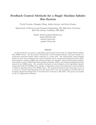
  • 34. 0 200 400 600 800 1000 0 0.01 0.02 0.03 0.04 0.05 0.06 0.07 0.08 0.09 0.1 Γ 1 (TestSignal1) time (sec) Figure 4.1: Plot of Γ1 (Test Signal 1) vs time 0 200 400 600 800 1000 0 0.005 0.01 0.015 0.02 0.025 0.03 0.035 0.04 0.045 0.05 Γ 2 (TestSignal2) time (sec) Figure 4.2: Plot of Γ2 (Test Signal 2) vs time 4 Open Loop Input-Output Behavior of the Synchronous Generator and Turbine-Governor System In this section we observe the open loop input-output behavior of the truth model and the reduced order nonlinear model of the SMIB for test signals given in Figure 4.1 and Figure 4.2. The first control input VF of the truth model and the first control input EFD of the reduced order model are different. As given in Equation (10.41) the field voltage, VF , is related to excitation field emf, EFD, by the following expression VF = rF ωRkMF EFD =e15EFD (4.1) In the above expression, ωR = 1 p.u., and e15 = ( rF ωRkMF ). We first test the truth model and the reduced order nonlinear model of the SMIB for Γ1 (Test signal 1) given in Figure 4.1. In this case the two inputs for the truth model are, u = [VF , uT ]T = [e15Γ1, Γ1]T, and the two inputs for the reduced order nonlinear model are, u = [EFD, uT ]T = [Γ1, Γ1]T. 34
  • 35. Figure 4.3, Figure 4.4, and Figure 4.5 show generator terminal voltage Vt, rotor angle δ, and frequency ω vs time plots for Γ1 (Test Signal 1) applied to the reduced order nonlinear model. From Figure 4.3 we can see that after the addition of the fourth step of Γ1 (Test Signal 1) at 600 seconds, the generator terminal voltage Vt settles to a new steady state value of 0.83 p.u.. From Figure 4.4 we can see that the rotor angle δ first undergoes a large undershoot, followed by oscillations about 0.1 p.u. after the application of the second incremental step of Γ1 at 200 seconds, which is further followed by reduced oscillations about 0.3 p.u. after the application of the third step of Γ1 at 400 seconds, and finally after the application of the fourth and final step at 600 seconds the oscillations almost die out and the rotor angle δ settles to a value of 0.725 p.u.. Figure 4.5 shows that the frequency ω settles to its steady state value of 1 p.u. after the application of the fourth step at 600 seconds. Like the rotor angle δ, the oscillations of the frequency ω also decrease with the application of each incremental step. Figure 4.6, Figure 4.7, and Figure 4.8 show generator terminal voltage Vt, rotor angle δ, and frequency ω vs time plots for Γ1 (Test Signal 1) applied to the truth model. From Figure 4.6 we can see that the generator terminal voltage Vt converges very slowly to the new steady state value of 0.83 p.u.. From Figure 4.7 we can see that the rotor angle δ first undergoes a large undershoot after which it oscillates about 0.1 p.u., where the oscillations decay with time. Figure 4.8 shows that the frequency ω oscillates about its steady state value of 1 p.u.. We observe a peculiar difference between the performance of the reduced order nonlinear model and the truth model, for Γ1 (Test Signal 1). The addition of each incremental step of Γ1 after a fixed interval has a distinct effect on the amplitude and damping of the output oscillations for the reduced order nonlinear model, where a rapid decrease in the output oscillations is observed with the application of each step. Thus, we observe transitions in the output response at time instants when incremental steps of Γ1 are applied to the reduced order nonlinear model. However, for the truth model, the effect of adding incremental steps at regular intervals is negligible on the output response, compared to the reduced order nonlinear model. We do not see transitions in the output behavior at time instants when incremental steps of Γ1 are applied to the truth model, and the oscillations decay more uniformly in this case. 35
  • 36. 0 200 400 600 800 1000 0.75 0.8 0.85 0.9 0.95 1 1.05 1.1 1.15 1.2 Generatorterminalvoltagevt(p.u.) time (sec) Figure 4.3: Plot of the generator terminal voltage Vt vs time for Γ1 (Test Signal 1) applied to the reduced order nonlinear model 0 200 400 600 800 1000 −1.5 −1 −0.5 0 0.5 1 delta(radians) time (sec) Figure 4.4: Plot of the rotor angle δ vs time for Γ1 (Test Signal 1) applied to the reduced order nonlinear model 0 200 400 600 800 1000 0.75 0.8 0.85 0.9 0.95 1 1.05 1.1 omega(radians/sec) time (sec) Figure 4.5: Plot of the frequency ω vs time for Γ1 (Test Signal 1) applied to the reduced order nonlinear model 36
  • 37. 0 200 400 600 800 1000 0.85 0.9 0.95 1 1.05 1.1 1.15 1.2 1.25 Generatorterminalvoltagevt(p.u.) time (sec) Figure 4.6: Plot of the generator terminal voltage Vt vs time for Γ1 (Test Signal 1) applied to the truth model 0 200 400 600 800 1000 −0.8 −0.6 −0.4 −0.2 0 0.2 0.4 0.6 0.8 1 delta(radians) time (sec) Figure 4.7: Plot of the rotor angle δ vs time for Γ1 (Test Signal 1) applied to the truth model 0 200 400 600 800 1000 0.98 0.985 0.99 0.995 1 1.005 1.01 1.015 omega(radians/sec) time (sec) Figure 4.8: Plot of the angular velocity ω vs time for Γ1 (Test Signal 1) applied to the truth model 37
  • 38. We now test the truth model and the reduced order nonlinear model of the SMIB for Γ2 (Test signal 2) given in Figure 4.2. In this case the two inputs for the truth model are, u = [VF , uT ]T = [e15Γ2, Γ2]T, and the two inputs for the reduced order nonlinear model are, u = [EFD, uT ]T = [Γ2, Γ2]T. Figure 4.9, Figure 4.10, and Figure 4.11 show generator terminal voltage Vt, rotor angle δ, and frequency ω vs time plots for Γ2 (Test Signal 2) applied to the reduced order nonlinear model. From Figure 4.9 we can see that the generator terminal voltage Vt settles to a new steady value of 0.82 p.u.. From Figure 4.10 we can see that the rotor angle δ first undergoes a large undershoot after which it oscillates about 0.1 p.u.. Figure 4.11 shows that the frequency ω oscillates about its steady state value of 1 p.u.. The oscillations decay with time. For Γ2 (Test Signal 2) where the magnitudes of the incremental steps are reduced to half of Γ1 (Test Signal 1), the effect of adding incremental steps of Γ2 after regular intervals to the reduced order nonlinear model, is not as significant as compared to the effect of Γ1 (Test Signal 1). The oscillations decay uniformly with time, and we do not see the sharp transitions that we saw when Γ1 was applied to the reduced order nonlinear model. Figure 4.12, Figure 4.13, and Figure 4.14 show generator terminal voltage Vt, rotor angle δ, and frequency ω vs time plots for Γ2 (Test Signal 2) applied to the truth model. These results are similar to the results obtained when Γ1 (Test Signal 1) is applied to the truth model. 38
  • 39. 0 200 400 600 800 1000 0.75 0.8 0.85 0.9 0.95 1 1.05 1.1 1.15 1.2 Generatorterminalvoltagevt(p.u.) time (sec) Figure 4.9: Plot of the generator terminal voltage Vt vs time for Γ2 (Test Signal 2) applied to the reduced order nonlinear model 0 200 400 600 800 1000 −1.5 −1 −0.5 0 0.5 1 delta(radians) time (sec) Figure 4.10: Plot of the rotor angle δ vs time for Γ2 (Test Signal 2) applied to the reduced order nonlinear model 0 200 400 600 800 1000 0.75 0.8 0.85 0.9 0.95 1 1.05 1.1 omega(radians/sec) time (sec) Figure 4.11: Plot of the frequency ω vs time for Γ2 (Test Signal 2) applied to the reduced order nonlinear model 39
  • 40. 0 200 400 600 800 1000 0.85 0.9 0.95 1 1.05 1.1 1.15 1.2 1.25 Generatorterminalvoltagevt(p.u.) time (sec) Figure 4.12: Plot of the generator terminal voltage Vt vs time for Γ2 (Test Signal 2) applied to the truth model 0 200 400 600 800 1000 −0.8 −0.6 −0.4 −0.2 0 0.2 0.4 0.6 0.8 1 delta(radians) time (sec) Figure 4.13: Plot of the rotor angle δ vs time for Γ2 (Test Signal 2) applied to the truth model 0 200 400 600 800 1000 0.98 0.985 0.99 0.995 1 1.005 1.01 1.015 omega(radians/sec) time (sec) Figure 4.14: Plot of the angular velocity ω vs time for Γ2 (Test Signal 2) applied to the truth model 40
  • 41. 5 The Decoupled Reduced Order Model Let us recall from the first section that small changes in real power are mainly dependent on changes in rotor angle δ, and thus the frequency (i.e. on the prime mover valve control), whereas the reactive power is mainly dependent on the voltage magnitude (i.e. on the generator excitation). The excitation system time constant is much smaller than the prime mover time constant and its transient decay much faster and does not affect the load frequency control (LFC) dynamics. Thus, the cross-coupling between the LFC loop and the automatic voltage regulator (AVR) loop is negligible. Hence, load frequency control and excitation voltage control can be analyzed independently. Therefore, we decouple the two-input two-output (MIMO) reduced order system into two single input single output (SISO) subsystems. The first SISO subsystem consists of the LFC loop, where the turbine valve control uT controls the rotor angle δ and thus the frequency ω of the synchronous generator. The second SISO subsystem consists of the AVR loop, where the generator excitation EFD controls the terminal voltage Vt of the synchronous generator. From Equation (3.59) and Equation (3.60) the linear model of the synchronous generator and turbine connected to an infinite bus is ∆ ˙E′ q = f11∆E′ q + ∂f1 ∂x3 x0 ∆δ + g11∆EFD ∆ ˙ω = ∂f2 ∂x1 x0 ∆E′ q + f27∆ω + ∂f2 ∂x3 x0 ∆δ + f28∆Tm ∆ ˙δ = ∆ω ∆ ˙Tm = f41∆Tm + f42∆GV ∆ ˙GV = f51∆ω + f52∆GV + g55∆uT (5.1) Note that all the coefficients in the above expression are evaluated at the nominal operating point given in the previous section. Let us denote ∂f1 ∂x3 x0 = A13 ∂f2 ∂x1 x0 = A21 ∂f2 ∂x3 x0 = A23 (5.2) The MIMO system with control inputs ∆EFD and ∆uT can be decoupled into the LFC loop with control input ∆uT as ∆ ˙ω = A21∆E′ q + f27∆ω + A23∆δ + f28∆Tm ∆ ˙δ = ∆ω ∆ ˙Tm = f41∆Tm + f42∆Gv ∆ ˙GV = f51∆ω + f52∆GV + g55∆uT (5.3) and the AVR loop with control input ∆EFD as ∆ ˙E′ q = f11∆E′ q + A13∆δ + g11∆EFD (5.4) The weak coupling A21∆E′ q between the LFC and the AVR loop can be neglected in the LFC loop in Equation (5.3), and the weak coupling A13∆δ between the LFC and the AVR loop can be neglected in the AVR loop in Equation (5.4). Neglecting theses terms, the LFC loop with control input ∆uT is approximated as ∆ ˙ω = f27∆ω + A23∆δ + f28∆Tm ∆ ˙δ = ∆ω ∆ ˙Tm = f41∆Tm + f42∆Gv ∆ ˙GV = f51∆ω + f52∆GV + g55∆uT (5.5) 41
  • 42. and the AVR loop with control input ∆EFD is approximated as ∆ ˙E′ q = f11∆E′ q + g11∆EFD (5.6) 5.1 LFC Dynamics In this section we present the dynamics of the (LFC) SISO system with control input ∆uT . We then perform root locus analysis of the uncompensated (LFC) SISO system. A PID controller is designed next to stabilize the (LFC) SISO system which is originally unstable. From Equation (5.5) the LFC dynamics are ∆ ˙ω = f27∆ω + A23∆δ + f28∆Tm ∆ ˙δ = ∆ω ∆ ˙Tm = f41∆Tm + f42∆Gv ∆ ˙GV = f51∆ω + f52∆GV + g55∆uT (5.7) Differentiating ∆ ˙ω and substituting ∆ ˙δ = ∆ω we have ∆¨ω = f27∆ ˙ω + A23∆ω + f28∆ ˙Tm (5.8) Taking the Laplace transform of Equation (5.8) with zero initial conditions we get s2 ∆ω(s) = f27s∆ω(s) + A23∆ω(s) + f28s∆Tm(s) (5.9) On rearranging Equation (5.9) and taking the Laplace transform of ∆ ˙δ = ∆ω ∆ω(s) ∆Tm(s) = f28s s2 − f27s − A23 ∆δ(s) ∆ω(s) = 1 s (5.10) Equation (5.10) evaluated at the nominal operating point gives ∆ω(s) ∆Tm(s) = 0.211s s2 + 0.3054 ∆δ(s) ∆ω(s) = 1 s (5.11) The dynamics of the turbine from Equation (5.7) can be written as ∆ ˙Tm = f41∆Tm + f42∆Gv (5.12) Taking the Laplace transform of Equation (5.12) with zero initial conditions s∆Tm(s) = f41∆Tm(s) + f42∆GV (s) (5.13) Rearranging and expressing Equation (5.13) as a transfer function ∆Tm(s) ∆GV (s) = f42 s − f41 (5.14) Equation (5.14) evaluated at the nominal operating point gives ∆Tm(s) ∆GV (s) = 2 s + 2 (5.15) 42
  • 43. u_T(s) delta(s) g55 s−f52 −f51 s−f52 f42 s−f41 f28.s s −f27s−A232 Step 1 sTm(s) omega(s) omega(s)Gv(s) delta(s) Figure 5.1: Simulink model of the (LFC) SISO system for a step input u_T(s) delta(s) g55 s−f52 −f51 g55 f42 s−f41 f28.s s −f27s−A232 Step 1 sTm(s) omega(s) omega(s) delta(s)Gv(s) Figure 5.2: Simulink model of the (LFC) SISO system for a step input From Equation (5.7) the governor dynamics can be written as ∆ ˙GV = f51∆ω + f52∆GV + g55∆uT (5.16) Taking the Laplace transform of Equation (5.16) with zero initial conditions s∆GV (s) = f51∆ω(s) + f52∆GV (s) + g55∆uT (s) (5.17) Rearranging and expressing Equation (5.17) as a transfer function ∆GV (s) = f51 s − f52 ∆ω(s) + g55 s − f52 ∆uT (s) (5.18) Equation (5.18) evaluated at the nominal operating point gives ∆GV (s) = −0.25 s + 5 ∆ω(s) + 5 s + 5 ∆uT (s) (5.19) Figure 5.1 shows the simulink block diagram of the LFC loop for a step input. In all simulink models the subscript ∆ is omitted for convenience. By moving the summing point ahead of the block g55 s−f52 , the simulink model in Figure 5.1 can be simplified to get the simulink model shown in Figure 5.2. In Figure 5.2 let G(s) = g55 s − f52 f42 s − f41 f28s s2 − f27s − A23 = g55f42f28s (s − f52)(s − f41)(s2 − f27s − A23) (5.20) and H(s) = − f51 g55 (5.21) Using Equation (5.20) and Equation (5.21), the simulink model in Figure 5.2 can be simplified to the simulink model shown in Figure 5.3. The open loop transfer function of the SISO system shown in Figure 5.3 with output ω(s) and step input uT (s) is G(s)H(s) = − f42f28f51s (s − f52)(s − f41)(s2 − f27s − A23) (5.22) 43
  • 44. Figure 5.3: Simulink model of the (LFC) SISO system for a step input The closed loop transfer function of the SISO system between the output ∆δ(s) and control input ∆uT (s) is ∆δ(s) ∆uT (s) = G(s) 1 + G(s)H(s) 1 s = g55f42f28 (s−f52)(s−f41)(s2−f27s−A23) 1 − f42f28f51s (s−f52)(s−f41)(s2−f27s−A23) = g55f42f28 (s − f52)(s − f41)(s2 − f27s − A23) − f51f42f28s (5.23) For a step input, ∆uT (s) = 1 s . From the final value theorem, the steady state value of ∆δ(s) is ∆δss = lim s→0 s∆δ(s) = lim s→0 s∆uT (s) g55f42f28 (s − f52)(s − f41)(s2 − f27s − A23) − f51f42f28s = − g55f42f28 f52f41A23 (5.24) Substituting numerical values for the constant parameters in Equation (5.24) we get ∆δss = 0.6909 (5.25) Also ∆ω(s) ∆uT (s) = G(s) 1 + G(s)H(s) = g55f42f28s (s−f52)(s−f41)(s2−f27s−A23) 1 − f42f28f51s (s−f52)(s−f41)(s2−f27s−A23) = g55f42f28s (s − f52)(s − f41)(s2 − f27s − A23) − f51f42f28s (5.26) From the final value theorem, the steady state value of ∆ω(s) for a step input is ∆ωss = lim s→0 s∆ω(s) = lim s→0 s∆uT (s) g55f42f28s (s − f52)(s − f41)(s2 − f27s − A23) − f51f42f28s = − lim s→0 g55f42f28 f52f41A23 s = 0 (5.27) Figure 5.4 and Figure 5.5 show the plots of ∆δ(s) and ∆ω(s) vs time for the uncompensated (LFC) SISO system for a step input, respectively. From these plots we can see that ∆δ(s) settles to a steady state value of 0.6909 and ∆ω(s) settles to a steady state value of 0 which are in agreement with the respective steady state values calculated in Equation (5.25) and Equation (5.27). Also the root locus plot in Figure 5.6 clearly shows that the uncompensated (LFC) SISO system with step input uT (s) is unstable. 44
  • 45. 0 100 200 300 400 500 600 700 800 900 1000 −0.2 0 0.2 0.4 0.6 0.8 1 1.2 1.4 ∆δ(radians) time (sec) Figure 5.4: Plot of ∆δ(s) vs time for the uncompensated (LFC) SISO system for a step input 0 100 200 300 400 500 600 700 800 900 1000 −0.4 −0.3 −0.2 −0.1 0 0.1 0.2 0.3 0.4 ∆ω(radians/sec) time (sec) Figure 5.5: Plot of ∆ω(s) vs time for the uncompensated (LFC) SISO system for a step input −20 −15 −10 −5 0 5 −15 −10 −5 0 5 10 15 Root Locus Real Axis ImaginaryAxis Figure 5.6: Root locus plot for the uncompensated (LFC) SISO system 45
  • 46. u_T(s) delta(s) g55 s−f52 −f51 g55 f42 s−f41 f28.s s −f27s−A232 PID Controller PID(s) 1 s 0 Tm(s) omega(s) omega(s) delta(s)Gv(s) e_T(s) Figure 5.7: Simulink model of the PID compensated (LFC) SISO system 5.1.1 PID controller design for the LFC loop In order to stabilize this system we design a proportional-integral-derivative (PID) controller. The simulink model of the PID compensated (LFC) SISO system is given in Figure 5.7. The output of the PID controller ∆uT (s) in the frequency domain is given by ∆uT (s) = Kp1∆eT (s) + Ki1 s ∆eT (s) + Kd1s∆eT (s) (5.28) where Kp1 is the proportional gain, Ki1 is the integral gain, Kd1 is the derivative gain, and ∆eT (s) is the error signal. Expressing Equation (5.28) as a transfer function ∆uT (s) ∆eT (s) = Kp1 + Ki1 s + Kd1s = Kd1s2 + Kp1s + Ki1 s (5.29) From Figure 5.7 the open loop transfer function of the PID compensated (LFC) SISO system can be written as GPID1(s) = Kd1s2 + Kp1s + Ki1 s G(s) 1 + G(s)H(s) = Kd1s2 + Kp1s + Ki1 s g55f42f28s (s − f52)(s − f41)(s2 − f27s − A23) − f51f42f28s HPID1(s) = 1 ∴ GPID1(s)HPID1(s) = Kd1s2 + Kp1s + Ki1 s g55f42f28s (s − f52)(s − f41)(s2 − f27s − A23) − f51f42f28s (5.30) The PID gains are tuned to Kp1 = 200, Ki1 = 150, and Kd1 = 100. Substituting these PID gains and numerical values for the constant coefficients in Equation (5.30) we get GPID1(s)HPID1(s) = 52.74s3 + 105.5s2 + 79.11s 5s5 + 35s4 + 51.53s3 + 10.69s2 + 15.27s (5.31) Figure 5.8 and Figure 5.9 show the plots for ∆δ(s) and ∆ω(s) vs time for the PID compensated (LFC) SISO system, respectively. Also, Figure 5.10 shows the root locus plot for the PID compensated (LFC) SISO system. From this plot it is evident that the PID compensated (LFC) SISO system is stable since the root locus lies entirely in the left half s-plane. 46
  • 47. 0 5 10 15 20 25 30 35 40 45 50 0 1 2 3 4 5 6 7 x 10 −5 ∆δ(radians) time (sec) Figure 5.8: Plot of ∆δ(s) vs time for the PID compensated (LFC) SISO system 0 5 10 15 20 25 30 35 40 45 50 −0.5 0 0.5 1 1.5 2 2.5 3 3.5 4 x 10 −5 ∆ω(radians/sec) time (sec) Figure 5.9: Plot of ∆ω(s) vs time for the PID compensated (LFC) SISO system −6 −5 −4 −3 −2 −1 0 1 −10 −8 −6 −4 −2 0 2 4 6 8 10 Root Locus Real Axis ImaginaryAxis Figure 5.10: Root locus plot for the PID compensated (LFC) SISO system 47
  • 48. 5.2 AVR Dynamics In this section we present the dynamics of the (AVR) SISO system with control input ∆EFD. In addition we also design a PID controller for the (AVR) SISO system. From Equation (5.6) the dynamics of the (AVR) SISO system are ∆ ˙E′ q = f11∆E′ q + g11∆EFD (5.32) Taking the Laplace transform of Equation (5.32) assuming zero initial conditions we get s∆E′ q(s) = f11∆E′ q(s) + g11∆EFD(s) (5.33) Rearranging and expressing Equation (5.33) as a transfer function ∆E′ q(s) ∆EFD(s) = g11 s − f11 (5.34) From Equation (3.71) the output terminal voltage ∆Vt is ∆Vt = T1∆E′ q + T2∆δ (5.35) For the decoupled (AVR) SISO system with ∆EFD as the input and ∆Vt as the output the coupling T2∆δ between the (LFC) SISO system and the (AVR) SISO system is neglected. Therefore, ∆Vt = T1∆E′ q (5.36) Taking the Laplace transform of Equation (5.36) ∆Vt(s) = T1∆E′ q(s) (5.37) Combining Equation (5.34) and Equation (5.37) we get ∆Vt(s) ∆EFD(s) = T1g11 s − f11 (5.38) Substituting numerical values for the coefficients in Equation (5.38) evaluated at the nominal operating point we get ∆Vt(s) ∆EFD(s) = 0.08913 s + 0.5517 (5.39) Figure 5.11 shows the simulink model of the uncompensated (AVR) SISO system for a step input. In Figure 5.11 let G1(s) = T1g11 s − f11 (5.40) and H1(s) = 1 (5.41) Therefore, the open loop transfer function of the uncompensated (AVR) SISO system shown in Figure 5.11 is G1(s)H1(s) = T1g11 s − f11 (5.42) The closed loop transfer function of the uncompensated (AVR) SISO system shown in Figure 5.11 is ∆Vt(s) ∆Eref (s) = G1(s) 1 + G1(s)H1(s) = T1g11 s−f11 1 + T1g11 s−f11 = T1g11 s − f11 + T1g11 (5.43) 48
  • 49. V_t T1*g11 s−f11Step V_t(s) E_ref E_FD(s) Figure 5.11: Simulink model of the uncompensated (AVR) SISO system for a step input For a step input, ∆Eref (s) = 1 s . From the final value theorem, the steady state value of ∆Vt(s) is ∆Vt(ss) = lim s→0 s∆Vt(s) = lim s→0 s∆Eref (s) T1g11 s − f11 + T1g11 = T1g11 T1g11 − f11 (5.44) Substituting numerical values for the coefficients in Equation (5.44) ∆Vt(ss) = 0.1391 (5.45) Figure 5.12 shows the terminal voltage ∆Vt(s) vs time plot for the uncompensated (AVR) SISO system for a step input. From this plot we can see that ∆Vt(s) settles to a steady state value of 0.1391 which is in agreement with the steady state value calculated in Equation (5.45). Figure 5.13 shows the root locus plot for the uncompensated (AVR) SISO system. From this plot it is evident that the uncompensated (AVR) SISO system is stable. 49
  • 50. 0 5 10 15 20 25 30 35 40 45 50 0 0.02 0.04 0.06 0.08 0.1 0.12 0.14 0.16 Generatorterminalvoltage∆V t (p.u.) time (sec) Figure 5.12: Plot of the terminal voltage ∆Vt(s) vs time for the uncompensated (AVR) SISO system for a step input −2 −1.5 −1 −0.5 0 0.5 −0.08 −0.06 −0.04 −0.02 0 0.02 0.04 0.06 0.08 Root Locus Real Axis ImaginaryAxis Figure 5.13: Root locus plot for the uncompensated (AVR) SISO system 5.2.1 PID controller design for the AVR loop We design a PID controller to improve the transient and steady state response of the (AVR) SISO system. The output of this PID controller ∆EFD(s) in the frequency domain is given by ∆EFD(s) = Kp2∆eFD(s) + Ki2 s ∆eFD(s) + Kd2s∆eFD(s) (5.46) where Kp2 is the proportional gain, Ki2 is the integral gain, Kd2 is the derivative gain, and ∆eFD(s) is the error signal. Expressing Equation (5.46) as a transfer function ∆EFD(s) ∆eFD(s) = Kp2 + Ki2 s + Kd2s = Kd2s2 + Kp2s + Ki2 s (5.47) 50
  • 51. V_T(s) T1*g11 s−f11 PID Controller PID(s) 0 V_T(s)e_FD(s) E_FD(s) Figure 5.14: Simulink model of the PID compensated (AVR) SISO system 0 5 10 15 20 25 30 35 40 45 50 −0.5 0 0.5 1 1.5 2 2.5 3 3.5 4 x 10 −4 Generatorterminalvoltage∆Vt (p.u.) time (sec) Figure 5.15: Plot of ∆Vt(s) vs time for the PID compensated (AVR) SISO system −1.4 −1.2 −1 −0.8 −0.6 −0.4 −0.2 0 0.2 −1.5 −1 −0.5 0 0.5 1 1.5 Root Locus Real Axis ImaginaryAxis Figure 5.16: Root locus plot for the PID compensated (AVR) SISO system From Figure 5.14 the open loop transfer function of the PID compensated (AVR) SISO system can be written as GPID2(s) = Kd2s2 + Kp2s + Ki2 s T1g11 s − f11 HPID2(s) = 1 ∴ GPID2(s)HPID2(s) = Kd2s2 + Kp2s + Ki2 s T1g11 s − f11 (5.48) The PID gains Kp2 = 10, Ki2 = 10, and Kd2 = 4 are tuned so as to get the best system response. Substituting these PID gains and numerical values for the constant coefficients in Equation (5.48) we get GPID2(s)HPID2(s) = 0.3565s2 + 0.8913s + 0.8913 s2 + 0.5517s (5.49) Figure 5.15 shows the generator terminal voltage ∆Vt(s) vs time plot for the PID compensated (AVR) SISO system. From this plot we can see that ∆Vt(s) attains its steady state value of 0 in approximately 10 seconds. Figure 5.16 shows the root locus plot for the PID compensated (AVR) SISO system. The PID compensated (AVR) SISO system is stable since the root locus lies in the left half s-plane. 51
  • 52. 5.3 LFC and AVR including coupling As there is weak coupling between the LFC and AVR subsystems, the rotor angle δ and thus the frequency ω, and the terminal voltage Vt were controlled separately. In this section we study the effect of coupling between the LFC and the AVR system. In the previous section we saw that the weak coupling A21∆E′ q between the LFC and the AVR loop which appeared in the coupled system in Equation (5.1) was neglected in the LFC loop in Equation (5.5). Also, the weak coupling A13∆δ between the LFC and the AVR loop which appeared in the coupled system in Equation (5.1) was neglected in the AVR loop in Equation (5.6). In the coupled system including the LFC and AVR dynamics we do not neglect these terms. Thus, from Equation (5.1) we can write ∆ ˙E′ q = f11∆E′ q + A13∆δ + g11∆EFD ∆ ˙ω = A21∆E′ q + f27∆ω + A23∆δ + f28∆Tm ∆ ˙δ = ∆ω (5.50) Taking the Laplace transform of the expression for ∆ ˙E′ q in Equation (5.50) s∆E′ q(s) = f11∆E′ q(s) + A13∆δ(s) + g11∆EFD(s) (5.51) Rearranging Equation (5.51) we get ∆E′ q(s) = A13 s − f11 ∆δ(s) + g11 s − f11 ∆EFD(s) (5.52) Also from Equation (3.71) the first output which is the terminal voltage Vt of the synchronous generator for the coupled system including LFC and AVR dynamics is ∆Vt = T1∆E′ q + T2∆δ (5.53) The Laplace transform of Equation (5.53) gives ∆Vt(s) = T1∆E′ q(s) + T2∆δ(s) (5.54) Next, taking the derivative of ∆ ˙ω we get ∆¨ω = A21∆ ˙E′ q + f27∆ ˙ω + A23∆ω + f28∆ ˙Tm (5.55) Taking the Laplace transform of Equation (5.55) s2 ∆ω(s) = A21s∆E′ q(s) + f27s∆ω(s) + A23∆ω(s) + f28s∆Tm(s) (5.56) Rearranging Equation (5.56) we get ∆ω(s) = A21s s2 − f27s − A23 ∆E′ q(s) + f28s s2 − f27s − A23 ∆Tm(s) (5.57) Also the Laplace transform of ∆ ˙δ = ∆ω is s∆δ(s) = ∆ω(s). Thus, the second output which is the rotor angle ∆δ(s) of the synchronous generator for the coupled system including the LFC and AVR dynamics can be written as ∆δ(s) = A21 s2 − f27s − A23 ∆E′ q(s) + f28 s2 − f27s − A23 ∆Tm(s) (5.58) 52
  • 53. omega(s) delta(s) V_T(s) A13 s−f11 A21.s s −f27s−A232 g55 s−f52 g11 s−f11 −f51 g55 f42 s−f41 f28.s s −f27s−A232 T2 T2 T1 T1 PID Controller 2 PID(s) PID Controller 1 PID(s) 1 s 0 0 E_FD(s) Tm(s) u_T(s) omega(s) Eq_p(s) V_T(s) Gv(s) Figure 5.17: Simulink model of the PID compensated (LFC+AVR) MIMO system including coupling 6 PID Controller Design 6.1 PID Controller Design based on linear model The two PID controllers that were designed for the LFC and the AVR SISO systems in the previous section, are now tested on the combined LFC and AVR system including coupling which is the same as the linear model. A simulink block diagram which consists of the two PID controllers and the combined LFC and AVR system including coupling is constructed in Figure 5.17. Figure 6.1 to Figure 6.5 show ∆δ(s), ∆ω(s), ∆Vt(s), ∆Efd(s), and ∆uT (s) vs time plots for the PID compensated combined (LFC+AVR) MIMO system including coupling. The plots obtained when the coupling coefficients were set to zero i.e. in the decoupled LFC and AVR SISO systems, are identical to the plots obtained for the combined (LFC+AVR) MIMO system including coupling. Thus, separate frequency and voltage control of the synchronous generator and turbine-governor system connected to an infinite bus is justified. 53