Table 2: Survival Status Disease Severity Donor’s Sex Alive Dead Total None Female 14 1 15 Male 21 2 23 Mild Female 17 1 18 Male 40 2 42 Moderate Female 15 1 16 Male 33 6 39 Severe Female 6 1 7 Male 16 17 33 Total 162 31 193 2. Using data in table 2, compute the common odds ratio of the association between donor’s sex and the survival status of the infant, after controlling for severity ?. A)Manually calculate a common odds ratio to test the hypothesis of no association between donor’s sex and the survival status of the infant, after the inclusion of the variable severity using the common odds ratio? B)Interpret the results. How does the common odds ratio differ from the simple odds ratio computed in part 1? What effect might it have on your decision from part 1 to reject or fail to reject the null hypothesis? C)Why is it important to know the effect of severity on the association of gender and survival? 3. Perform a simple logistic regression using SPSS and the Wk 6 Dataset (SPSS document). Answer the following questions based on your SPSS output A)Are the results of the simple logistic regression similar to or different from the results of the simple odds ratio ? B)How are they similar or different? Include output from SPSS and an interpretation of the OR and confidence intervals in your response? C)What can you do using logistic regression to duplicate the results from part 2 of this application (the use of CMH for common odds) ? Answer question 1 using data in table 1 below. Table 1: Survival Status Donor’s Sex Alive Dead Total Female 52 4 56 Male 110 27 137 Total 162 31 193 1. Compute the simple odds ratio of the association of donor’s sex and survival status of the infant. Be sure to answer all four parts to this question (a, b, c, and d), including manual calculation of the chi-square value. A)Manually calculate a simple odds ratio to test the hypothesis of no association between donor’s sex and the survival status of the infant, without the inclusion of the variable severity using a 2 x 2 table for sex and survival B)Manually calculate the confidence interval associated with that odds ratio using the appropriate formula C)Manually compute the Chi Square test statistic for this table 1. Interpret the results. Include an interpretation of the odds ratio, the confidence interval, and the Chi Square test statistic in your response PART3 Step-by-Step Guide to Assignment 6.3 Odds Ratios Problem 3. Perform a simple logistic regression using SPSS and the practice problem 6.3 data set. Answer the following questions based on your SPSS output Step 1. Open the practice_problem_6.3.sav dataset. Step 2. Go to Analyze ( Regression ( Binary logistic Step 3. Place Survival_Status in the Dependent box and place Gender in the Covariate(s) box. Click Options. Step 4. In the Logistic Regression: Options window, check Classification plots, Casewise listing of residuals, and CI for exp(B)..

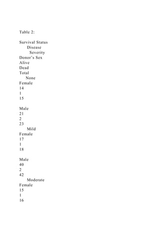
1. Table 2:
Survival Status
Disease
Severity
Donor’s Sex
Alive
Dead
Total
None
Female
14
1
15
Male
21
2
23
Mild
Female
17
1
18
Male
40
2
42
Moderate
Female
15
1
16

2. Male
33
6
39
Severe
Female
6
1
7
Male
16
17
33
Total
162
31
193
2. Using data in table 2, compute the common odds ratio of the
association between donor’s sex and the survival status of the
infant, after controlling for severity ?.
A)Manually calculate a common odds ratio to test the
hypothesis of no association between donor’s sex and the
survival status of the infant, after the inclusion of the variable
severity using the common odds ratio?
B)Interpret the results. How does the common odds ratio differ
from the simple odds ratio computed in part 1? What effect
might it have on your decision from part 1 to reject or fail to
reject the null hypothesis?
C)Why is it important to know the effect of severity on the
association of gender and survival?
3. Perform a simple logistic regression using SPSS and the Wk
6 Dataset (SPSS document). Answer the following questions
based on your SPSS output

3. A)Are the results of the simple logistic regression similar to or
different from the results of the simple odds ratio ?
B)How are they similar or different? Include output from SPSS
and an interpretation of the OR and confidence intervals in your
response?
C)What can you do using logistic regression to duplicate the
results from part 2 of this application (the use of CMH for
common odds) ?
Answer question 1 using data in table 1 below.
Table 1:
Survival Status
Donor’s Sex
Alive
Dead
Total
Female
52
4
56
Male
110
27
137
Total
162
31
193
1. Compute the simple odds ratio of the association of donor’s
sex and survival status of the infant. Be sure to answer all four
parts to this question (a, b, c, and d), including manual
calculation of the chi-square value.
A)Manually calculate a simple odds ratio to test the hypothesis

4. of no association between donor’s sex and the survival status of
the infant, without the inclusion of the variable severity using a
2 x 2 table for sex and survival
B)Manually calculate the confidence interval associated with
that odds ratio using the appropriate formula
C)Manually compute the Chi Square test statistic for this table
1. Interpret the results. Include an interpretation of the odds
ratio, the confidence interval, and the Chi Square test statistic
in your response
PART3
Step-by-Step Guide to Assignment 6.3
Odds Ratios
Problem 3. Perform a simple logistic regression using SPSS and
the practice problem 6.3 data set. Answer the following
questions based on your SPSS output
Step 1. Open the practice_problem_6.3.sav dataset.
Step 2. Go to Analyze ( Regression ( Binary logistic
Step 3. Place Survival_Status in the Dependent box and place
Gender in the Covariate(s) box. Click Options.
Step 4. In the Logistic Regression: Options window, check
Classification plots, Casewise listing of residuals, and CI for
exp(B). Make sure CI for exp(B) is set to 95%. Click Continue.
Click OK.
SPSS Output:
Case Processing Summary
Unweighted Casesa
N

5. Percent
Selected Cases
Included in Analysis
181
100.0
Missing Cases
0
.0
Total
181
100.0
Unselected Cases
0
.0
Total
181
100.0
a. If weight is in effect, see classification table for the total
number of cases.
The Case Processing Summary table shows there are 181 cases
in the data set and there are no missing data. It also shows the
percentages of cases represented in the regression analysis.
Dependent Variable Encoding
Original Value
Internal Value
ALIVE
0
DEAD
1
The Dependent Variable Encoding shows that SPSS has
numerically coded the two levels of survival status, which are
string variables in the data set. Alive = 0 and Dead = 1.
Categorical Variables Codings

6. Frequency
Parameter coding
(1)
Gender
FEMALE
53
1.000
MALE
128
.000
SPSS has also coded the Gender variable levels. The
Categorical Variables Codings table shows that the output will
provide the odds ratio of males to females.
The first set of Output after the above is Block 0 output:
Classification Tablea,b
Observed
Predicted
Survival_Status
Percentage Correct
ALIVE
DEAD
Step 0
Survival_Status
ALIVE
150
0

7. 100.0
DEAD
31
0
.0
Overall Percentage
82.9
a. Constant is included in the model.
b. The cut value is .500
Variables in the Equation
B
S.E.
Wald
df
Sig.
Exp(B)
Step 0
Constant
-1.577
.197
63.862
1
.000
.207
The two tables above (Classification Table and Variables in the
Equation table) reflect the predicted results of survival without
any independent variables included in the model. Block 0 is also
called the “constant only” model or the “reduced model”. It
serves as the baseline to which a regression model with
independent or predictor variables will be compared.

8. The second set of output is labeled Block 1:
Omnibus Tests of Model Coefficients
Chi-square
df
Sig.
Step 1
Step
5.506
1
.019
Block
5.506
1
.019
Model
5.506
1
.019
The Omnibus Test of Model Coefficients table compares the full
model to the baseline (Block 0) model. If the chi square
significance (p) value is <0.05, then the block 1 model is a
significantly better predictor than the Block 0 model.
In this problem, the significance value is 0.019, which is less
than 0.05, so the block 1 model is a significantly better
predictor than the Block 0 model.
Model Summary
Step
-2 Log likelihood
Cox & Snell R Square
Nagelkerke R Square
1
160.252a

9. .030
.050
a. Estimation terminated at iteration number 5 because
parameter estimates changed by less than .001.
Interpretation:
What is the meaning of R squares in model summary tables?
Variables in the Equation
B
S.E.
Wald
df
Sig.
Exp(B)
95% C.I.for EXP(B)
Lower
Upper
Step 1a
Gender(1)
-1.186
.563
4.434
1
.035
.305
.101
.921

10. Constant
-1.319
.217
37.081
1
.000
.267
a. Variable(s) entered on step 1: Gender.
The values of interest in the Variables in the Equation table are
the significance of the Wald, the Exp(B), and the 95%
Confidence Intervals for Exp(B). The Wald test is done to
determine if the predictor variable(s) make a significant
contribution to the model. A Sig. (p-value) of the Wald <0.05
indicates a significant contribution. Exp(B) is the odds ratio
(OR) for the independent variable. It provides the amount of
change in odds for the dependent variable resulting from a one
unit change in the independent variable or predictor variables.
An Exp(B) 0.0 to less than 1.0 indicates an inverse relationship
between the independent and the dependent variables. In this
problem, an Exp(B) <1.0 means less likely to survive than the
reference category.
An Exp(B) >1.0 indicates a positive relationship between the
independent and dependent variables. In our problem an Exp(B)
>1.0 means more likely to survive than the reference category.
Interpretation:
Your interpretation must cover the followings:
· Using data from the table to compare survival among males
and females
Identifying whether there is a significant association between
gender and survival based on the CI for gender in this model

11. a. Are the results of the simple logistic regression similar to or
different from the results of the simple odds ratio?
The OR from SPSS is the inverse of the OR calculated in
problem 6.1.
b. How are they similar or different? Include output from SPSS
and an interpretation of the OR and confidence intervals in your
response.
The OR hand calculated in problem 6.1 was 3.275 (95% CI
1.09, 9.88). This means that females are more than 3 times more
likely to survive than males. The OR calculated by SPSS =
0.305 (95% CI 0.10, 0.92). This means that males are about 30%
less likely to survive than females. The ORs are reversed.
The hand calculated OR in problem 6.1 compared males to
females. As noted earlier, SPSS selected males to be the
reference (male = 0) and females to be compared to males
(females = 1). This is why it is important to review the output
tables that describe how the data were coded by SPSS.
To replicate the results of problem 6.3 with the hand
calculation, we need to switch the referent group to males. This
is done by calculating 1 / OR for females or 1 / 3.275.
1 / 0.305 = 0.305
To calculate the 95% CI, we apply the same methodology, but
reverse the order so that 1 / lower 95% CI becomes the upper
95% CI and 1 / upper 95% CI becomes the lower 95% CI:
Upper limit is 9.88 in problem 6.1.
1 / 9.88 = 0.101
This becomes the lower limit for the 95% CI
Lower limit is 1.09 in problem 6.1.
1 / 1.09 = 0.92

12. This becomes the upper limit for the 95% CI
Thus, males are about 31% (OR 0.305; 95% CI 0.10, 0.92) less
likely to survive than females. The hand-calculated results now
duplicate the SPSS results.
c. What can you do using logistic regression to duplicate the
results from part 2 of this application (the use of CMH for
common odds)
To duplicate the results from part 2 of this application (the
common odds ratio), we would need to add the independent
variable disease severity to the independent variables box with
gender and conduct a multivariable logistic regression analysis.
PART2
Step-by-Step Guide to Assignment 6.2
This Step-by-Step Guide reviews how to manually calculate
common odds ratios (OR) and the confidence interval associated
with the OR, and interpret the results.
Problem 2. Compute the common odds ratio of the association
between donor’s sex and the survival status of the infant, after
controlling for severity.
2a. Manually calculate a common odds ratio to test the
hypothesis of no association between donor’s sex and the
survival status of the infant, after the inclusion of the variable
severity using the CMH test.
We begin with a multiple contingency table:
Survival Status
Disease Severity
Donor’s Sex
Alive
Dead
Total

13. None
Female
13
1
14
Male
19
2
21
Mild
Female
16
1
17
Male
37
2
39
Moderate
Female
14
1
15
Male
31
6
37
Severe
Female
6
1
7

14. Male
14
17
31
Total
150
31
181
In this table, there are four levels of disease severity (none,
mild, moderate, and severe) subdivided by each level of sex
(female and male). The dependent variable is dichotomous
(Survival level: alive and dead), which satisfies the assumption
for logistic regression.
Within this table there are four sub-tables from which four
separate odds ratios can be calculated: OR of survival by sex for
no disease, OR of survival by sex for mild disease, OR of
survival by sex for moderate disease, and OR of survival by sex
for severe disease. For CMH, the OR should be similar. Thus,
we calculate each OR to determine similarity.
We will use the “shortcut” for OR = (a * d) / (b * c)
Odd Ratios:
Survival between females and males with no disease:
= (13 * 2) / (1 * 19) = 1.368421
Survival between females and males with mild disease:
= (16 * 2) / (1 * 37) = 0.864865
Survival between females and males with moderate disease:
= (14 * 6) / (1 * 31) = 2.709677
Survival between females and males with severe disease:

15. = (6 * 17) / (1 * 14) = 7.285714
These are not really all in the same direction. The odds are
greater for survival in females with no disease, moderate
disease, and severe disease. However, the odds were lower in
females with mild disease than males. The concern is that the
common odds, which include all odds ratios, would mask this
inverse ratio because they are all combined.
For purposes of the assignment, we proceed with the calculation
of the common odds, bearing this in mind.
CMH formula for common odds ratio:
OR = Σ [ai (di / ni)] / Σ [bi (ci / ni)]
Using the data from the table:
Numerator
= [13 (2 / 35)] + [16 (2 / 56)] + [14 (6 / 52)] + [6 (17 / 38)]
= (0.742857) + (0.571429) + (1.615385) + (2.684211)
= 5.61388
Denominator = [1 (19 / 35)] + [1 (37 / 56)] + [1 (31 / 52)] + [1
(14 / 38)]
= (0.542857) + (0.660714) + (0.596154) + (0. 368421)

16. = 2.16815
Common OR = 5.61388 / 2.16815 = 2.59
Interpretation of results
2b. Interpret the results. How does the common odds ratio
differ from the simple odds ratio computed in part 1? What
effect might it have on your decision from part 1 to reject or
fail to reject the null hypothesis?
Based on the common odds ratio (OR), females are more than
twice (OR= 2.59) as likely to survive as males after controlling
for disease severity.
In the simple OR, females were more than 3 times (OR= 3.275)
as likely to survive than males. However, the simple OR
calculation considered only the odds of survival based on the
sex of the individual and did not account for disease severity.
In the common odds ratio (OR =2.59), we account for disease
severity by weighting the odds ratios according to the
proportion of the sample within each specific level of disease
severity. This means that disease severity is taken into account
in the calculation of the odds ratio. The common OR is lower
than the simple OR because disease severity plays a role in
survival in addition to sex.
Importance of knowing disease severity
2c. Why is it important to know the effect of severity on the
association of gender and survival?
In general, disease severity would affect the survival regardless
of gender. Less severe disease would likely have a bigger
chance of survival than more severe disease. Therefore when
assessing the association of gender and survival, it will be
important to consider the effect of disease severity. As shown in
the calculations for Part 2a, gender effect on the survival is not
same across the disease severity levels. Females without disease

17. or with moderate/severe disease were more likely to survive
than the male in the same disease status, males with mild
disease has a bigger odd of survival than female. Without
considering the severity of disease in males, simple OR will
overestimate the effect of sex on survival. Controlling for
disease severity, we see there is still an association between sex
and survival, but the association is substantially reduced.
However, ORs are very different across disease severity levels,
disease severity is an effect modifier. Therefore, we should
report OR for each disease severity instead of using simple OR
or common OR.
PART1
Step-by-Step Guide to Assignment 6.1
This Step-by-Step Guide shows how to manually calculate
simple odds ratios (OR), its confidence interval, and interpret
the results.
Problem 1. Compute the simple odds ratio of the association of
donor’s sex and survival status of the infant.
a. Manually calculate a simple odds ratio to test the hypothesis
of no association between donor’s sex and the survival status of
the infant, without the inclusion of the variable severity using a
2 x 2 table for sex and survival
Begin with a 2 x 2 table:
Donor’s sex
Survival status designated as Alive (yes) or Dead (Alive no)
Alive yes
Alive no
Female
a
b
All Exposed (a + b)
Male

18. c
d
All Not exposed (c + d)
Total
All Alive (a + c)
All Not Alive (b + d)
Total sample
Using the practice data set:
Donor’s sex
Survival status : Alive (Survived yes) or Dead (Survived no)
Alive yes
Alive no
Female
49
4
Total Female (53)
Male
101
27
Total Male (128)
Total
All Alive (150)
All Not Alive (31)
Total sample (181)
The formula for the odds ratio is the odds of death in females
divided by the odds of death in males. Using the letters from
the table:
OR= (a/b) ÷ (c/d) or with the numbers it is: (49/4)÷ (101/27) =
12.25÷.3.741 = 3.275
A common shortcut to this calculation is multiplying (a x d) and
then dividing this by (b x c) or [(ad)÷(bc)]
OR = 3.275
b. Manually calculate the confidence interval associated with

19. that odds ratio using the appropriate formula.
The formula for a 95% CI for an OR is e lnOR±z * SElnOR.
This means that the natural logarithm (base e) is used.
Step 1: Determine the natural logarithm (ln) for the odds ratio
(lnOR) using Excel or a scientific calculator.
OR= 3.275
ln(3.275) = 1.186242
(To verify the calculation: On the calculator enter: ln(3.275).
Your answer should be 1.186)
Step 2: Determine the standard error (SE).
Using the 2 x 2 table above,
SE= √ (1/a) + (1/b) + (1/c) + (1/d)
= √ (1/49) + (1/4) + (1/101) + (1/27)
= √ 0.020408163 + 0.25 + 0.00990099 + 0.037037037
= √ 0.317346
= 0.563335
Step 3: To calculate SE * z, multiply the SE by z for 95%
probability, which is 1.96. The confidence coefficient (z) is
from the standard normal distribution; 1.96 for a 95%
confidence interval.
SE * z = 0.563335 * 1.96 = 1.104136
Step 4: Complete calculating the exponent formula for both the
upper and lower limits:
Upper limit exponent:
= lnOR + SE (z)
= 1.186242 + 1.104136

20. = 2.290379
Lower limit exponent:
= lnOR – SE (1.96)
=1.186242 - 1.104136
=0.082106
Step 5 Calculate the final 95% CI limits using the exponent
function (EXP) in Excel:
Upper CI:
= e2.290379
= 9.87868
Lower CI:
= e0.082106
= 1.08557
Final results:
The lower 95% CI is 1.08557
The upper 95% CI is 9.87868
95% CI = (1.09, 9.88)
c. Manually compute the Chi Square test statistic for this table
(10 points).
The 2 x 2 contingency table for the Chi Square statistic is
estimated using the formula below:
χ2 = [(ad - bc)2 (a + b + c + d)] / (a + b)(c + d)(b + d)(a + c)
or
χ2 = [(ad - bc)2 (N)] / (a + b)(c + d)(b + d)(a + c)
2 x 2 Table

21. Health Status (e.g Survival Status)
Variable type (e.g. Donor’s Sex)
Data Type 1 (e.g. Alive)
Data type 2 (e.g. Dead)
Total
Female
a
b
a + b
Male
c
d
c + d
Total
a + c
b + d
a + b + c + d = N
Survival Status
Donor’s Sex
Alive
Dead
Total
Female
49
4
53
Male
101
27
128
Total
150
31
181
χ2 = [(ad - bc)2 (N)] / (a + b)(c + d)(b + d)(a + c)

22. = [(49 x 27 – 4 x 101)2(181)] / (53)(128)(31)(150)
= [(1323 – 404)2 (181)] / 31545600
= [(919)2(181)] / 31545600
= [(844561)(181)] / 31545600
= 152865541/31545600
= 4.846
The table calculated X2 value is 4.846.
d. Interpret the results. Include an interpretation of the odds
ratio and the confidence interval in your response (12 Points).
The odds ratio (OR) is 3.275. This means that females in this
sample are more than 3 (OR 3.28) times as likely to live than
males. However, the 95% confidence interval (95% CI 1.09,
9.88) is wide, indicating that In 95 out of 100 samples, the ratio
of odds can be as low as almost 1 (1.09) and nearly as high as
10 (9.88). The OR is statistically significant because the 95%
confidence interval does not include 1.0.
The wide confidence interval indicates the sample size was
relatively small. A larger sample size would narrow the
confidence interval.