ICVSS 2014 reading group

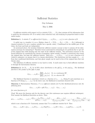
1. Sufficient Statistics
Guy Lebanon
May 2, 2006
A sufficient statistics with respect to θ is a statistic T(X1, . . . , Xn) that contains all the information that
is useful for the estimation of θ. It is useful a data reduction tool, and studying its properties leads to other
useful results.
Definition 1. A statistic T is sufficient for θ if p(x1, . . . , xn|T(x1, . . . , xn)) is not a function of θ.
A useful way to visualize it is as a Markov chain θ → T(X1, . . . , Xn) → {X1, . . . , Xn} (although in
classical statistics θ is not a random variable but a specific value). Conditioned on the middle part of the
chain, the front and back are independent.
As mentioned above, the intuition behind the sufficient statistic concept is that it contains all the infor-
mation necessary for estimating θ. Therefore if one is interested in estimating θ, it is perfectly fine to ‘get rid’
of the original data while keeping only the value of the sufficient statistic. The motivation connects to the
formal definition by considering the concept of sampling a ghost sample: Consider a statistician who erased
the original data, but kept the sufficient statistic. Since p(x1, . . . , xn|T(x1, . . . , xn)) is not a function of θ
(which is unknown), we assume that it is a known distribution. The statistician can then sample x1, . . . , xn
from that conditional distribution, and that ghost sample can be used in lieu of the original data that was
thrown away.
The definition of sufficient statistic is very hard to verify. A much easier way to find sufficient statistics
is through the factorization theorem.
Definition 2. Let X1, . . . , Xn be iid RVs whose distribution is the pdf fXi
or the pmf pXi
. The likelihood
function is the product of the pdfs or pmfs
L(x1, . . . , xn|θ) =
n
i=1 fXi (xi) Xi is a continuous RV
n
i=1 pXi
(xi) Xi is a discrete RV
.
The likelihood function is sometimes viewed as a function of x1, . . . , xn (fixing θ) and sometimes as a
function of θ (fixing x1, . . . , xn). In the latter case, the likelihood is sometimes denoted L(θ).
Theorem 1 (Factorization Theorem). T is a sufficient statistic for θ if the likelihood factorizes into the
following form
L(x1, . . . , xn|θ) = g(θ, T(x1, . . . , xn)) · h(x1, . . . , xn)
for some functions g, h.
Proof. We prove the theorem only for the discrete case (the continuous case requires different techniques).
First assume the likelihood factorizes as above. Then
p(x1, . . . , xn|T(x1, . . . , xn)) =
p(x1, . . . , xn, T(x1, . . . , xn))
p(T(x1, . . . , xn))
=
p(x1, . . . , xn)
y:T (y)=T (x) p(y1, . . . , yn)
=
h(x1, . . . , xn)
y:T (y)=T (x) h(y1, . . . , yn)
which is not a function of θ. Conversely, assume that T is a sufficient statistic for θ. Then
L(x1, . . . , xn|θ) = p(x1, . . . , xn|T(x1, . . . , xn), θ)p(T(x1, . . . , xn)|θ) = h(x1, . . . , xn)g(T(x1, . . . , xn), θ).
1

2. Example: A sufficient statistic for Ber(θ) is Xi since
L(x1, . . . , xn|θ) =
i
θxi
(1 − θ)1−xi
= θ
P
xi
(1 − θ)n−
P
xi
= g θ, xi · 1.
Example: A sufficient statistic for the uniform distribution U([0, θ]) is max(X1, . . . , Xn) since
L(x1, . . . , xn|θ) =
i
1
θ
·1{0≤xi≤θ} = θ−n
·1{max(x1,...,xn)≤θ}·1{min(x1,...,xn)≥0} = g(θ, max(x1, . . . , xn))h(x1, . . . , xn).
In the case that θ is a vector rather than a scalar, the sufficient statistic may be a vector as well. In this
case we say that the sufficient statistic vector is jointly sufficient for the parameter vector θ. The definitions
and factorization theorem carry over with little change.
Example: T = ( Xi, X2
i ) are jointly sufficient statistics for θ = (µ, σ2
) for normally distributed data
X1, . . . , Xn ∼ N(µ, σ2
):
L(x1, . . . , xn|θ) =
i
1
√
2πσ2
e−(xi−µ)2
/(2σ2
)
= (2πσ2
)−n/2
e−
P
i(xi−µ)2
/(2σ2
)
= (2πσ2
)−n/2
e−
P
i x2
i /(2σ2
)+2µ
P
i xi/(2σ2
)−µ2
/(2σ2
)
= g(θ, T) · 1 = g(θ, T) · h(x1, . . . , xn)
Clearly, sufficient statistics are not unique. From the factorization theorem it is easy to see that (i)
the identity function T(x1, . . . , xn) = (x1, . . . , xn) is a sufficient statistic vector and (ii) if T is a sufficient
statistic for θ then so is any 1-1 function of T. A function that is not 1-1 of a sufficient statistic may or may
not be a sufficient statistic. This leads to the notion of a minimal sufficient statistic.
Definition 3. A statistic that is a sufficient statistic and that is a function of all other sufficient statistics
is called a minimal sufficient statistic.
In a sense, a minimal sufficient statistic is the smallest sufficient statistic and therefore it represents the
ultimate data reduction with respect to estimating θ. In general, it may or may not exists.
Example: Since T = ( Xi, X2
i ) are jointly sufficient statistics for θ = (µ, σ2
) for normally distributed
data X1, . . . , Xn ∼ N(µ, σ2
), then so are ( ¯X, S2
) which are a 1-1 function of ( Xi, X2
i ).
The following theorem provides a way of verifying that a sufficient statistic is minimal.
Theorem 2. T is a minimal sufficient statistics if
L(x1, . . . , xn|θ)
L(y1, . . . , yn|θ)
is not a function of θ ⇔ T(x1, . . . , xn) = T(y1, . . . , yn).
Proof. First we show that T is a sufficient statistic. For each element in the range of T, fix a sample
yt
1, . . . , yt
n. For arbitrary x1, . . . , xn denote T(x1, . . . , xn) = t and
L(x1, . . . , xn|θ) =
L(x1, . . . , xn|θ)
L(yt
1, . . . , yt
n|θ)
L(yt
1, . . . , yt
n|θ) = h(x1, . . . , xn)g(T(x1, . . . , xn), θ).
We show that T is a function of some other arbitrary sufficient statistic T . Let x, y be such that T (x1, . . . , xn) =
T (y1, . . . , yn). Since
L(x1, . . . , xn|θ)
L(y1, . . . , yn|θ)
=
g (T (x1, . . . , xn), θ)h (x1, . . . , xn)
g (T (y1, . . . , yn), θ)h (y1, . . . , yn)
=
h (x1, . . . , xn)
h (y1, . . . , yn)
is independent of θ, T(x1, . . . , xn) = T(y1, . . . , yn) and T is a 1-1 function of T .
Example: T = ( Xi, X2
i ) is a minimal sufficient statistic for the Normal distribution since the
likelihood ratio is not a function of θ iff T(x) = T(y)
L(x1, . . . , xn|θ)
L(y1, . . . , yn|θ)
= e− 1
2σ2
P
(xi−µ)2
−(yi−µ)2
= e− 1
2σ2 (
P
x2
i −
P
y2
i )+ µ
σ2 (
P
xi−
P
yi)
.
Since ( ¯X, S2
) is a function of T, it is minimal sufficient statistic as well.
2