Downloaded 1,327 times

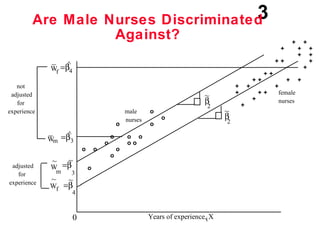
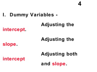
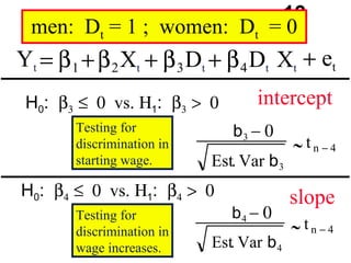
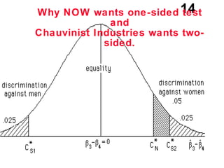
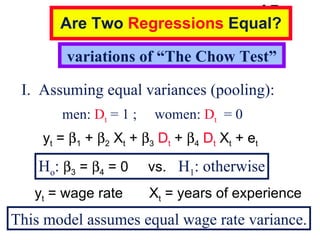
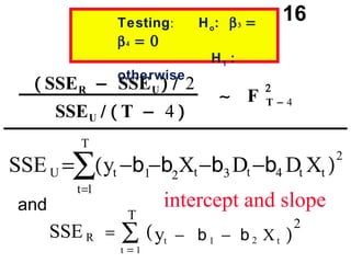
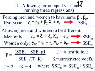
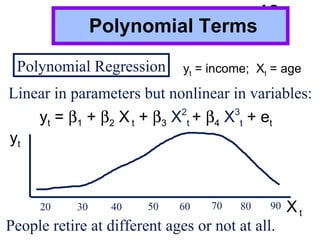
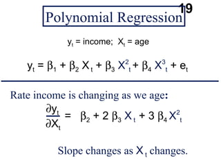
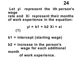
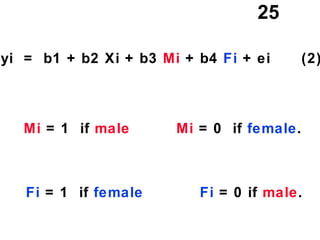
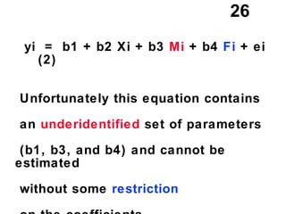
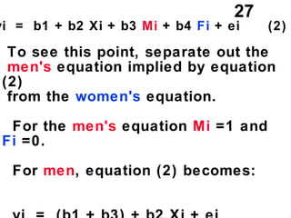
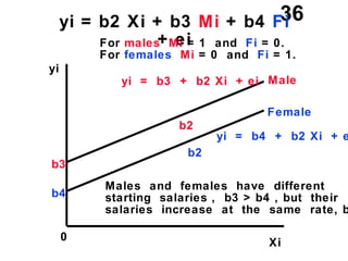
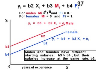
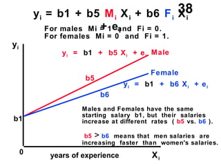
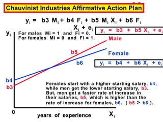
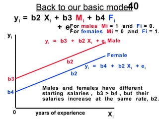
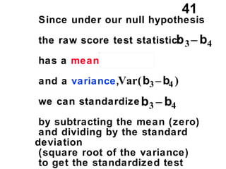
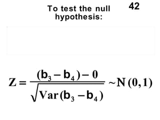
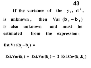
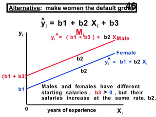
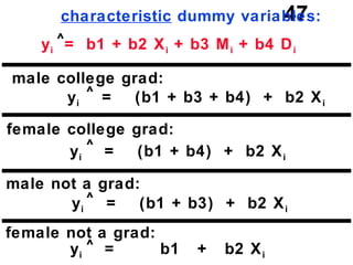
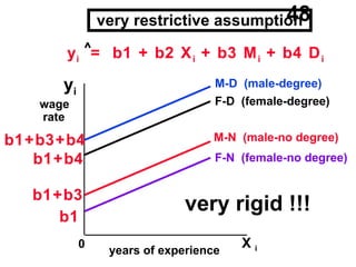

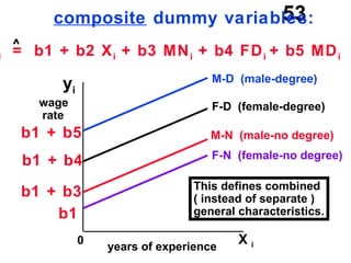
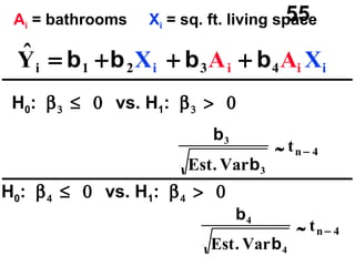
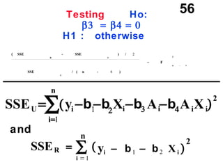
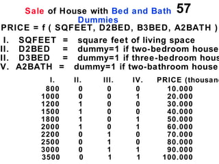
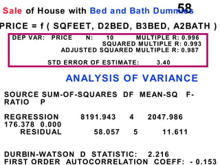
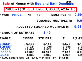
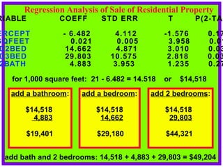

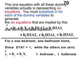
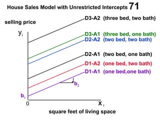
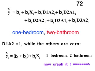
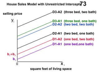


The document discusses the use of dummy variables in wage discrimination models, focusing on how different adjustments for male and female wage rates can reveal discrimination in starting wages and wage increases. It outlines methods like the Chow test for assessing whether the regressions for men and women are equal and addresses issues of underidentification in regression models. Various models are presented to analyze the impacts of experience and gender on wage rates, demonstrating how to test for differences in intercepts and slopes.


![[001081].pptx[001081].pptx[001081].pptx[001081].pptx[001081].pptx[001081].pptx](https://cdn.slidesharecdn.com/ss_thumbnails/001081-241031195449-7a555459-thumbnail.jpg?width=640&height=640&fit=bounds)