Assessment of Fatigue Failure in FPSO Mooring Systems

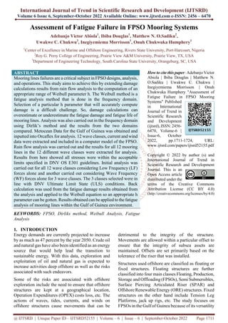
International Journal of Trend in Scientific Research and Development (IJTSRD)
Volume 6 Issue 6, September-October 2022 Available Online: www.ijtsrd.com e-ISSN: 2456 – 6470
@ IJTSRD | Unique Paper ID – IJTSRD52155 | Volume – 6 | Issue – 6 | September-October 2022 Page 1711
Assessment of Fatigue Failure in FPSO Mooring Systems
Adebanjo Victor Abiola1
, Ibiba Douglas1
, Matthew N. O.Sadiku2
,
Uwakwe C. Chukwu3
, Inegiyemiema Morrisson1
, Onuh Chukwuka Humphery1
1
Center of Excellence in Marine and Offshore Engineering, Rivers State University, Port-Harcourt, Nigeria
2
Roy G. Perry College of Engineering, Prairie View A&M University, Prairie View, TX, USA
3
Department of Engineering Technology, South Carolina State University, Orangeburg, SC, USA
ABSTRACT
Mooring lines failures are a critical subject in FPSO designs, analysis,
and operations. This study aims to achieve this by extending damage
calculations results from rain flow analysis to the computation of an
appropriate range of Weibull parameter h. The Weibull method is a
fatigue analysis method that is done in the frequency domain.
Selection of a particular h parameter that will accurately compute
damage is a difficult challenge. So, damage calculations can
overestimate or underestimate the fatigue damage and fatigue life of
mooring lines. Analysis was also carried out in the frequency domain
using Dirlik’s method and the results from the two domains
compared. Metocean Data for the Gulf of Guinea was obtained and
inputted into Orcaflex for analysis. 12 wave classes, current and wind
data were extracted and included in a computer model of the FPSO.
Rain flow analysis was carried out and the results for all 12 mooring
lines in the 12 different wave classes were extracted for analysis.
Results from here showed all stresses were within the acceptable
limits specified in DNV OS E301 guidelines. Initial analysis was
carried out for all 12 wave classes considering Low Frequency (LF)
forces alone and another carried out considering Wave Frequency
(WF) forces alone for 3 wave classes. The 3 classes selected were in
line with DNV Ultimate Limit State (ULS) conditions. Back
calculation was used from the fatigue damage results obtained from
the analysis and applied to the Weibull equation so an appropriate h
parameter can be gotten. Results obtained can be applied to the fatigue
analysis of mooring lines within the Gulf of Guinea environment.
KEYWORDS: FPSO, Dirliks method, Weibull Analysis, Fatigue
Analysis
How to cite this paper: Adebanjo Victor
Abiola | Ibiba Douglas | Matthew N.
O.Sadiku | Uwakwe C. Chukwu |
Inegiyemiema Morrisson | Onuh
Chukwuka Humphery "Assessment of
Fatigue Failure in FPSO Mooring
Systems" Published
in International
Journal of Trend in
Scientific Research
and Development
(ijtsrd), ISSN: 2456-
6470, Volume-6 |
Issue-6, October
2022, pp.1711-1724, URL:
www.ijtsrd.com/papers/ijtsrd52155.pdf
Copyright © 2022 by author (s) and
International Journal of Trend in
Scientific Research and Development
Journal. This is an
Open Access article
distributed under the
terms of the Creative Commons
Attribution License (CC BY 4.0)
(http://creativecommons.org/licenses/by/4.0)
1. INTRODUCTION
Energy demands are currently projected to increase
by as much as 47 percent by the year 2050. Crude oil
and natural gas have also been identified as an energy
source that would help lead the transition to
sustainable energy. With this data, exploration and
exploitation of oil and natural gas is expected to
increase activities deep offshore as well as the risks
associated with such endeavors.
Some of the risks are associated with offshore
exploration include the need to ensure that offshore
structures are kept at a geographical location,
Operation Expenditures (OPEX) costs loss, etc. The
actions of waves, tides, currents, and winds on
offshore structures cause movements that can be
detrimental to the integrity of the structure.
Movements are allowed within a particular offset to
ensure that the integrity of subsea assets are
maintained. Offsets are set primarily based on the
tolerance of the riser that was installed.
Structures used offshore are classified as floating or
fixed structures. Floating structures are further
classified into four main classes Floating, Production,
Storage and Offloading (FPSOs), Semi Submersibles,
Surface Piercing Articulated Riser (SPAR) and
Offshore Renewable Energy (ORE) structures. Fixed
structures on the other hand include Tension Leg
Platforms, jack up rigs, etc. The study focuses on
FPSOs in the Gulf of Guinea because of its versatility
IJTSRD52155

International Journal of Trend in Scientific Research and Development @ www.ijtsrd.com eISSN: 2456-6470
and reduced Capital Expenditure (CAPEX) in
relations to other structures designed to operate in
deep water conditions. Also being considered is the
need to ensure that there is a dependable framework
for fatigue analysis in the Gulf of Guinea. Mooring
systems are of two types. They include the temporary
and permanent mooring system. The temporary type
finds major application in pipe laying vessels, lift
vessels, etc. while the latter has more stringent rules
since they find application in offshore structures
designed to be positioned in a location for long.
Various considerations are infused during the design
of the structures. Chief amongst these considerations
is the load imposed by the environment. Major
contributors include wave, current and wind.
Continuous applications of these loads induce various
stresses which when continuously applied induces
fatigue stresses that are bound to cause failures if not
effectively considered during the design stage of the
mooring lines. According to Ma et al. (2013) many of
these failures have been reported in various offshore
sites across the world. Causes of failures vary from
improper design, poor quality of mooring line
components and poorly trained operators.
With operations regarding exploration moving deep
offshore, the industry needs to improve available
methods and adequately scrutinize their accuracies on
the field. Mooring lines comprises of a top chain,
bottom chain, and a rope/ polyester wire. The
configurations become trickier as operational depth
increases. This is because using a chain all through
would be counterproductive when weight increments
in relation to the vessel’s self-weight is considered.
Major mooring accidents have occurred, and the
potential impacts become reinforced with the
ambitious move towards deep exploration.
Mooring systems are organized in three ways which
include: taut mooring; catenary mooring and catenary
mooring with buoyancy elements. Some of the
features of a mooring line are:
1. Taut mooring made up of chain-synthetic fiber
ropes/polyester-chain
2. Catenary mooring made up of chain-steel rope-
chain
3. Catenary mooring with buoyancy elements made
up of chain-steel wire rope-buoy-steel wire rope-
chain.
With increasing leap and movement towards deep
water exploration catenary systems are more
unpopular and inapplicable due to the increasing
weight. Taut leg mooring was developed as a solution
to this challenge. In the taut system the seabed is
approached horizontally at an angle. The arrangement
ensures the ability of the system to resist both
horizontal and vertical forces. Catenary systems
address horizontal forces alone which is contributed
by the weight of the mooring lines.
Larsen (2014) gave a vivid description as shown in
the figure below: 1 represents taut mooring,2
represents catenary system and 3 represents catenary
mooring with buoyancy elements. Some of the
features incorporated into various mooring systems
include anchor, chain synthetic fiber ropes, buoys,
clump weights etc.
For chains, their configurations may be stud less or
stud link. For chains that must be rearranged several
times during their deployment. The weights of the
chains are heavy and more likely to be subjected to a
great deal of fatigue damage when they are related to
others. Larsen (2014) did a comparative study of the
properties of the materials used in mooring lines. It is
shown in the table 1 below
Table 1: Properties of some mooring lines
Material
Diameter
(mm)
Weight in
air (kg/m)
Weight in
water (kg/m)
Typical Axial
Stiffness*10^-5 (KN)
Stud R4 chain 102 230 200 7
Spiral Strand Steel 108 57 48 9
Polyester 175 23 5.9 1.0-4.5
For steel wire ropes several spiral strands which may be covered or uncovered by a plastic sheet are commonly
found on most. They are not as heavy as chains and are known to have good fatigue properties consequently
making them less of a concern. In shallow waters, they are known to have small fatigue capacity at shallow
depths.
For synthetic ropes polyester is one of the most used materials but other high-tech fibers are also deployed.
These ropes are known to have less weight but are highly elastic. Ascertaining Fatigue Limit States (FLS)
require intricate analysis that are known to be time consuming.
Getting a good grip of the safety requirements of offshore structures makes fatigue an important subject. Its
classification is based majorly on how they occur and may vary from mechanical, creep, thermo-mechanical,

corrosion and fretting fatigue. Berge (2006) emphasized that the constantlyoccurring loads which are lesser than
the material yield strength accumulates and lead to material failure.
Fatigue cracks are known to spread and lead to failures in three different modes which are tension, shear and
torsion. Asides the aforementioned, In-plane Bending (IPB) and Out of Plane Bending (OPB) is a major
contributor to fatigue failure in mooring lines. Yooil et al (2018) carried out an investigation on this concept by
combining both hydrodynamic and stress analysis methods. Hydrodynamic analysis was done using the
decoupled analysis method and the stress analysis method involved the use of non-linear finite element analysis
method.
Rampi et al (2016) employed a multi-axial approach by carrying out a fatigue test with a full-scale chain model.
A Finite Element Method (FEM) analysis was also carried out before result comparison. Theyrecommended the
use of the multi axial fatigue criterion as opposed to the uniaxial maximum principal stress criterion.
Kim and Kim (2017) evaluated parametrically the stiffness and stress concentration factor which is introduced
by IPB and OPB elements. A sensitivity analysis was also conducted on the result to ascertain the significance of
the impacts of the numerical friction model.
Fatigue computations are done using a Time Domain (time domain) or Frequency Domain (FD) analysis. Wave
loading is known to make results from the results below very uncertain Uncertainty here is made pronounced by
the drag forces though wave modelling of waves occurring near the sea surface and current is weighty.
Probabilistic/stochastic Frequency Domain (FD) analysis makes it possible to evaluate damage due to fatigue
using two approaches that involves application of stress spectrum that exist in a cross section of the object being
subjected to test. The methods include:
 Gaussian methods which are seen as a narrow-banded process that involves the application of Rayleigh
distribution computation approach on ranges of peaks and stress.
 Fast Fourier Transform (FFT) application on stress spectrum to generate a stress history that results in a
broad branded Gaussian process. Stress history generated is used to compute fatigue damage by cycle and
range counting. From this process, the total fatigue damage results are obtained.
 Time domain (TD) analysis is also approached in two ways, and they include:
 Carrying out a rain flow counting analysis which is known to produce results in record time as it uses not so
much computation resources.
 Probability distribution selection that is used to estimate parameters based on load historywhich can be used
to calculate fatigue damage by integrating the Probability Density Function (PDF) and the S-N curve.
TD and FD methods can be further broken down into various methods. FD methods include Simple Summation
(SS) approach, Combined spectrum method, Dual Narrow Band (DNB). For TD, methods used include Weibull
and the Rainfall Analysis Method. Weibull analysis is based on the closed fatigue life equation and an
assumption that a hypothetical structure has stress cycles that are stochastic and have a Probability Distribution
Function (PDF). Asides the aforementioned, spectral (also frequency) methods such as the Dirlirk’s approach are
used. Propounded in 1985, it aims to estimate the Probability Density Function (PDF) of specific stresses from
Power Spectral Density (PSD) obtained from the frequency response of a system. Moments are calculated and
used to calculate the damage of a system. Pankaj (2017) applied Dirlik’s method to the computation of fatigue
stresses in tubular structures, verifying the accuracy of the method in the process. It is known to be more
accurate when compared to the Rainflow counting method.
2. METHODOLOGY
The field used for the study is located about 120 km off the coast of the South-Eastern region of Niger Delta
with coordinates 4.5569°N and 4.6169°E. Metocean conditions in this region are mild and are a function of its
position relative to the Inter-Tropical Convergence Zone (ITCZ). Conditions in this region vary from periods
with light winds, afternoon rain showers, periods of short-lived intense rainfall, and relatively low wave heights.
Metocean data for wind, waves and currents were used for the analysis.
Data used for this thesis was obtained from the Marine Copernicus data repository for metocean data and the
downloaded file opened using MATLAB. Geographical coordinates were used to extract the data for the
analysis. The wave classes used for the study is shown in the table below.

Table 2: Wave classes for analysis
S/N Direction Hs(m) Tz(s)
1 180 3.42 12.72
2 230 3.42 17.60
3 230 2.77 19.47
4 230 2.77 9.70
5 190 3.19 10.60
6 190 3.55 7.30
7 166 3.85 12.00
8 220 4.09 12.00
9 220 2.32 15.60
10 215 2.07 15.90
11 2.30 1.76 14.00
12 185 2.90 16.90
The Guinean current flows along the coast of West Africa in a direction between 2- and 5-degree North.
(Djakoure et al., 2017) A surface speed of 2.13 m/s and a seabed speed of 0.19 m/s was used for the analysis.
Orcaflex computes current profiles using the interpolated or the power law method. The power law method was
used.
2.1. Vessel Description
The FPSO used a case study is installed off the coast of Nigeria and operates in waters that are about 1000m
deep. It is spread moored with 12 mooring lines and has a heading of 180 degree in Southwestern direction to
reduce the effect of waves on vessel stability. Configuration of mooring lines include a studless top chain,
multistrand wire rope and a studless bottom chain. About 1 mile from the FPSO is a Single Point Mooring
(SPM) buoy for the offtake of crude produced from the field. A summary of the mooring chain lengths and
vessel properties are shown in the tables 3.2 and 3.3 below.
Table 3: Vessel Parameters (Chanhoe et al., 2016)
Parameters Value
Length (m) 305.1
Breadth (m) 58
Depth (m) 21.2
Summer DWT (Tonnes) 350,000 tonnes
Table 4: Table of mooring line segments length
S/N Mooring Chain Section Diameter (m) Section Length(m)
1 Portside line 1-6
Top Chain 0.178 101.20
Wire Rope 0.098 1103.00
Bottom Chain 0.178 669.60
2 Starboard Line 1-3
Top Chain 0.178 96.20
Wire Rope 0.098 1133.60
3 Starboard 4-6
Top Chain 0.178 96.00
Wire Rope 0.098 1101.50
2.2. Simulation in Orcaflex
Dynamic analysis builds on the positional outcome obtained from the static analysis of a model. It simulates the
motion of the model over an appropriate period taking into cognizance the metocean data inputted, the Response
Amplitude Operator (RAO), vessel headings, draught and other factors.
A build-up stage precedes dynamic simulation during which motions that encompass low frequency (LF) and
Wave Frequency (WF) are slowly revved up from zero to their full size. Currents which are a component of LF
motions can be left out of the whole ramping up operations to cut down on transients generated by the switch
from static to dynamic analysis.

The unit of time in the software is seconds and wave time origins can be set when inputting wave data. When set
to zero (as used in the simulations) wave effects application starts at global time 0 at the end of the revving up
stage. Other entries asides 0 which consequently time shifts the wave application time. When several waves are
applied, time origins can be spread apart so simulation stages can be spread out.
Model in Orcaflex includes 12 mooring lines, FPSO and a SPM buoy. Risers, water injector pipes, gas export
lines, etc. have all been removed to optimize model and reduce simulation runtime. Model used is shown figure
1 below.
Figure 1: FPSO Model in Orcaflex
As part of efforts to Quality Check (QC) the model, attention was given to the grade/type, diameters, and
breaking load values of the mooring line components. This was specified and checked using the line type wizard
and its data repository for the breaking load. Identifying and making adequate checks in this area also helps
select appropriate values (m and k) for the TN curve used for rainflow analysis after loading the simulation files.
DNV recommends the following values. Breaking strength is also added for emphasis.
Table 5: DNV recommended values used for fatigue analysis
Chain/Rope Type m k Breaking Strength(KN)
Stud less Chain (R4) 3 316 25480
Spiral Strand Wire Rope 4 1000 8000
Low and wave frequency components were also accounted for according to DNV guidelines. The software
allows the user to account for these components in simulation runs or both. When running a model using both
options a threshold frequency must be set. One thing to be observed was to select the right effects that were
applicable to wave or low frequency responses. The possible options include applied loads, wave loads, wave
drift load, wave drift damping, sum frequency load, added mass damping, maneuvering load, other damping,
current load and wind load. Setting the primary motion to either low, wave or both automatically selects the
appropriate primary effects to be used for the runs when all effects are included regardless of anyoption selected
that is not applicable to the primary motion selected. Results were loaded on conclusion of simulation to obtain
stress, tension, zero crossing period, etc. from the simulation files for use in Weibull computation and analysis.
2.3. Weibull Analysis Case Study
This section assesses how computations are carried out using Wave 1 as an instance on how computations were
carried out. Wave 1 simulation files for LF and WF primary motions were used to extract important data used
for computations for mooring line P1. It is important to note that all forces and stresses induced in line P1 were
checked to ensure that it is safely within the breaking loads of the line components. The extreme statistics option
in the software helped predict the maximum tension in line P1 during a 3-hour storm. Prediction results showed
a 95 percent confidence limits and showed the effective tension is 9664.68KN. The table below shows other
values extracted using the linked statistics and result summary options in the software.

Table 6: Parameters List Obtained from dynamic simulation results in Orcaflex
S/N Variable Name Value
1 Standard deviation of Low frequency stress component ( 12934.9415 KN
2 Standard deviation of Wave frequency stress component ( 11027.2651KN
3 Mean up Crossing Period Tz (s) for the stress component in LF motions 0.1863 sec
4 Mean up Crossing Period Tz (s) for the stress component in WF motions 0.1914 sec
5 Most probable maximum tension ( ) 11,9583 KPa
6 Mean stress ( 55350.479 KPa
The Weibull Expression used for the calculations is shown below.
3.6
Where, is the gamma function
is the maximum stress range of stress cycles
is the total number of stress cycles
m is the negative inverse slope of the SN curve
is the antilog of the intercept of the Log N axis of the SN-curve
h is the Weibull parameter
D is the damage per year
To compute the normalized variance λ of LF and WF motions, the expressions below are used:
(1)
(2)
For
For
Since frequency is the inverse of period, the zero up crossing frequencies for LF and WF motions is calculated
below.
For ,

To calculate the up-crossing rate through the mean value of the stress spectrum for the combined process, the
expression below is used.
(3)
Where is the bandwidth parameter taken as 0.1 according to DNV guidelines.
To compute the total number of stress cycles , .
(4)
Where represents the total time in seconds the wave phenomenon lasts for 1year. An assumption is
made here that the wave occurs once a day for 12.72 seconds.
Maximum stress range is computed using the formula below.
(5)
The damage D is computed using the values obtained from the rainflow fatigue analysis carried out in the
software. The wire rope section here is used for computation. The values gotten from the simulation is shown in
the table 3.6 below.
Table 7: Damage parameters obtained from software
Section length Total Damage Per day Damage Per year
1103m 6.3286E-09 2.3099e-06
DNVGL-OS-E301 recommends a value for m and as shown in the table below. This also applies to different
line components.
Table 8: DNV recommended values for SN curve
Line Component m
Studless chain 3.0
Spiral Rope 4.8
On substitution of all parameters into the Weibull equation, the expression can be written as
A MATLAB code is used to solve this. From results generated from the m file run, the values of h varies from
0.8869 to 0.900 suggesting that the answers are well within acceptable range of h values. The method shown
above is then repeated for three wave classes and all mooring lines.
2.4. Fatigue Damage in Frequency Domain (Dirlik Method)
To compute fatigue in frequency domain a Power Spectral Density (PSD) diagram of the load is an important
aspect. It gives information about the magnitude of a a normalized power in frequency domain. Fourier
transform (f(w)) is obtained from a time series using the equations below:

(6)
(7)
Where is the frequency in Hz and t is the total time.
The unit of PSD is unit2
/Hz and is obtained from MATLAB using the pwelch command. The stress time history
obtained from dynamic simulation carried out in Orcaflex. Data extracted does not include the buildup stage in
Orcaflex since the stage 1 simulation is the most important in this case. Tension cycles vary depending on the
node being studied. In other to deal with this, data from nodes at regular intervals are extracted and their
corresponding PSDs plotted in MATLAB for use in Dirlik’s formula.
PSDs obtained from the tension cycles also had their corresponding data plots extracted and put in a excel file.
Entries run as high as 16386 for the x and y axes respectively. From these values the moments of the curve are
computed and applied for use based on Dirlik’s method. The expressions used are shown in subsequent sections.
To calculate moments , and , the expression below is used
(8)
Where is the frequency
is the output PSD in terms of stress amplitude
The expression above is important in computing the number of cycles N(S). Expression for computation is
shown in the expression below.
(9)
Where T is the total time considered for fatigue damage computation, E(P) is the expected number of peaks and
p(S) is the probability of stress range S computed by using the expression below.
(10)
(11)
The constants used in the expression above is computed using the expressions below.
(12)
(13)
(14)
(15)
(16)
(17)
(18)
(19)
In the expressions above is the mean frequency, Z refers to the normalized stress range, is the irregularity
factor and other parameters refer to constants.
Once all computations required are executed, a plot of various stress ranges (S) and the Probability Density
Function (PDF) is carried out. The area under the curve gives the fatigue damage, D. Calculations carried out
were on mooring line S3 alone and were executed in MATLAB.

3. RESULTS AND DISCUSSION
The Figure 2 below shows the total damage on mooring lines located on the starboard side of the vessel. It
reveals a lot of information about which mooring line on the FPSO is more likely to experience a higher amount
of damage. Careful observation shows that S4 is more likely to experience a higher amount of damage with S5
and S6 having a similar profile. It is important to note that S4 to S6 are located to the aft of the FPSO. S1 to S3
from the charts is observed to have a lower damage profile on all line segments. Candidates for regular checks
would be the S4 to S6. It is important to note that low damage profile doesn’t guarantee reliability. In-Plane
Bending (IPB) and Out of Plane Bending (OPB) are also known to cause failures in rightly designed chains as a
lot of normal bending stresses are introduced.
Figure 2: Total Damage across Mooring Line Lengths (S1-6)
Figure 3: Total Damage across Mooring Line Lengths (P1-6)
The damage profile of P1 to P6 as shown in figure 2 above start at higher levels when compared to that of S
series. This can be attributed largely to the FPSO orientation and metocean conditions. The impacts of forces
induced by LF motions can be attributed to this as well. P5 and P4 have the highest profiles on all sections of the
mooring lines and look like damage in the bottom chains are a bit erratic. All mooring lines in the analysis have
sections where the damage readings are at 0. Similarities in the damage profile structure is observed because all
lines have similar mechanical properties and structural arrangements as seen in the table of the mooring lines
segment.
The fatigue life curves of the portside and starboard sides obtained from Orcaflex simulation results is shown in
figure 4 and 5 below. Amongst the P series, P2 and P3 have the highest fatigue life owing to their very low

damage profile as seen in the preceding figures. P4 and P5 have the lowest fatigue life in all sections. The S
series lines have higher fatigue lives and consequently more likely to last longer than the P series lines.
Figure 4: Fatigue Life across all Mooring Line Lengths (P1-6)
Figure 5 Fatigue Life across all Mooring Line Lengths (S1-6)
3.2. Frequency Domain Fatigue Analysis
This section addresses the fatigue damage of mooring line S3 at Ends A and B in frequency domain as well as
key results obtained from dynamic simulation in Orcaflex. Results obtained from the simulations were used as
inputs for Dirlik formula applications and Power Spectral Density (PSD) computations.
Figure 6 below shows the time history of tensions at ends A and B of the mooring line. End A is the point of
attachment of the mooring line to the vessel while End B refers to the attachment to the suction pile at
touchdown. Simulation history results extracted excluded the build-up stage of the run so extraction starts from
time 0 seconds. Time interval of the tensions 0.05 is 0.05 seconds over a duration of 5400 seconds. Total number
of data points extracted for each of the plots below is 108,000 points. The spectra obtained after plotting are
narrow banded at some point. Time history of End B can be said to be narrow banded for all time durations.
However End A is narrow banded from 0 to around 2743 seconds after which the tension range becomes

magnified. This turns the spectrum to a bimodal type. The maximum tension developed in the mooring line at
End A is 9362 KN while the least tension developed at this end is 19.66KN. At End B the results are way lesser
than End A. The maximum effective tension developed here is 1399KN and the least is 1136 KN. The stress
time history is also similar to the tension time history.
500 1000 1500 2000 2500 3000 3500 4000 4500 5000 5500
Time(s)
1000
2000
3000
4000
5000
6000
7000
8000
9000
Effective Tension Time History at End A
Figure 6: Tension Time History of Mooring Line at Ends A and B
Tension cycles can be extracted across all nodes on the mooring lines so closer examination of the variation of
tension across all nodes can be closely assessed to identify areas of high tension and for more detailed damage
considerations. The stress derivative of the tension cycle above was used as a basis for the computation of the
Power Spectral Density (PSD) for ends A and B shown in the figures below.
Figure 7: Power Spectral Density (PSD) for End B

Figure 8: Power Spectral Density (PSD) for End A
Power spectral Density (PSD) is an important stage in the computation of fatigue damage in the frequency
domain. It shows the impacts or strengths of the tension signals at various frequencies. The peak in the figure
indicates areas of interest whose frequencies have been normalized. The region under the PSD curves represents
the power of the spectrum.
On completion of computation, using the Dirlik’s method the results of the damage done at an interval of 300 is
shown in Table 4.2 below.
Table 9: Table of Damage obtained using Dirlik’s Method
Arc Length (m) Damage
0 7.80E-07
320 1.24E-08
640 1.24E-08
960 7.27E-09
1280 1.01E-07
1600 5.78E-08
1920 5.31E-08
A plot of the results is shown in Figure 9 below. The figure also helps compares the damage results obtained
from both methods used in the thesis. Both methods show that the results have similar trajectories and profiles
along over 50 percent of the mooring line arc lengths.
Figure 9: Results Comparison of Dirlik and Rainflow analysis Results.

3.3. Weibull Analysis Results
Results from this session aims to identify and constrict the range of values that will be recommended. Data used
for the plots is shown below for two wave classes. It represents results for the wire rope section. Wave 3 is
selected to represent the ULS state the FPSO is being designed to operate in.
Figure 10: Average h parameters obtained from analysis.
Analysis of the results in the previous session helps streamline the possible values of the weibull parameter
down to a range between 0.8 and 1.2 marked by the thick lines in the figure.
4. CONCLUSION
The research was carried out to analyze fatigue life of
mooring lines and come up with a more streamlined
Weibull h parameter for analysis in the Gulf of
Guinea. The results of the thesis helped streamline the
already existing range of h parameters down to a
range of 0.4 (0.8 to 1.2) from 1.0(0.5 to 1.5) specified
by Weibull in his research. 12 Wave classes were
analyzed using LF forces considerations that were
specified in the software. For Weibull analysis,
simulations were carried out considering WF and LF
motions (combined) as well in line with DNV
regulations. Some of the inbuilt options in the
software that made this possible include applied load,
wave load, wave drift load, wave drift damping,
added mass damping etc.
The results from Rain flow analysis in orcaflex also
showed that all maximum and minimum stresses in
all the mooring lines were within the limits of the
breaking strengths specified according to DNV OS
E301guidelines. Dirlik’s method application also
showed the fatigue damage performance over the
periods of exposure was very safe. Fatigue life
computed showed the mooring lines will be able to
last for more than 500 years. However, the analysis
was carried out without risers and offtake buoy. As a
result, further analysis must be done to access their
impacts.
REFERENCES
[1] BERGE. (2006). Fatigue and Fracture Design
of Marine Structures.
[2] Chanhoe Kang, C. L. -H. -T. (2016). Fatigue
Analysis of Spread Mooring Line. International
Journal of Geological and Environmental
Engineering, 504-510.
[3] Curtis E. Larsen, T. I. (2014). A review of
spectral methods for variable amplitude fatigue
prediction and new results. 3rd International
Conference on Material and Component
Performance under Variable Amplitude
Loading, VAL2015 (pp. 243-250). Elsevier.
[4] K. T. Ma, A. D. (2013). A historical review on
integrity issues of permanent mooring system .
Offshore Technology Conference. Houston.
[5] Kim Y., K. M. (2017). Nonlinear Finite
Element Analysis for Mooring Chain
Considering OPB/IPB. Journal of Ocean
Engineering Technology, 299-307.
[6] Pankaj Dheer, D. I. (2017). Fatigue assessment
of offshore tubular Structures Using Dirlik's
Method to Establish the Procedure. Delft
University of Technology.
[7] Rampi L., B. A. (2016). Chain Out of Plain
Bending (OPB) Fatigue Joint Industry Project

(JIP) FEA Results and Multiaxiality Study
Results. 35th International Conference on
Ocean, Offshore and Arctic Engineering .
[8] S. DJAKOURÉ, P. P. (2017). Respective Roles
of the Guinea Current and Local Winds on the
CoastalUpwelling in the Northern Gulf of
Guinea. Journal of Physical Oceanography,
1367-1387.
[9] Yooil Kim, M. -S. K. -J. (2018). Fatigue
analysis on the mooring chain of a spread
moored FPSO considering the OPB and IPB.
International Journal of Naval Architecture
and Ocean Engineering, 178-201.

Assessment of Fatigue Failure in FPSO Mooring Systems

Recommended

Recommended

More Related Content

Similar to Assessment of Fatigue Failure in FPSO Mooring Systems

Similar to Assessment of Fatigue Failure in FPSO Mooring Systems (20)

More from ijtsrd

More from ijtsrd (20)

Recently uploaded

Recently uploaded (20)

Assessment of Fatigue Failure in FPSO Mooring Systems