
![Interactive, scalable, reproducible data analysis
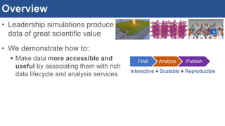
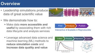
Data science and learning applications require:
- Interactivity
- Scalability
- You can’t run this on a desktop
- Reproducibility
- Publish code and documentation
Our solution: JupyterHub + Parsl
Interactive computing environment
Notebooks for publication
Can run on dedicated hardware
PARSL
parsl-project.orgjupyter.org
• Python-based parallel scripting library
• Tasks exposed as functions (Python or bash)
• Python code used to glue functions together
• Leverages Globus for auth and data movement
@App('python', dfk)
def compute_features(chunk):
for f in featurizers:
chunk = f.featurize_dataframe(chunk, 'atoms')
return chunk
chunks = [compute_features(chunk)
for chunk in np.array_split(data, chunks)]](https://image.slidesharecdn.com/20171107-sc-final-171116201216/85/Going-Smart-and-Deep-on-Materials-at-ALCF-38-320.jpg)

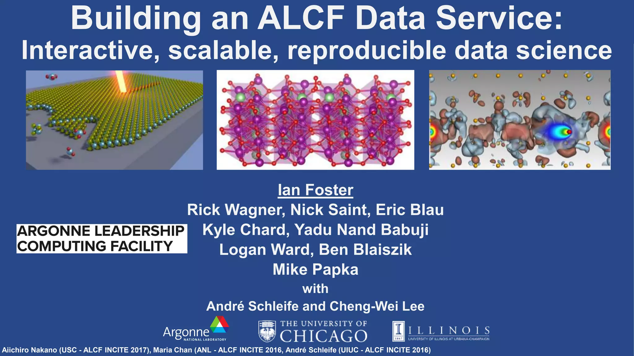
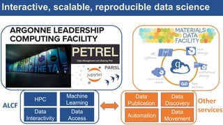
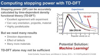
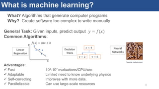
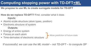
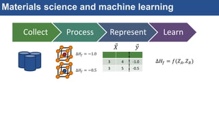
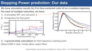
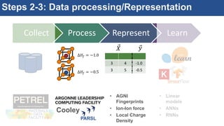
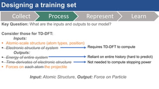
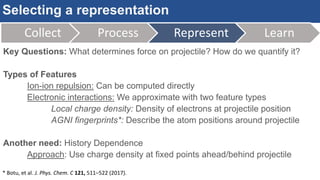
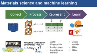
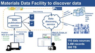
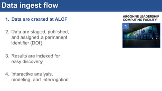
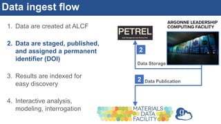
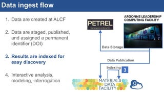
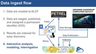
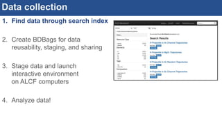
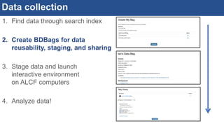
The document discusses the development of an interactive and scalable data service for advanced materials science at the Argonne Leadership Computing Facility (ALCF), emphasizing the integration of advanced data analytics and machine learning to enhance simulation capabilities. It outlines methodologies for making data more accessible, automating processes, and creating reusable data objects to promote reproducibility in scientific research. Additionally, it highlights the application of time-dependent density functional theory and machine learning in predicting stopping power in materials, illustrating the significance of this service in improving computational efficiency and scientific discovery.