Modeling firm clay compressive strength

http://www.iaeme.com/IJARET/index.asp 73 editor@iaeme.com
International Journal of Advanced Research in Engineering and Technology
(IJARET)
Volume 6, Issue 12, Dec 2015, pp. 73-85, Article ID: IJARET_06_12_008
Available online at
http://www.iaeme.com/IJARET/issues.asp?JType=IJARET&VType=6&IType=12
ISSN Print: 0976-6480 and ISSN Online: 0976-6499
© IAEME Publication
___________________________________________________________________________
MODELING AND SIMULATION OF
COMPRESSION STRENGTH FOR FIRM
CLAY IN SWAMPY AREA OF AHOADA
EAST
Eluozo. S. N
Subaka Nigeria Limited Port Harcourt Rivers State of Nigeria
Director and Principal Consultant Civil and Environmental Engineering,
Research and Development
Ode T
Department of Civil Engineering, faculty of Engineering
Rivers State University of Science and Technology Port Harcourt
ABSTRACT
The behaviuor of firm clay should be observed in design and construction
of any projects, the deposition of firm clay were monitored to determined its
compressive strength in swampy area of Ahoada east, these type of formation
are observed to be influenced by other environmental changes, it definitely
generate vertical and horizontal shrinkage on drying and expansion of wetting
during seasonal variation, the tendency of seasonal volume changes under
vegetation covers that extend to about one metre or more, the study of firm has
been observed to be influenced by seasonal variation, these conditions are
most influences observed in firm clay, the study of predicting compressive
strength for firm clay were imperative to monitor the rate of increment in
various depth at the study environment, several determination of compression
index has been produced through experimental data and empirical solutions,
these concept has not been thorough applied to determined its effective in
predicting compression strength on its index for firm clay, These applied
concepts has generated theoretical valued from simulation process, these
results were subjected to comparative test, both parameters developed
faviourable fits validating the generated model for firm clay
Key words: Modeling and Simulation, Compressive Strength, and Firm Clay

Eluozo. S. N and Ode T
Cite this Article: Eluozo. S. N and Ode T, Modeling and Simulation of
Compression Strength for Firm Clay in Swampy Area of Ahoada East.
International Journal of Advanced Research in Engineering and Technology,
6(12), 2015, pp. 73-85.
http://www.iaeme.com/IJARET/issues.asp?JType=IJARET&VType=6&IType=12
1. INTRODUCTION
The surface settlement resulting from consolidation settlement may range from a few
centimeters up to several meters, depending on the thickness of the clay deposit, its
previous loading history and the magnitude of the increased stress caused by the new
embankment load. In contrast to primary consolidation, secondary consolidation is
long-term form of settlement that occurs under a constant vertical effective stress (i.e.,
the vertical effective stress is not changing with time). In secondary consolidation, the
excess pore pressure dissipation associated with primary consolidation has essentially
dissipated, thus secondary consolidation is a decrease in void ratio change that occurs
after primary consolidation and progresses under a constant vertical effective stress.
Secondary consolidation is characterized by a continuing decrease in void ratio
resulting from rearrangement of the soil fabric with time Steven and Hap 2004.
Many experimental studies have shown that natural fine grained soils are
anisotropic and that anisotropy is related to the K0 stress conditions associated with
the process of sedimentation and the plastic straining during consolidation. Initial and
induced anisotropy of natural soils have been also investigated according to the shape
and the inclination of yield curves plotted in p’:q plan (Mitchell and Wong, 1973,
Tavenas and Leroueil, 1979, Graham et al., 1983, Leroueil and Vaughan, 1990,
Wheeler et al., 2003).
The mechanical response of natural clays strongly depends on changes in
microstructure; in particular when the initial preferential orientation is modified by
further loading paths having a different orientation with respect to the initial principal
stresses (Hicher et al., 2000). They stressed that the main difficulty was the
experimental determination of accurate model parameters. Various authors (Dafalias,
1986, Whittle and Kavvadas, 1994 among others) have proposed to model the initial
anisotropy by considering an inclined yield curve and a hardening law depending on
the volumetric plastic strain, with possible rotation of the yield curve (Wheeler et al.,
2003). Pietruszczak and Pande (2001) have described the inherent anisotropy within
the framework of multi-laminate model. Cudny and Vermeer (2004) have shown the
limitation of Pietruszczak and Pande’s model and they proposed a modified multi-
laminate model by considering, in addition to the strength anisotropy, the
destructuration of natural clays. Pestana and Whittle (1999) extended the model of
Whittle and Kavvadas (1994) with significant changes in the form of the bounding
surface and hardening laws to provide a unified model for sands and clays. They
checked the validity of this model in clays in Pestana et al. (2002). More recently,
Wheeler et al. (2003) have demonstrated that the use of the plastic volumetric strains
alone to consider the development and erasure of plastic anisotropy may lead to
unrealistic predictions under certain stress paths. Wheeler et al. (2003) proposed an
anisotropic elastoplastic model for soft clays by relating the change of the yield curve
inclination to volumetric and shear plastic straining. As both volumetric and shear
plastic straining are related to the stress loading path and to the stress history,

Modeling and Simulation of Compression Strength For Firm Clay In Swampy Area of
Ahoada East
2. GOVERNING EQUATION
02
2

dx
dc
dx
dc
V
dx
cd
P
p
L
I
(1)
Nomenclature
PI = Plastic Index
PL = Plastic Limit
V = Void Ratio
 = Porosity
Z = Dept
The developed system generated the equation that progress the following expressions
bellow
  02
2

dx
dc
V
dx
cd
P
P
L
I
(2)
Let




0n
n
n xaC





1
11
n
n
n xnaC
 




2
211
1
n
n
n xannC
    01
1
1
2
2
 






n
n
n
n
n
n
L
I
xnaVxann
P
P
(3)
Replace n in the 1st
term by n+2 and in the 2nd
term by n+1, so that we have;
       0112
0
1
0
2  






n
n
n
n
n
n
L
I
xanVxann
P
P
(4)
i.e.
      12 112   nn
L
I
anVann
P
P
(5)
  
  12
1 1
2


 

nn
P
P
anV
a
L
I
n
n
(6)
 
 2
1
2


 

n
P
P
aV
a
L
I
n
n
(7)

These derivations generated the developed model as it is express bellow,
(8)
Subject equation (8) to the following boundary condition
    HoCandoC  1
0
 
 x
P
P
V
L
I
aaxC

 10
  010  aaoC
i.e.
010  aa (9)
   
 x
P
P
V
L
I
L
I
a
P
P
V
xC


 1
01
!2
    Ha
P
P
V
oC
L
I


 1
1
!2


V
P
P
H
a L
I
1
(10)
Substitute (9) into equation (10)
01 aa 



V
P
P
H
a L
I
0 (11)
Hence, the particular solution of equation (8) is of the form: subject to this
generated model, we have these expressions further from t5he derived solution
considering other condition in system as it produced the final model considering every
parameters expressed bellow.
 
 x
P
P
V
L
I
L
I
L
I
V
P
P
H
V
P
P
H
xC





0

 
 














1
x
P
P
V
L
I
L
I
V
P
P
H
xC 
(12)
 
 x
P
P
V
L
I
aaxC

 10

Ahoada East
3. MATERIALS AND METHOD
Standard laboratory experiment where performed to monitor compression index of
firm clay at different formation, the soil deposition of the strata were collected in
sequences base on the structural deposition at different locations, this samples
collected at different location generated variations at different depth producing
deposition of stiff clay compression at different strata, the experimental result are
applied to be compared with the theoretical values to determined the validation of the
model.
4. RESULTS AND DISCUSSION
Results and discussion are presented in tables including graphical representation of
compression index for firm clay
Table 1 Predictive Values of firm clay compression index at Different Depth
Depth [M] Predictive of Firm Clay Cc
0.2 0.004
0.4 0.0084
0.6 0.0126
0.8 0.0168
1 0.021
1.2 0.0252
1.4 0.0294
1.6 0.0356
1.8 0.0378
2 0.042
2.2 0.0462
2.4 0.0504
2.6 0.0546
2.8 0.0588
3 0.06
Table 2 Predicted and Measured of compression index for firm clay at Different Depth
Depth [M] Predictive of Firm Clay Cc Measured Values of firm Clay Cc
0.2 0.004 0.0056
0.4 0.0084 0.0102
0.6 0.0126 0.0148
0.8 0.0168 0.0194
1 0.021 0.024
1.2 0.0252 0.0286
1.4 0.0294 0.0286
1.6 0.0356 0.0378
1.8 0.0378 0.0424
2 0.042 0.047
2.2 0.0462 0.0516
2.4 0.0504 0.0562
2.6 0.0546 0.0608
2.8 0.0588 0.0654
3 0.06 0.07

Depth [M] Predictive of Stiff Clay Cc
0.2 0.00287
0.4 0.0056
0.6 0.0084
0.8 0.011
1 0.014
1.2 0.0168
1.4 0.0196
1.6 0.0224
1.8 0.0252
2 0.0287
2.2 0.0308
2.4 0.0336
2.6 0.0364
2.8 0.0372
3 0.042
3.2 0.0448
3.4 0.0476
3.6 0.0504
3.8 0.0532
4 0.056
4.2 0.0588
4.4 0.0616
Depth [M] Predictive of firm Clay Cc Measured Values of firm Clay Cc
0.2 0.00287 0.002602
0.4 0.0056 0.005206
0.6 0.0084 0.007824
0.8 0.011 0.01043
1 0.014 0.01304
1.2 0.0168 0.0157
1.4 0.0196 0.0183
1.6 0.0224 0.0209
1.8 0.0252 0.0235
2 0.0287 0.0262
2.2 0.0308 0.0288
2.4 0.0336 0.0314
2.6 0.0364 0.0341
2.8 0.0372 0.0367
3 0.042 0.0394
3.2 0.0448 0.042
3.4 0.0476 0.0447
3.6 0.0504 0.0473
3.8 0.0532 0.0499
4 0.056 0.0526
4.2 0.0588 0.0553
4.4 0.0616 0.0579

Ahoada East
Depth [M] Predictive of firm Clay Cc
0.2 0.017
0.4 0.032
0.6 0.048
0.8 0.06
Depth [M] Predictive of firm Clay Cc Measured Values of firm clay
0.2 0.017 0.0189
0.4 0.032 0.0385
0.6 0.048 0.061
0.8 0.06 0.0843
Depth [M] Predictive of firm Clay Cc
0.2 0.0031
0.4 0.006
0.6 0.009
0.8 0.015
1 0.017
1.2 0.018
1.4 0.021
1.6 0.024
1.8 0.027
2 0.03
2.2 0.033
2.4 0.036
2.6 0.039
2.8 0.042
3 0.045
3.2 0.048
3.4 0.051
3.6 0.054
3.8 0.056
4 0.06
0.2 0.0031 0.0028
0.4 0.006 0.0056
0.6 0.009 0.0084
0.8 0.015 0.0112
1 0.017 0.014
1.2 0.018 0.0168
1.4 0.021 0.0196
1.6 0.024 0.0224
1.8 0.027 0.0252
2 0.03 0.028
2.2 0.033 0.031
2.4 0.036 0.034

2.6 0.039 0.037
2.8 0.042 0.0392
3 0.045 0.042
3.2 0.048 0.045
3.4 0.051 0.048
3.6 0.054 0.05
3.8 0.056 0.053
4 0.06 0.056
Figure 1 Predictive Values of firm clay compression index at Different Depth
Figure 2 Predicted and Measured of compression index for firm clay at Different
Depth
y = -0.0008x2 + 0.0233x - 0.001
R² = 0.9985
0
0.01
0.02
0.03
0.04
0.05
0.06
0.07
0 1 2 3 4
PredictedvaluesforFirmClay
Depth [m]
Predictive of Firm Clay Cc
Poly. (Predictive of Firm Clay
Cc)
0
0.01
0.02
0.03
0.04
0.05
0.06
0.07
0.08
0 1 2 3 4
predictivevaluesforfirmclay
Depth [M]
Predictive of Firm Clay Cc
Measured Values of firm
Clay Cc

Ahoada East
Depth
y = 4E-05x2 + 0.0138x + 0.0001
R² = 0.9994
0
0.01
0.02
0.03
0.04
0.05
0.06
0.07
0 1 2 3 4 5
Depth [M]
Predictive of Stiff Clay Cc
Poly. (Predictive of Stiff Clay
Cc)
0
0.01
0.02
0.03
0.04
0.05
0.06
0.07
0 1 2 3 4 5
predictiveandmeasuredvaluesforfirmclayon
compressionindex
Depth [M]
Predictive of firm Clay Cc
Clay Cc

Depth
y = -0.0187x2 + 0.0912x - 0.0008
R² = 0.9988
0
0.01
0.02
0.03
0.04
0.05
0.06
0.07
0 0.2 0.4 0.6 0.8 1
Depth [M]
Poly. (Predictive of firm
Clay Cc)
0
0.01
0.02
0.03
0.04
0.05
0.06
0.07
0.08
0.09
0 0.2 0.4 0.6 0.8 1
predictiveandmeasuredvaluesforfirmclayon
compressionindex
Depth [M]
clay

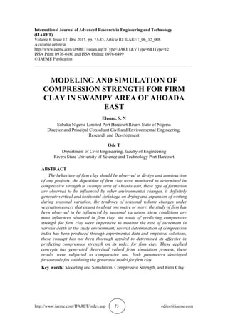
Ahoada East
Depth
The figure presented express various deposition of firm clay under compression
pressured in construction processes, figure one and two express the behaviour of firm
clay in swampy environment, the trend from the figure express gradual increment of
firm clay to the optimum level at three metres but slight fluctuation on gradual
increase of the firm soil compressibility were observed in the figure stated above,
while figure three and four maintained linear increase but at three metres sudden
slight vacillation were observed, thus linear increment of compressibility continued to
the optimum level at four metres, figure five and six expressed the progressive
condition of firm clay compressibility in linear state, but the predictive values
experiences variation compared to other deposited compression parameters expressed
y = 0.0147x + 0.0008
R² = 0.9981
0
0.01
0.02
0.03
0.04
0.05
0.06
0.07
0 1 2 3 4 5
Depth [M]
Linear (Predictive of firm
Clay Cc)
0
0.01
0.02
0.03
0.04
0.05
0.06
0.07
0 1 2 3 4 5
predictiveandmeasuredvaluesforfirm
clayoncompressionindex
Depth [M]
clay

in previous figure, the parameter predicted the compressibility at the optimum level of
less than one metres. While figure seven and eight express fluctuation between
[0.8and 1.2M] thus maintained linear compressibility from [1.3-4m] the experimental
date were compared with the predictive values from figure one to eight, both
parameters expressed best fits validating the developed model values for firm soil
compression in the study environment
5. CONCLUSION
Firm, clays are soil that compact shrink formations, definitely they suffer substantial
vertical and horizontal shrinkage through the process of drying and expansion on
wetting due to seasonal changes. These formations that experiences seasonal volume
changes under grass extend to about one metre below the surface. Most developed
nations, it is observed to extend up to 4 m or more below large trees. Definitely the
degree or volume changes, particularly in firm clay soils are determined on change
through seasonal influences variations including closeness of trees and shrubs. The
behaviour of firm can be pressured by environmental change, these implies that the
greater the seasonable variation, the greater the volume change in the formation. The
behaviour firm clay are observed in terms of foundations design and construction
subjected to it variation, these are expressed in the developed model that generated the
predictive values. The determination of compression index for firm clay are normally
generated from experimental data or empirical solutions, but for this study the
application of mathematical modeling method has not been applied in any current
literature, the developed model has definitely generated theoretical values from
simulation carried out, these were compared with experimental data, both parameters
developed faviourable fits. The figure developed various increment of firm soil
compressibility at different depths under the specification for firm soil compression
index.
REFERENCES
[1] Steven F. B; Hap S. L 2004 Estimation of Compression Properties of Clayey
Soils Salt Lake Valley, Utah Report Prepared for the Utah Department of
Transportation Research Division Civil and Environmental Engineering
Department University of Utah
[2] Cudny, M. & Vermeer, P. A. (2004). On the modelling of anisotropy and
destructuration of soft clays within the multi-laminate framework. Computers
and Geotechnics 31, No. 1, 1-22.
[3] Hicher, P. Y., Wahyudi, H. & Tessier, D. (2000). Microstructural analysis of
inherent and induced anisotropy in clay. Mechanics of Cohesive-Frictional
Materials 5, No. 5, 341-371.
[4] Leroueil, S. & Vaughan, P. R. (1990). The general and congruent effects of
structure in natural soils and weak rocks. Géotechnique 40, No. 3, 467-488.
[5] Mitchell, R. J. & Wong, K. K. (1973). The generalized failure of an Ottawa
Valley Champlain sea clay. Canadian Geotechnical Journal 10, 607-616.
[6] Graham, J., Noonan, M. L. & Lew, K. V. (1983). Yield states and stress-
strain relationships in a natural plastic clay. Canadian Geotechnical Journal
20, No. 3, 502-516.
[7] Dafalias, Y. F. (1986). An anisotropic critical state soil plasticity model.
Mechanics Research Communications 13, No. 6, 341-347

Ahoada East
[8] Pietruszczak, S. & Pande, G. N. (2001). Description of soil anisotropy based
on multilaminate framework. International Journal for Numerical and
Analytical Methods in Geomechanics 25, No. 2, 197-206.
[9] Whittle, A. J. & Kavvadas, M. J. (1994). Formulation of MIT-E3 constitutive
model for overconsolidated clays. Journal of Geotechnical Engineering-
ASCE 120, No. 1,173-198
[10] Sandhya Rani. R., Nagendra Prasad. K and Sai Krishna. T., Applicability of
Mohr-Coulomb & Drucker-Prager Models For Assessment of Undrained
Shear Behaviour of Clayey Soils. International Journal of Civil Engineering
and Technology, 5(10), 2014, pp. 104-123.
[11] Tavenas, F. & Leroueil, F. (1979). Les concepts d'état limite et d'état critique
et leurs applications pratiques à l'étude des argiles. Rev. Française de
Géotechnique 6, 27-49
[12] Wheeler, S. J., Naatanen, A., Karstunen, M. & Lojander, M. (2003). An
anisotropic elastoplastic model for soft clays. Canadian Geotechnical
Journal 40, No. 2, 403-418.
[13] S. Ramesh Kumar and Dr. K.V.Krishna Reddy, an Experimental
Investigation on Stabilization of Medium Plastic Clay Soil with Bituminous
Emulsio. International Journal of Civil Engineering and Technology, 5(1),
2014, pp. 61-65.

Modeling firm clay compressive strength

Recommended

Recommended

More Related Content

What's hot

What's hot (20)

Viewers also liked

Viewers also liked (6)

Similar to Modeling firm clay compressive strength

Similar to Modeling firm clay compressive strength (20)

More from IAEME Publication

More from IAEME Publication (20)

Recently uploaded

Recently uploaded (20)

Modeling firm clay compressive strength