1. 384 Chapter 6 Association Analysis
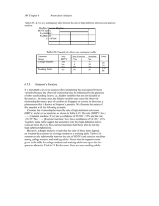
Table 6.19. A two-way contingency table between the sale of high-definition television and exercise
machine.
BuyBuy Exercise Machine
HDTVYesNo
Yes9981180
No5466120
153147300
Table 6.20. Example of a three-way contingency table.
Customer Buy Buy Exercise Machine Total
Group HDTV Yes No
College Students Yes 1 9 10
No 4 30 34
Yes 98 72 170
Working Adult No 50 36 86
6.7.3 Simpson’s Paradox
It is important to exercise caution when interpreting the association between
variables because the observed relationship may be influenced by the presence
of other confounding factors, i.e., hidden variables that are not included in
the analysis. In some cases, the hidden variables may cause the observed
relationship between a pair of variables to disappear or reverse its direction, a
phenomenon that is known as Simpson’s paradox. We illustrate the nature of
this paradox with the following example.
Consider the relationship between the sale of high-definition television
(HDTV) and exercise machine, as shown in Table 6.19. The rule {HDTV=Yes}
−→ {Exercise machine=Yes} has a confidence of 99/180 = 55% and the rule
{HDTV=No} −→ {Exercise machine=Yes} has a confidence of 54/120 = 45%.
Together, these rules suggest that customers who buy high-definition televi-
sions are more likely to buy exercise machines than those who do not buy
high-definition televisions.
However, a deeper analysis reveals that the sales of these items depend
on whether the customer is a college student or a working adult. Table 6.20
summarizes the relationship between the sale of HDTVs and exercise machines
among college students and working adults. Notice that the support counts
given in the table for college students and working adults sum up to the fre-
quencies shown in Table 6.19. Furthermore, there are more working adults

2. 6.7 Evaluation of Association Patterns 385
than college students who buy these items. For college students:
c {HDTV=Yes} −→ {Exercise machine=Yes} = 1/10 = 10%,
c {HDTV=No} −→ {Exercise machine=Yes} = 4/34 = 11.8%,
while for working adults:
c {HDTV=Yes} −→ {Exercise machine=Yes} = 98/170 = 57.7%,
c {HDTV=No} −→ {Exercise machine=Yes} = 50/86 = 58.1%.
The rules suggest that, for each group, customers who do not buy high-
definition televisions are more likely to buy exercise machines, which contradict
the previous conclusion when data from the two customer groups are pooled
together. Even if alternative measures such as correlation, odds ratio, or
interest are applied, we still find that the sale of HDTV and exercise machine
is positively correlated in the combined data but is negatively correlated in
the stratified data (see Exercise 20 on page 414). The reversal in the direction
of association is known as Simpson’s paradox.
The paradox can be explained in the following way. Notice that most
customers who buy HDTVs are working adults. Working adults are also the
largest group of customers who buy exercise machines. Because nearly 85% of
the customers are working adults, the observed relationship between HDTV
and exercise machine turns out to be stronger in the combined data than
what it would have been if the data is stratified. This can also be illustrated
mathematically as follows. Suppose
a/b < c/d and p/q < r/s,
where a/b and p/q may represent the confidence of the rule A −→ B in two
different strata, while c/d and r/s may represent the confidence of the rule
A −→ B in the two strata. When the data is pooled together, the confidence
values of the rules in the combined data are (a + p)/(b + q) and (c + r)/(d + s),
respectively. Simpson’s paradox occurs when
c+ra+p
>,
b+qd+s
thus leading to the wrong conclusion about the relationship between the vari-
ables. The lesson here is that proper stratification is needed to avoid generat-
ing spurious patterns resulting from Simpson’s paradox. For example, market

3. 386 Chapter 6 Association Analysis
4
5
4.5
4
3.5
3
Support
2.5
2
1.5
1
0.5
0
0 500 10001500 2000 2500
Items sorted by support
Figure 6.29. Support distribution of items in the census data set.
basket data from a major supermarket chain should be stratified according to
store locations, while medical records from various patients should be stratified
according to confounding factors such as age and gender.
6.8 Effect of Skewed Support Distribution
The performances of many association analysis algorithms are influenced by
properties of their input data. For example, the computational complexity of
the Apriori algorithm depends on properties such as the number of items in
the data and average transaction width. This section examines another impor-
tant property that has significant influence on the performance of association
analysis algorithms as well as the quality of extracted patterns. More specifi-
cally, we focus on data sets with skewed support distributions, where most of
the items have relatively low to moderate frequencies, but a small number of
them have very high frequencies.
An example of a real data set that exhibits such a distribution is shown in
Figure 6.29. The data, taken from the PUMS (Public Use Microdata Sample)
census data, contains 49,046 records and 2113 asymmetric binary variables.
We shall treat the asymmetric binary variables as items and records as trans-
actions in the remainder of this section. While more than 80% of the items
have support less than 1%, a handful of them have support greater than 90%.

4. 6.8 Effect of Skewed Support Distribution 387
Table 6.21. Grouping the items in the census data set based on their support values.
Group G1 G2 G3
Support < 1% 1% − 90% > 90%
Number of Items 1735 358 20
To illustrate the effect of skewed support distribution on frequent itemset min-
ing, we divide the items into three groups, G1 , G2 , and G3 , according to their
support levels. The number of items that belong to each group is shown in
Table 6.21.
Choosing the right support threshold for mining this data set can be quite
tricky. If we set the threshold too high (e.g., 20%), then we may miss many
interesting patterns involving the low support items from G1 . In market bas-
ket analysis, such low support items may correspond to expensive products
(such as jewelry) that are seldom bought by customers, but whose patterns
are still interesting to retailers. Conversely, when the threshold is set too
low, it becomes difficult to find the association patterns due to the following
reasons. First, the computational and memory requirements of existing asso-
ciation analysis algorithms increase considerably with low support thresholds.
Second, the number of extracted patterns also increases substantially with low
support thresholds. Third, we may extract many spurious patterns that relate
a high-frequency item such as milk to a low-frequency item such as caviar.
Such patterns, which are called cross-support patterns, are likely to be spu-
rious because their correlations tend to be weak. For example, at a support
threshold equal to 0.05%, there are 18,847 frequent pairs involving items from
G1 and G3 . Out of these, 93% of them are cross-support patterns; i.e., the pat-
terns contain items from both G1 and G3 . The maximum correlation obtained
from the cross-support patterns is 0.029, which is much lower than the max-
imum correlation obtained from frequent patterns involving items from the
same group (which is as high as 1.0). Similar statement can be made about
many other interestingness measures discussed in the previous section. This
example shows that a large number of weakly correlated cross-support pat-
terns can be generated when the support threshold is sufficiently low. Before
presenting a methodology for eliminating such patterns, we formally define the
concept of cross-support patterns.

5. 388 Chapter 6 Association Analysis
Definition 6.9 (Cross-Support Pattern). A cross-support pattern is an
itemset X = {i1 , i2 , . . . , ik } whose support ratio
min s(i1 ), s(i2 ), . . . , s(ik )
r(X) = , (6.13)
max s(i1 ), s(i2 ), . . . , s(ik )
is less than a user-specified threshold hc .
Example 6.4. Suppose the support for milk is 70%, while the support for
sugar is 10% and caviar is 0.04%. Given hc = 0.01, the frequent itemset
{milk, sugar, caviar} is a cross-support pattern because its support ratio is
min 0.7, 0.1, 0.00040.0004
r= = 0.00058 < 0.01.=
0.7max 0.7, 0.1, 0.0004
Existing measures such as support and confidence may not be sufficient
to eliminate cross-support patterns, as illustrated by the data set shown in
Figure 6.30. Assuming that hc = 0.3, the itemsets {p, q}, {p, r}, and {p, q, r}
are cross-support patterns because their support ratios, which are equal to
0.2, are less than the threshold hc . Although we can apply a high support
threshold, say, 20%, to eliminate the cross-support patterns, this may come
at the expense of discarding other interesting patterns such as the strongly
correlated itemset, {q, r} that has support equal to 16.7%.
Confidence pruning also does not help because the confidence of the rules
extracted from cross-support patterns can be very high. For example, the
confidence for {q} −→ {p} is 80% even though {p, q} is a cross-support pat-
tern. The fact that the cross-support pattern can produce a high-confidence
rule should not come as a surprise because one of its items (p) appears very
frequently in the data. Therefore, p is expected to appear in many of the
transactions that contain q. Meanwhile, the rule {q} −→ {r} also has high
confidence even though {q, r} is not a cross-support pattern. This example
demonstrates the difficulty of using the confidence measure to distinguish be-
tween rules extracted from cross-support and non-cross-support patterns.
Returning to the previous example, notice that the rule {p} −→ {q} has
very low confidence because most of the transactions that contain p do not
contain q. In contrast, the rule {r} −→ {q}, which is derived from the pattern
{q, r}, has very high confidence. This observation suggests that cross-support
patterns can be detected by examining the lowest confidence rule that can be
extracted from a given itemset. The proof of this statement can be understood
as follows.