Communication Systems

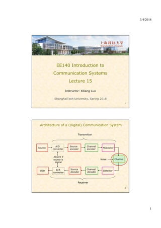
1. 3/4/2018
1
EE140 Introduction to
Communication Systems
Lecture 15
Instructor: Xiliang Luo
ShanghaiTech University, Spring 2018
1
Architecture of a (Digital) Communication System
2
Source
A/D
converter
Source
encoder
Channel
encoder
Modulator
Channel
Detector
Channel
decoder
Source
decoder
D/A
converter
User
Transmitter
Receiver
Absent if
source is
digital
Noise

2. 3/4/2018
2
Contents
• Review: Signal design with zero ISI
• Tx/Rx filter design with channel response
• Equalization
3
Signal Design for Bandlimited Channel
Zero ISI
• Nyquist condition for Zero ISI for pulse shape
1 0
0 0
or ∑ T
• With the above condition, the receiver output
simplifies to
4

3. 3/4/2018
3
Nyquist Condition: Ideal Case
• Nyquist’s first method for eliminating ISI is to use
1 | |
0
/
/
• = Nyquist bandwidth
• The minimum transmission bandwidth for zero ISI.
A channel with bandwidth can support a max.
transmission rate of 2 symbols/sec
5
Achieving Nyquist Condition
• Challenges of designing such or
– ( ) is physically unrealizable due to the abrupt transitions
at
– decays slowly for large t, resulting in little margin of
error in sampling times in the receiver
– This demands accurate sample point timing - a major
challenge in modem / data receiver design
– Inaccuracy in symbol timing is referred to as timing jitter
6

4. 3/4/2018
4
Practical Solution: Raised Cosine Spectrum
• is made up of 3 parts: passband, stopband,
and transition band. The transition band is shaped
like a cosine wave.
7
Time-Domain Pulse Shape
• Taking inverse Fourier transform
8

5. 3/4/2018
5
Contents
• Review: Signal design with zero ISI
• Tx/Rx filter design with channel response
• Equalization
9
Optimum Transmit/Receive Filter
• Recall that when zero-ISI condition is satisfied by
with raised cosine spectrum , then the
sampled output of the receiver filter is
(assume (0)=1)
• Consider binary PAM transmission:
• Variance of noise
with ∗ ∗

10
Error Probability can be minimized through a proper choice
of H f and H f so that / is maximum (assuming H f
fixed and P(f) given)

6. 3/4/2018
6
Optimal Solution
• Compensate the channel distortion equally between
the transmitter and receiver filters
/
/
for
• Then, the transmit signal energy is given by
• Hence
11
By Parseval’s theorem
• Noise variance at the output of the receive filter is
2 2
 ,
Performance loss due to channel distortion
• Special case: 1 for |f|
– This is the ideal case with “flat” fading
– No loss, same as the matched filter receiver for AWGN
channel
12
Optimal Solution (cont’d)

7. 3/4/2018
7
Exercise
• Determine the optimum transmitting and receiving
filters for a binary communications system that
transmits data at a rate R=1/T = 4800 bps over a
channel with a frequency response ;
|f| ≤W where W= 4800 Hz
• The additive noise is zero-mean white Gaussian
with spectral density 2
⁄ 10 Watt/Hz
• Determine the required transmit energy to achieve
10
13
Solution
• Since W = 1/T = 4800, we use a signal pulse with a
raised cosine spectrum and a roll-off factor = 1
• Thus,
1
2
1 cos | | cos
| |
9600
• Therefore
cos
9600
1
4800
, for |f| 4800
• One can now use these filters to determine the
amount of transmit energy required to achieve a
specified error probability
14

8. 3/4/2018
8
Performance with ISI
• If zero-ISI condition is not met, then
• Let
• Then
15
• Often only 2 significant terms are considered.
• Finding the probability of error in this case is quite
difficult. Various approximation can be used
(Gaussian approximation, Chernoff bound, etc.)
• What is the solution?
16
Performance with ISI

9. 3/4/2018
9
Monte Carlo Simulation
17
• If one wants to be within 10% accuracy, how
many independent simulation runs do we need?
• If ~10 (this is typically the case for optical
communication systems), and assume each
simulation run takes 1 msec, how long will the
simulation take?
18
Monte Carlo Simulation (cont’d)

10. 3/4/2018
10
Contents
• Review: Signal design with zero ISI
• Tx/Rx filter design with channel response
• Equalization
19
What is Equalizer
• We have shown that
– By properly designing the transmitting and receiving filters,
one can guarantee zero ISI at sampling instants, thereby
minimizing .
– Appropriate when the channel is precisely known and its
characteristics do not change with time
– In practice, the channel is unknown or time-varying
• Channel equalizer: a receiving filter with adjustable
frequency response to minimize/eliminate inter-
symbol interference
20

11. 3/4/2018
11
Equalizer Configuration
• Overall frequency response
• Nyquist criterion for zero-ISI
• Ideal zero-ISI equalizer is an inverse channel filter
with
∝
1
| | 1/2
21
Linear Transversal Filter
• Finite impulse response (FIR) filter
• are the adjustable 2N+1 equalizer coefficients
• N is sufficiently large to span the length of ISI
22

12. 3/4/2018
12
Zero-Forcing Equalizer
• : received pulse from a channel to be equalized
• ∑
1, 0
0, 1, … ,
To suppose 2N adjacent interference terms
23
Zero-Forcing Equalizer (cont’d)
• Rearrange to matrix form
24

13. 3/4/2018
13
Example
25
Solution
26

14. 3/4/2018
14
Solution
• The inverse of this matrix (e.g by MATLAB)
• Therefore
0.117, 0.158, 0.937, 0.133, 0.091
• Equalized pulse response
• It can be verified that
0 1.0 0, 1, 2
27
Solution
• Note that values of for 2 or 2 are not
zero. For example:
28

15. 3/4/2018
15
Minimum Mean-Square Error Equalizer
• Drawback of ZF equalizer
– Ignores the additive noise
– May even amplify the noise power
• Alternatively,
– Relax zero ISI condition
– Minimize the combined power in the residual ISI and
additive noise at the output of the equalizer
• MMSE equalizer:
– a channel equalizer that is optimized based on the
minimum mean-square error (MMSE) criterion
29
MMSE Criterion
• The output is sampled at :
• Let A = desired equalizer output
≜ Minimum
30

16. 3/4/2018
16
MMSE Criterion (cont’d)
2
where
• MMSE solution is obtained by 0
, 0, 1, … ,
31
E is taken over
and the additive noise
MMSE Equalizer vs. ZF Equalizer
• Both can be obtained by solving similar equations
• ZF equalizer does not consider effects of noise
• MMSE equalizer designed so that mean-square error
(consisting of ISI terms and noise at the equalizer
output) is minimized
• Both equalizers are known as linear equalizers
32

17. 3/4/2018
17
Decision Feedback Equalizer (DFE)
• DFE is a nonlinear equalizer which attempts to
subtract from the current symbol to be detected the
ISI created by previously detected symbols
33
Examples of Channels with ISI
34

18. 3/4/2018
18
Frequency Response
35
Channel B tends to significantly enhance the noise when a
linear equalizer is used (since linear equalizers have to
introduce a large gain to compensate for channel null).
Performance of MMSE Equalizer
36

19. 3/4/2018
19
Performance of DFE
37
Maximum Likelihood Sequence Estimation
(MLSE)
• Let the transmitting filter have a square root raised cosine
frequency response
| |
0
• The receiving filter is matched to the transmitter filter with
| |
0
• The sampled output from receiving filter is
38

20. 3/4/2018
20
MLSE
• Assume ISI affects finite number of symbols, with
0
• Then, the channel is equivalent to an FIR discrete-
time filter
39
Performance of MLSE
40

21. 3/4/2018
21
41
More about Equalization
Thanks for your kind attention!
Questions?
42