
Recommended
Recommended
More Related Content
Similar to 2eda79c41aee471db842e8df57d4143f_7317.docYour temporary usag.docx
Similar to 2eda79c41aee471db842e8df57d4143f_7317.docYour temporary usag.docx (20)
More from gilbertkpeters11344
More from gilbertkpeters11344 (20)
Recently uploaded
Recently uploaded (20)
2eda79c41aee471db842e8df57d4143f_7317.docYour temporary usag.docx
- 1. 2eda79c41aee471db842e8df57d4143f_7317.doc Your temporary usage period for IBM SPSS Statistics will expire in 13 days. GET FILE='C:Documents and SettingsAdministratorDesktop3303_Assign_December2014.sa v'. DATASET NAME DataSet1 WINDOW=FRONT. UNIANOVA amount BY stomach weight /METHOD=SSTYPE(3) /INTERCEPT=INCLUDE /PLOT=PROFILE(weight*stomach) /PRINT=ETASQ DESCRIPTIVE /CRITERIA=ALPHA(.05) /DESIGN=stomach weight stomach*weight. Univariate Analysis of Variance Notes Output Created 23-DEC-2014 19:40:40 Comments Input Data C:Documents and
- 2. SettingsAdministratorDesktop3303_Assign_December2014.sa v Active Dataset DataSet1 Filter <none> Weight <none> Split File <none> N of Rows in Working Data File 78 Missing Value Handling Definition of Missing User-defined missing values are treated as missing. Cases Used Statistics are based on all cases with valid data for all variables in the model. Syntax UNIANOVA amount BY stomach weight /METHOD=SSTYPE(3) /INTERCEPT=INCLUDE /PLOT=PROFILE(weight*stomach) /PRINT=ETASQ DESCRIPTIVE /CRITERIA=ALPHA(.05) /DESIGN=stomach weight stomach*weight. Resources Processor Time 00:00:01.38
- 3. Elapsed Time 00:00:02.16 [DataSet1] C:Documents and SettingsAdministratorDesktop3303_Assign_December2014.sa v Between-Subjects Factors Value Label N stomach 1 empty 39 2 full 39 weight 1 underweight 26 2 normal 26 3 overweight 26
- 4. Descriptive Statistics Dependent Variable: amount stomach weight Mean Std. Deviation N empty underweight 24.92 5.330 13 normal 30.54 1.984 13 overweight 25.38 5.455 13 Total 26.95 5.124 39 full underweight 14.00 2.517 13 normal 12.00 1.472
- 5. 13 overweight 22.77 6.796 13 Total 16.26 6.303 39 Total underweight 19.46 6.906 26 normal 21.27 9.606 26 overweight 24.08 6.183 26 Total 21.60 7.843 78 Tests of Between-Subjects Effects Dependent Variable: amount Source
- 6. Type III Sum of Squares df Mean Square F Sig. Partial Eta Squared Corrected Model 3335.141a 5 667.028 34.267 .000 .704 Intercept 36400.321 1 36400.321 1869.962 .000 .963 stomach 2229.346 1 2229.346 114.526 .000 .614 weight 281.256 2 140.628 7.224 .001 .167 stomach * weight 824.538
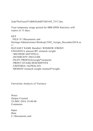
- 7. 2 412.269 21.179 .000 .370 Error 1401.538 72 19.466 Total 41137.000 78 Corrected Total 4736.679 77 a. R Squared = .704 (Adjusted R Squared = .684) Profile Plots
- 8. SORT CASES BY stomach. SPLIT FILE LAYERED BY stomach. ONEWAY amount BY weight /MISSING ANALYSIS /POSTHOC=TUKEY ALPHA(0.05). Oneway Notes Output Created 23-DEC-2014 20:26:34 Comments Input Data C:Documents and SettingsAdministratorDesktop3303_Assign_December2014.sa v Active Dataset DataSet1 Filter <none> Weight <none> Split File stomach
- 9. N of Rows in Working Data File 78 Missing Value Handling Definition of Missing User-defined missing values are treated as missing. Cases Used Statistics for each analysis are based on cases with no missing data for any variable in the analysis. Syntax ONEWAY amount BY weight /MISSING ANALYSIS /POSTHOC=TUKEY ALPHA(0.05). Resources Processor Time 00:00:00.03 Elapsed Time 00:00:00.04 [DataSet1] C:Documents and SettingsAdministratorDesktop3303_Assign_December2014.sa v ANOVA amount stomach Sum of Squares df Mean Square F Sig.
- 10. empty Between Groups 252.667 2 126.333 6.103 .005 Within Groups 745.231 36 20.701 Total 997.897 38 full Between Groups 853.128 2 426.564 23.398 .000 Within Groups 656.308 36 18.231
- 11. Total 1509.436 38 Post Hoc Tests Multiple Comparisons Dependent Variable: amount Tukey HSD stomach (I) weight (J) weight Mean Difference (I-J) Std. Error Sig. 95% Confidence Interval Lower Bound empty underweight normal -5.615* 1.785 .009
- 14. normal 10.769* 1.675 .000 6.68 Multiple Comparisons Dependent Variable: amount Tukey HSD stomach (I) weight (J) weight 95% Confidence Interval Upper Bound empty underweight normal -1.25* overweight 3.90 normal underweight 9.98* overweight 9.52* overweight
- 15. underweight 4.82 normal -.79* full underweight normal 6.09 overweight -4.68* normal underweight 2.09 overweight -6.68* overweight underweight 12.86* normal 14.86* *. The mean difference is significant at the 0.05 level. Homogeneous Subsets
- 16. amount stomach=empty Tukey HSD weight N Subset for alpha = 0.05 1 2 underweight 13 24.92 overweight 13 25.38 normal 13 30.54 Sig. .964 1.000 Means for groups in homogeneous subsets are displayed. a. Uses Harmonic Mean Sample Size = 13.000.
- 17. stomach=full Tukey HSD weight N Subset for alpha = 0.05 1 2 normal 13 12.00 underweight 13 14.00 overweight 13 22.77 Sig. .464 1.000 Means for groups in homogeneous subsets are displayed. a. Uses Harmonic Mean Sample Size = 13.000. 69ad4fe0057b4f49987aec1db0c5143e_7317.doc SPLIT FILE OFF. ONEWAY amount BY VAR00001
- 18. /MISSING ANALYSIS /POSTHOC=TUKEY ALPHA(0.05). Oneway Notes Output Created 23-DEC-2014 20:53:29 Comments Input Data C:Documents and SettingsAdministratorDesktop3303_Assign_December2014.sa v Active Dataset DataSet1 Filter <none> Weight <none> Split File <none> N of Rows in Working Data File 79 Missing Value Handling
- 19. Definition of Missing User-defined missing values are treated as missing. Cases Used Statistics for each analysis are based on cases with no missing data for any variable in the analysis. Syntax ONEWAY amount BY VAR00001 /MISSING ANALYSIS /POSTHOC=TUKEY ALPHA(0.05). Resources Processor Time 00:00:00.01 Elapsed Time 00:00:00.02 [DataSet1] C:Documents and SettingsAdministratorDesktop3303_Assign_December2014.sa v ANOVA amount Sum of Squares df Mean Square F Sig. Between Groups 3335.141 5 667.028
- 20. 34.267 .000 Within Groups 1401.538 72 19.466 Total 4736.679 77 Post Hoc Tests Multiple Comparisons Dependent Variable: amount Tukey HSD (I) VAR00001 (J) VAR00001 Mean Difference (I-J) Std. Error Sig. 95% Confidence Interval Lower Bound
- 26. .813 -7.22 2.91 2.00 8.769* 1.731 .000 3.70 13.84 3.00 -7.769* 1.731 .000 -12.84 -2.70 4.00 10.769* 1.731 .000 5.70 15.84 5.00 -2.615 1.731 .658 -7.68 2.45 *. The mean difference is significant at the 0.05 level.
- 27. Homogeneous Subsets amount Tukey HSD VAR00001 N Subset for alpha = 0.05 1 2 3 4.00 13 12.00 2.00 13 14.00 6.00 13 22.77 1.00 13 24.92 5.00 13
- 28. 25.38 3.00 13 30.54 Sig. .856 .658 1.000 Means for groups in homogeneous subsets are displayed. a. Uses Harmonic Mean Sample Size = 13.000. 882e7dac74da4c11b802bd3ffa5347b7_7317.pdf PSY3303 Assignment p. 1 Edith Cowan University Faculty of Health, Engineering and Science School of Psychology
- 29. and Social Science PSY3303 Research Applications and Ethical Issues Assignment December 2014 PSY3303 Assignment p. 2 Section A: One way and Factorial ANOVAs Total Points for Section A = 96 Assignments are to be handed in directly to your TUTOR. Part 1: Background
- 30. In 1968, Schachter published one of the first studies on obesity and eating behaviour. The theory that emerged from this literature was that overweight individuals do not respond to their internal, biological signals of hunger in the same way that normal weight and underweight people do. In other words, people who are overweight tend to eat regardless of whether or not they are hungry. In Schachter’s paradigm, participants were told that they were participating in a “taste test”. Each participant came to the laboratory after fasting for 12 hours. Just before the “taste test”, half the participants were given a full meal and could eat as much as they wanted, and half were not given any food at all. One hour later, a range of hors d’oeuvres were spread out on a table in front of the participant. The participant was asked to provide a rating on a scale of 0 (yucky) to 5 (extremely delicious) for each type of hors d’oeuvre. The experimenter then left the room so that the participant could “taste test” in private. After the participant finished their task, Schachter measured the amount of food (in grams) eaten by the participants. The data are presented in an SPSS file named <3303_Assign_December2014.sav> located in the PSY3303 Blackboard site under “Assignments”. It is in your best interests to spend some time getting to know how the file was set up and deciding for yourself how to add variables to the file in order to perform some of the analyses required. Make sure you know what each of the following variables and
- 31. their values represent in the factorial design. For example, for the variable Stomach, the Value=1 represents ‘empty’ hence the scores which have this value represent the empty stomach condition. PSY3303 Assignment p. 3 Student Name: Tutor’s Name: Part 2: Assignment Task Conduct the appropriate SPSS analyses to answer the following questions. 1. Complete the following Summary Table. (2 points) Source SS df MS F Stomach Weight
- 32. Stomach × Weight Error Total PSY3303 Assignment p. 4 2. Calculate η2 for the main effects and the interaction in the space below. In doing so, do not rely on the SPSS output which provides different values to what are typically reported. (3 points)
- 33. 3. Conduct a (post hoc) pairwise analysis of the group cell means. Which of these post hoc contrasts are significant? (use α = 0.05) (Circle the appropriate response) (4 points) Empty+Underweight vs Full+Underweight Yes No Empty+Normal vs Full+Normal Yes No Full+Underweight vs Full+Overweight Yes No Empty+Overweight vs Full+Overweight Yes No 4. The interaction in the ANOVA suggests that it would be useful to examine simple main effects. Conduct the appropriate analyses to determine if there is an effect of weight on a participant with an empty stomach and an effect of weight on a participant with a full stomach. Provide the following details of these effects. (2 points) F weight.empty only = , df = , , p < F weight.full only = , df = , , p <
- 34. PSY3303 Assignment p. 5 5. Write up the analyses as you would in the Results and Discussion section of a journal article. In the Results section (40 points), you should include the report of the central tendency, variability measures, outcomes of the relevant ANOVAs (including the eta- squared results (and what they suggest) and the simple effects analyses (and what they indicate). You should also include a graph of the data (15 points). In your Discussion section (30 points), you should briefly describe the pattern of differences for the two stomach conditions. Discuss what is surprising about these data and the pattern they show, especially with respect to what Schachter says about the overweight subjects (Hint: It may be useful to carefully consider the interaction as shown on the graph.). Also in the Discussion section, and with respect to the data and the analyses you have carried out, describe the relationship between weight and eating behaviours. (Hint: Consider whether or not Schachter’s theory is supported by the data. It may be useful to consider the eta-squared results again.). NOTE: You do not have to find additional references on obesity and the effects of eating behaviour to write the Discussion section. Please read the following formatting instructions. The Results and Discussion section of Part A has a THREE (3) page limit. Failure to read and understand these instructions will lead to lost
- 35. marks! • The Results and Discussion section must be formatted according to APA style and typed on A4 paper. No handwritten assignments will be accepted. Use Times or Times New Roman 12-point font (Times is the font used in this assignment), double-spaced, with 2.5- cm margins left and right, top and bottom. If you follow these instructions, you should have a maximum of 25 lines per A4 page. In other words, do not include more than 25 lines per A4 page. • Your Results and Discussion section should be no more than THREE (3) pages long. If you go over the 3-page limit or format your Results and Discussion section in a way that looks like it goes over the 3-page limit, then the lines you write in excess of the 3-page limit will not be read. In addition, you will be automatically penalised a minimum of 10 points. No appeals – none whatsoever, for any possible reason – to this automatic 10-point penalty will be accepted. • The graph must be formatted in APA style, with an appropriate APA-formatted caption and may be either hand-drawn or computer-drawn. The graph must be formatted within the 3-page Results and Discussion section, just like it would appear in a journal article. To be clear and unambiguous: Everything you write in your Results and Discussion section for
- 36. Part A – headings, graph, words, anything – must be within the 3-page limit. Do not include anything in an Appendix. End of Section A PSY3303 Assignment p. 6 Section B: One way and Factorial ANOVAs Total Points for Section B = 95 Assignments are to be handed in directly to your TUTOR. Part 1: Background A psychologist was interested in the effects of room temperature on aggression. In particular, does an increase in temperature lead to an increase in aggressive behaviour, and if so, are males and females affected equally? The psychologist tested participants in a laboratory, where the room temperature could be controlled precisely. Participants were required to make a telephone call to a given number in order to obtain some information about an insurance claim. The person on the other end of the call was a confederate of the experimenter who played the role of an obtuse, unhelpful insurance clerk. Each phone call was recorded and two independent judges, unaware of experimental condition, rated each exchange in terms of the level of aggression displayed by the participant. Aggression was rated on a scale of 0 (no
- 37. aggression) to 100 (extremely aggressive). 40 females and 40 males were tested, with 10 from each gender randomly allocated to each of the four room temperature conditions (25, 30, 35, 40 degrees celsius). The following data was collected. The values represent the average of the two judges ratings for each participant. Temperature (deg C) Gender 25 30 35 40 Males 57 58 70 61 62 65 64 66 69 60 62 68 65 66 64 70 63 59 60 65
- 38. 62 69 68 67 65 67 64 63 72 60 68 74 72 69 67 65 78 65 66 71 Females 58 56 62 58 55 53 58 61 54 56
- 40. PSY3303 Assignment p. 7 Part B, Section 2: Assignment Task (Factorial ANOVA & Post Hocs) Student Name: Conduct the appropriate SPSS analyses to answer the following questions in the spaces provided. 1. Fill in the blanks (be specific) (6 points) Independent Variable #1 Independent Variable #2 Dependent Variable: 2. Formulate the research question being asked in this study as concisely as you can, making sure that you mention the dependent variable and what the two independent variables (and their levels) are. (4 points)
- 41. 3. For each cell, supply the information required in the spaces below (to two decimal places). (1 point) Temperature (degrees C) Gender 25 30 35 40 Males Mean=________ Std Dev=_______ Mean=________ Std Dev=_______ Mean=________ Std Dev=_______
- 42. Mean=________ Std Dev=_______ Females Mean=________ Std Dev=_______ Mean=________ Std Dev=_______ Mean=________ Std Dev=_______ Mean=________ Std Dev=_______
- 43. PSY3303 Assignment p. 8 4. Complete the following Summary Table. (2 points) Source SS Df MS F Gender Temperature Gender × Temperature Error Total 5. Calculate η2 for the main effects and the interaction in the space below. In doing so, do not rely on the SPSS output which provides different values to what are
- 44. typically reported. It is suggested that manual calculations be conducted from the above table. (3 points) PSY3303 Assignment p. 9 6. Conduct a (post hoc) pairwise analysis of the group cell means. Which of these post hoc contrasts are significant (use α = 0.05)? (Circle the appropriate
- 45. response) (4 points) Male-25 vs. Female-25 Yes No Male-30 vs. Female-30 Yes No Male-35 vs. Female-35 Yes No Male-40 vs. Female-40 Yes No 7. Write up the analyses as you would in the Results section of a journal article, including the report of the central tendency and variability measures and the outcome of the analyses (30 points). Include a graph of the data in your Results section (15 points). Follow this up with a Discussion section (30 points) in which you present some conclusions about the relationship between gender and temperature on aggression. NOTE: You do not have to find additional references on the effects of gender and temperature on aggression to write the Discussion section. Please read the following formatting instructions. The Results and Discussion section of Part B has a THREE (3) page limit. Failure to read and understand these instructions will lead to lost marks! • The Results and Discussion section must be formatted according to APA style and typed on A4 paper. No handwritten assignments will be accepted. Use Times or Times New Roman 12-point font (Times is the font used in this
- 46. assignment), double-spaced, with 2.5- cm margins left and right, top and bottom. If you follow these instructions, you should have a maximum of 25 lines per A4 page. In other words, do not include more than 25 lines per A4 page. • Your Results and Discussion section should be no more than THREE (3) pages long. If you go over the 3-page limit or format your Results and Discussion section in a way that looks like it goes over the 3-page limit, then the lines you write in excess of the 3-page limit will not be read. In addition, you will be automatically penalised a minimum of 10 points. No appeals – none whatsoever, for any possible reason – to this automatic 10-point penalty will be accepted. • The graph must be formatted in APA style, with an appropriate APA-formatted caption and may be either hand-drawn or computer-drawn. The graph must be formatted within the 3-page Results and Discussion section, just like it would appear in a journal article. To be clear and unambiguous: Everything you write in your Results and Discussion section for Part B – headings, graph, words, anything – must be within the 3-page limit. Do not include anything in an Appendix. End of the Assignment
- 47. PSY3303 Assignment p. 10 APPENDIX FOR THE ASSIGNMENT RECOMMENDATIONS FOR RESULTS REPORTING The best tip that I can provide psychology students regarding APA formatting is to go onto the APA website (www.apa.org) and visit the journals section. Here, you can survey a range of APA journals (i.e., journals with the APA logo or brand on them). Feel free to download as many of these journal articles as you like – in fact, I encourage you to do so. By looking at the way that the Results and Discussion sections are formatted in these APA- branded journal articles, you will get guidance on how it is done properly. In the Results section of the report you should take note of the following points: 1. The statistical procedures that were conducted are reported and the statistical outcomes obtained. The results are not interpreted in this section of the report. However, you may say things like: “...there was a significant difference between the means of high and low motivation groups, with the high motivation group performing significantly more effectively than the low motivation group F(1, 29) = 43.56, p < .05. This supports the prediction of the study concerning the positive effect that high motivation would have on efficiency.” The
- 48. order in which the analyses are reported should approximate the order in which they were conducted: A. When introducing your analyses, describe how the DV was measured. For example, a score of 1 may be given to a correct response and a score of 0 to an incorrect response. In more complex procedures a score of 1 to 5 may be given, with 1 indicating low motivation and 5 high motivation. (The reader needs this sort of information to allow him/her to interpret the findings.) The assumptions of the analyses are also important here. For example, you may say that all data met the requirements of normality and homogeneity of variance for the performance of the parametric procedures to be used. B. This initial analysis reported is always the descriptive statistics that summarise or describe the relationships obtained. These should be presented in table or graphical form, whichever is most explanatory. When means are reported the standard deviation should also be reported for each condition. When describing these results, refer to the table or figure (you do not have to put all the mean scores in the text of the report.) You should, however, report the most important finding or anything unusual, such as a large standard deviation on a single condition. C. Perform the required inferential procedures. The formal name of the procedure is presented and how it is applied to the data. The results of the
- 49. analysis is reported, using the statistic and the α level employed. For example, F (1,56) = 5.94, p < .05. You also report whether this result is significant and the effect size (if you have it). D. At this point a supplementary analysis is often conducted. This may reflect specific research hypotheses that were posed in the Introduction. The specific procedure is reported (e.g., a priori contrast or post hoc analysis). When reporting effects, you should always tell the reader what descriptive statistics you are testing, so that they can follow what you are reporting. With post hoc analysis you may present a table of the pairs, with significance reported with an asterisk. 3. You should not talk about “very significant” or “highly significant” results. The results are either significant or not. Sometimes a researcher will suggest that the results point towards a significant effect, when a p value lies between 0.051 and 0.09. In reporting this sort of effect it should have special significance to your research and be a point which will be discussed in the Discussion section. PSY3303 Assignment p. 11 4. When figures are presented, they should be accompanied by a caption in which the author
- 50. should tell the reader something about the figure. You should not just call it Figure 1. 5. A table is used when it is important for the reader to compare the actual numerical values of the presented data, when there are too many numbers to include all the means individually in the body of the text, or there are too many numbers to place in an explanatory fashion on a figure. As with figures, the reader is directed to the relevant table in the body of the results. These are general pointers only. Many methods books and the APA manual will give you further information. A good strategy is to look at several research articles. While all will present information slightly differently, the same general structure will be used. Methods books often give an example of a research report and provide information concerning positive aspects of the writing with it. The articles you have used in previous evaluation exercises should also be rescrutinised with special emphasis on the Method and Results sections. A word of caution: Often you will see a double line with “Insert Table 1 about here”, or similar. This is done for publication purposes only. When you are writing a report, do not do this. Insert a figure or a table into the appropriate location. When describing this in the text direct the reader to its location by label only (i.e., In Figure 1.....). cd07be3b913747ee9f8d1a2f8352b719_7317.pdf
- 51. Univariate Analysis of Variance Notes Output Created Comments Input Data Active Dataset Filter Weight Split File Missing Value Handling Definition of Missing Cases Used Syntax Resources Processor Time Elapsed Time 30-DEC-2014 14:27:54 DataSet0 <none> <none>
- 52. <none> 80 00:00:02.78 00:00:03.02 Between-Subjects Factors Value Label N Temp 1 2 3 4 Gender 1 2 25 20 30 20 35 20 40 20 Male 40 Female 40
- 53. Page 1 Descriptive Statistics Dependent Variable: AggressionDependent Variable: AggressionDependent Variable: Aggression Temp Gender Dependent Variable: Aggression Mean Std. Deviation N 25 Male Female Total 30 Male Female Total 35 Male Female Total 40 Male Female
- 54. Total Total Male Female Total 63.2000 4.39191 10 57.1000 2.88483 10 60.1500 4.78237 20 64.2000 3.39280 10 61.9000 4.25441 10 63.0500 3.92663 20 65.7000 3.59166 10 69.0000 4.78423 10 67.3500 4.45179 20 69.5000 4.24918 10 76.1000 4.81779 10 72.8000 5.56871 20 65.6500 4.48673 40 66.0250 8.35583 40
- 55. 65.8375 6.66645 80 Dependent Variable: AggressionDependent Variable: Aggression Tests of Between-Subjects Effects Dependent Variable: AggressionDependent Variable: AggressionDependent Variable: Aggression Source Dependent Variable: Aggression df Mean Square F Sig. Corrected Model Intercept Temp Gender Temp * Gender Error Total Corrected Total 2302.387a 7 328.912 19.596 .000 346766.112 1 346766.112 20659.628 .000
- 56. 1817.637 3 605.879 36.097 .000 2.813 1 2.813 .168 .684 481.937 3 160.646 9.571 .000 1208.500 72 16.785 350277.000 80 3510.887 79 Dependent Variable: AggressionDependent Variable: Aggression a. Post Hoc Tests Temp Page 2 Multiple Comparisons Dependent Variable: AggressionDependent Variable: Aggression Tukey HSDTukey HSD (I) Temp (J) Temp Tukey HSD
- 57. Std. Error Sig. 95% Confidence Interval Lower Bound Upper Bound 25 30 35 40 30 25 35 40 35 25 30 40 40 25 30 35 -2.9000 1.29556 .123 -6.3074 .5074 -7.2000* 1.29556 .000 -10.6074 -3.7926 -12.6500* 1.29556 .000 -16.0574 -9.2426
- 58. 2.9000 1.29556 .123 -.5074 6.3074 -4.3000* 1.29556 .008 -7.7074 -.8926 -9.7500* 1.29556 .000 -13.1574 -6.3426 7.2000* 1.29556 .000 3.7926 10.6074 4.3000* 1.29556 .008 .8926 7.7074 -5.4500* 1.29556 .000 -8.8574 -2.0426 12.6500* 1.29556 .000 9.2426 16.0574 9.7500* 1.29556 .000 6.3426 13.1574 5.4500* 1.29556 .000 2.0426 8.8574 Tukey HSDTukey HSD *. Profile Plots Page 3 Temp 40353025 E s ti
- 59. m a te d M a rg in a l M e a n s 80.00 75.00 70.00 65.00 60.00 55.00 Estimated Marginal Means of Aggression Female
- 60. Male Gender Oneway Page 4 Notes Output Created Comments Input Data Active Dataset Filter Weight Split File Missing Value Handling Definition of Missing Cases Used Syntax Resources Processor Time Elapsed Time
- 61. 30-DEC-2014 14:28:58 DataSet0 <none> <none> <none> 80 00:00:00.05 00:00:00.05 Page 5 Descriptives AggressionAggressionAggressionAggression N Mean Std. Deviation Std. Error Lower Bound Upper Bound 25Male 25Female 30Male 30Female 35Male
- 62. 35Female 40Male 40Female Total 10 63.2000 4.39191 1.38884 60.0582 66.3418 57.00 10 57.1000 2.88483 .91226 55.0363 59.1637 53.00 10 64.2000 3.39280 1.07290 61.7729 66.6271 59.00 10 61.9000 4.25441 1.34536 58.8566 64.9434 56.00 10 65.7000 3.59166 1.13578 63.1307 68.2693 60.00 10 69.0000 4.78423 1.51291 65.5776 72.4224 62.00 10 69.5000 4.24918 1.34371 66.4603 72.5397 65.00 10 76.1000 4.81779 1.52352 72.6536 79.5464 69.00 80 65.8375 6.66645 .74533 64.3540 67.3210 53.00 Aggression Aggression Descriptives AggressionAggressionAggressionAggression Minimum Maximum 25Male
- 63. 25Female 30Male 30Female 35Male 35Female 40Male 40Female Total 57.00 70.00 53.00 62.00 59.00 70.00 56.00 70.00 60.00 72.00 62.00 77.00 65.00 78.00 69.00 84.00 53.00 84.00 Aggression Aggression
- 64. ANOVA AggressionAggressionAggressionAggression df Mean Square F Sig. Between Groups Within Groups Total 2302.387 7 328.912 19.596 .000 1208.500 72 16.785 3510.887 79 AggressionAggression Post Hoc Tests Page 6 Multiple Comparisons Dependent Variable: AggressionDependent Variable: Aggression Tukey HSDTukey HSD (I) Cell (J) Cell Tukey HSD
- 65. Std. Error Sig. 95% Confidence Interval Lower Bound Upper Bound 25Male 25Female 30Male 30Female 35Male 35Female 40Male 40Female 25Female 25Male 30Male 30Female 35Male 35Female 40Male 40Female 30Male 25Male
- 67. 40Male 40Female 6.10000* 1.83220 .028 .3802 11.8198 -1.00000 1.83220 .999 -6.7198 4.7198 1.30000 1.83220 .996 -4.4198 7.0198 -2.50000 1.83220 .870 -8.2198 3.2198 -5.80000* 1.83220 .045 -11.5198 -.0802 -6.30000* 1.83220 .021 -12.0198 -.5802 -12.90000* 1.83220 .000 -18.6198 -7.1802 -6.10000* 1.83220 .028 -11.8198 -.3802 -7.10000* 1.83220 .005 -12.8198 -1.3802 -4.80000 1.83220 .166 -10.5198 .9198 -8.60000* 1.83220 .000 -14.3198 -2.8802 -11.90000* 1.83220 .000 -17.6198 -6.1802 -12.40000* 1.83220 .000 -18.1198 -6.6802 -19.00000* 1.83220 .000 -24.7198 -13.2802 1.00000 1.83220 .999 -4.7198 6.7198 7.10000* 1.83220 .005 1.3802 12.8198
- 68. 2.30000 1.83220 .912 -3.4198 8.0198 -1.50000 1.83220 .992 -7.2198 4.2198 -4.80000 1.83220 .166 -10.5198 .9198 -5.30000 1.83220 .089 -11.0198 .4198 -11.90000* 1.83220 .000 -17.6198 -6.1802 -1.30000 1.83220 .996 -7.0198 4.4198 4.80000 1.83220 .166 -.9198 10.5198 -2.30000 1.83220 .912 -8.0198 3.4198 -3.80000 1.83220 .441 -9.5198 1.9198 -7.10000* 1.83220 .005 -12.8198 -1.3802 -7.60000* 1.83220 .002 -13.3198 -1.8802 -14.20000* 1.83220 .000 -19.9198 -8.4802 2.50000 1.83220 .870 -3.2198 8.2198 8.60000* 1.83220 .000 2.8802 14.3198 1.50000 1.83220 .992 -4.2198 7.2198 3.80000 1.83220 .441 -1.9198 9.5198 -3.30000 1.83220 .621 -9.0198 2.4198 -3.80000 1.83220 .441 -9.5198 1.9198
- 69. -10.40000* 1.83220 .000 -16.1198 -4.6802 5.80000* 1.83220 .045 .0802 11.5198 Tukey HSDTukey HSD Page 7 Multiple Comparisons Dependent Variable: AggressionDependent Variable: Aggression Tukey HSDTukey HSD (I) Cell (J) Cell Tukey HSD Std. Error Sig. 95% Confidence Interval Lower Bound Upper Bound 35Female 25Male 25Female 30Male 30Female 35Male
- 70. 40Male 40Female 40Male 25Male 25Female 30Male 30Female 35Male 35Female 40Female 40Female 25Male 25Female 30Male 30Female 35Male 35Female 40Male 5.80000* 1.83220 .045 .0802 11.5198 11.90000* 1.83220 .000 6.1802 17.6198
- 71. 4.80000 1.83220 .166 -.9198 10.5198 7.10000* 1.83220 .005 1.3802 12.8198 3.30000 1.83220 .621 -2.4198 9.0198 -.50000 1.83220 1.000 -6.2198 5.2198 -7.10000* 1.83220 .005 -12.8198 -1.3802 6.30000* 1.83220 .021 .5802 12.0198 12.40000* 1.83220 .000 6.6802 18.1198 5.30000 1.83220 .089 -.4198 11.0198 7.60000* 1.83220 .002 1.8802 13.3198 3.80000 1.83220 .441 -1.9198 9.5198 .50000 1.83220 1.000 -5.2198 6.2198 -6.60000* 1.83220 .013 -12.3198 -.8802 12.90000* 1.83220 .000 7.1802 18.6198 19.00000* 1.83220 .000 13.2802 24.7198 11.90000* 1.83220 .000 6.1802 17.6198 14.20000* 1.83220 .000 8.4802 19.9198 10.40000* 1.83220 .000 4.6802 16.1198 7.10000* 1.83220 .005 1.3802 12.8198
- 72. 6.60000* 1.83220 .013 .8802 12.3198 Tukey HSDTukey HSD *. Oneway Page 8 Notes Output Created Comments Input Data Active Dataset Filter Weight Split File Missing Value Handling Definition of Missing Cases Used Syntax Resources Processor Time
- 73. Elapsed Time 30-DEC-2014 14:32:50 DataSet0 <none> <none> Gender 80 00:00:00.03 00:00:00.03 Page 9 Descriptives AggressionAggressionAggression Gender Aggression N Mean Std. Deviation Std. Error Lower Bound Upper Bound Male 25 30
- 74. 35 40 Total Female 25 30 35 40 Total 10 63.2000 4.39191 1.38884 60.0582 66.3418 57.00 10 64.2000 3.39280 1.07290 61.7729 66.6271 59.00 10 65.7000 3.59166 1.13578 63.1307 68.2693 60.00 10 69.5000 4.24918 1.34371 66.4603 72.5397 65.00 40 65.6500 4.48673 .70941 64.2151 67.0849 57.00 10 57.1000 2.88483 .91226 55.0363 59.1637 53.00 10 61.9000 4.25441 1.34536 58.8566 64.9434 56.00 10 69.0000 4.78423 1.51291 65.5776 72.4224 62.00 10 76.1000 4.81779 1.52352 72.6536 79.5464 69.00 40 66.0250 8.35583 1.32117 63.3527 68.6973 53.00
- 75. Aggression Aggression Descriptives AggressionAggressionAggression Gender Aggression Minimum Maximum Male 25 30 35 40 Total Female 25 30 35 40 Total 57.00 70.00 59.00 70.00
- 76. 60.00 72.00 65.00 78.00 57.00 78.00 53.00 62.00 56.00 70.00 62.00 77.00 69.00 84.00 53.00 84.00 Aggression Aggression Page 10 ANOVA AggressionAggressionAggression Gender Aggression df Mean Square F Sig. Male Between Groups Within Groups
- 77. Total Female Between Groups Within Groups Total 229.300 3 76.433 4.951 .006 555.800 36 15.439 785.100 39 2070.275 3 690.092 38.062 .000 652.700 36 18.131 2722.975 39 AggressionAggression Post Hoc Tests Multiple Comparisons Dependent Variable: AggressionDependent Variable: Aggression Tukey HSDTukey HSD Gender (I) Temp (J) Temp Tukey HSD Std. Error Sig.
- 78. 95% Confidence Interval Lower Bound Upper Bound Male 25 30 35 40 30 25 35 40 35 25 30 40 40 25 30 35 Female 25 30 35 40 30 25
- 79. 35 40 35 25 30 40 -1.00000 1.75721 .941 -5.7326 3.7326 -2.50000 1.75721 .494 -7.2326 2.2326 -6.30000* 1.75721 .005 -11.0326 -1.5674 1.00000 1.75721 .941 -3.7326 5.7326 -1.50000 1.75721 .828 -6.2326 3.2326 -5.30000* 1.75721 .023 -10.0326 -.5674 2.50000 1.75721 .494 -2.2326 7.2326 1.50000 1.75721 .828 -3.2326 6.2326 -3.80000 1.75721 .153 -8.5326 .9326 6.30000* 1.75721 .005 1.5674 11.0326 5.30000* 1.75721 .023 .5674 10.0326 3.80000 1.75721 .153 -.9326 8.5326 -4.80000 1.90424 .074 -9.9285 .3285
- 80. -11.90000* 1.90424 .000 -17.0285 -6.7715 -19.00000* 1.90424 .000 -24.1285 -13.8715 4.80000 1.90424 .074 -.3285 9.9285 -7.10000* 1.90424 .004 -12.2285 -1.9715 -14.20000* 1.90424 .000 -19.3285 -9.0715 11.90000* 1.90424 .000 6.7715 17.0285 7.10000* 1.90424 .004 1.9715 12.2285 -7.10000* 1.90424 .004 -12.2285 -1.9715 19.00000* 1.90424 .000 13.8715 24.1285 Tukey HSDTukey HSD Page 11 Multiple Comparisons Dependent Variable: AggressionDependent Variable: Aggression Tukey HSDTukey HSD Gender (I) Temp (J) Temp Tukey HSD Std. Error Sig.
- 81. 95% Confidence Interval Lower Bound Upper Bound 40 25 30 35 19.00000* 1.90424 .000 13.8715 24.1285 14.20000* 1.90424 .000 9.0715 19.3285 7.10000* 1.90424 .004 1.9715 12.2285 Tukey HSDTukey HSD Page 12 Univariate Analysis of VarianceTitleNotesBetween-Subjects FactorsDescriptive StatisticsTests of Between-Subjects EffectsPost Hoc TestsTitleTempTitleMultiple ComparisonsProfile PlotsTitleTemp * GenderOnewayTitleNotesDescriptivesANOVAPost Hoc TestsTitleMultiple ComparisonsOnewayTitleNotesDescriptivesANOVAPost Hoc TestsTitleMultiple Comparisons e26e24b0d7a0451999f9365e16fe0985_7317.doc Your temporary usage period for IBM SPSS Statistics will expire in 13 days. GET FILE='C:Documents and SettingsAdministratorDesktop3303_Assign_December2014.sa
- 82. v'. DATASET NAME DataSet1 WINDOW=FRONT. UNIANOVA amount BY stomach weight /METHOD=SSTYPE(3) /INTERCEPT=INCLUDE /PLOT=PROFILE(weight*stomach) /PRINT=ETASQ DESCRIPTIVE /CRITERIA=ALPHA(.05) /DESIGN=stomach weight stomach*weight. Univariate Analysis of Variance Notes Output Created 23-DEC-2014 19:40:40 Comments Input Data C:Documents and SettingsAdministratorDesktop3303_Assign_December2014.sa v Active Dataset DataSet1 Filter <none> Weight <none>
- 83. Split File <none> N of Rows in Working Data File 78 Missing Value Handling Definition of Missing User-defined missing values are treated as missing. Cases Used Statistics are based on all cases with valid data for all variables in the model. Syntax UNIANOVA amount BY stomach weight /METHOD=SSTYPE(3) /INTERCEPT=INCLUDE /PLOT=PROFILE(weight*stomach) /PRINT=ETASQ DESCRIPTIVE /CRITERIA=ALPHA(.05) /DESIGN=stomach weight stomach*weight. Resources Processor Time 00:00:01.38 Elapsed Time 00:00:02.16 [DataSet1] C:Documents and SettingsAdministratorDesktop3303_Assign_December2014.sa v Between-Subjects Factors
- 84. Value Label N stomach 1 empty 39 2 full 39 weight 1 underweight 26 2 normal 26 3 overweight 26 Descriptive Statistics Dependent Variable: amount stomach weight Mean Std. Deviation N empty underweight 24.92 5.330
- 86. Total underweight 19.46 6.906 26 normal 21.27 9.606 26 overweight 24.08 6.183 26 Total 21.60 7.843 78 Tests of Between-Subjects Effects Dependent Variable: amount Source Type III Sum of Squares df Mean Square F Sig. Partial Eta Squared Corrected Model 3335.141a 5 667.028 34.267
- 88. Total 41137.000 78 Corrected Total 4736.679 77 a. R Squared = .704 (Adjusted R Squared = .684) Profile Plots