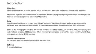
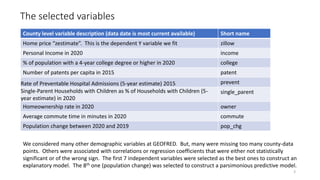
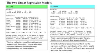
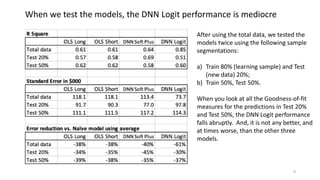
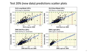
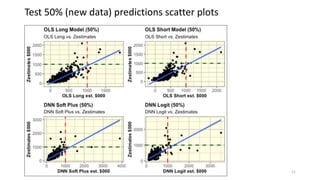
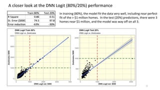
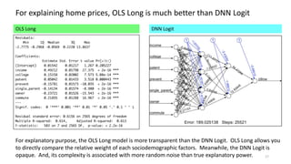
The document discusses the modeling of county-level housing prices using various demographic variables and compares four different models, including linear regression and deep neural networks (DNNs). It concludes that while the DNN logit model initially appears superior in training, it suffers from overfitting and performs poorly in prediction compared to simpler OLS models. Ultimately, OLS models are deemed more reliable for predicting and explaining home prices due to their transparency and reduced overfitting issues.

1. Housing Price Models
Gaetan Lion, May 23, 2022

2. Introduction
Objectives
My first objective was to model housing prices at the county level using explanatory demographic variables.
My second objective was to benchmark four different models varying in complexity from simple linear regressions
to more complex Deep Neural Network (DNN) models.
Data
I used county level home price data from Zillow (“zestimates”) and I used, tested, and selected demographic
variables from the GEOFRED data in order to estimate the mentioned county-level home price zestimates.
Some of the demographic variables at GEOFRED had data on up to close to 3,150 counties. The Zillow county level
data had data on about 2,850 counties. When eliminating missing data on any of the tested variables, I ended up
with a data set of over 2,500 counties.
Variable transformation
All variables are standardized so as to be on the same scale.
Software
R neuralnet package
2

3. The selected variables
3
County level variable description (data date is most current available) Short name
Home price “zestimate”. This is the dependent Y variable we fit zillow
Personal Income in 2020 income
% of population with a 4-year college degree or higher in 2020 college
Number of patents per capita in 2015 patent
Rate of Preventable Hospital Admissions (5-year estimate) 2015 prevent
Single-Parent Households with Children as % of Households with Children (5-
year estimate) in 2020
single_parent
Homeownership rate in 2020 owner
Average commute time in minutes in 2020 commute
Population change between 2020 and 2019 pop_chg
We considered many other demographic variables at GEOFRED. But, many were missing too many county-data
points. Others were associated with correlations or regression coefficients that were either not statistically
significant or of the wrong sign. The first 7 independent variables were selected as the best ones to construct an
explanatory model. The 8th one (population change) was selected to construct a parsimonious predictive model.

4. 4
The two Linear Regression Models
OLS Long OLS Short
This is an explanatory model that captures many
socioeconomic dimensions : income, education,
innovation, behavior, single motherhood,
homeownership, and commute time.
This is a parsimonious model that generates the same
Goodness-of-fit with only 3 variables instead of 7.
Remember all the variables are standardized. So, the
regression coefficients are indicative of the relative weight
of each variable. The derived coefficients were associated
with using the entire data set.

5. 5
The two Deep Neural Network Models
DNN Soft Plus. 2 hidden layers (3, 2) DNN Logit. 2 hidden layers (4, 2)
The DNN Soft Plus uses a more advanced smooth
Rectified Linear Unit activation function called Soft
Plus (See Appendix section). It is associated with
two hidden layers. The first one with 3 neurons,
and the second one with 2 neurons.
This DNN Logit uses an older activation function:
Sigmoid. The latter is a Logit Regression. This model
structure had no problem converging towards a
solution. However, the Sigmoid activation function is
associated with coefficient compression issue when
using more than one hidden layer (See Appendix).

6. 6
DNN Soft Plus Convergence Issue
DNN Soft Plus. 2 hidden layers (3, 2)
DNN Logit. 2 hidden layers (4, 2)
For the DNN Soft Plus model to converge towards a solution,
we had to prune down the first layer from 4 neurons down
to 3. And, we also had to increase the error threshold for
the partial derivatives from 0.1 for the DNN Logit to 0.3 for the DNN Soft Plus model. As a result, when using the
whole data, the DNN Soft Plus error at 447.5 is more than twice as large as for DNN Logit (189). And, the DNN
Soft Plus needed 63% more steps (41,652 vs 25,521) to converge towards a solution.

7. 7
Fitting the entire data set. The DNN Logit model is the clear winner
The scatter plots top right
hand quadrant defined by the
red and green dashed lines
show the homes with
zestimates > $1 million.
The DNN Logit models fit the
zestimates > $1 million
perfectly. The other three
models do not fit well the > $1
million data points.

8. 8
Fitting the entire data set. The DNN Logit model is the clear winner. Part II
On all Goodness-of-fit measure, the DNN Logit model is way superior to the other three. It was expected since the DNN
Logit could exploit non-linear relationships that the OLS models could not. Also, the DNN Logit model converged towards
a solution with a much lower error than the DNN Soft Plus.
Technical notes:
When calculating the standard error, we assumed for simplicity, that each model had the same degree of freedom of 1.
Given the large sample (> 2,500), this assumption did not affect the result much. The standard error was transformed
from standardized units to nominal home values in $000.
The error reduction is calculated by comparing the standard error of the model with the standard deviation of the
dependent variable (which would be the standard error of a naïve model using the average of Y as a single estimate.
Let’s say a model has a standard error of 5, and Y has a standard deviation of 10. The error reduction = 5/10 -1 = - 50%.

9. 9
When we test the models, the DNN Logit performance is mediocre
After using the total data, we tested the
models twice using the following sample
segmentations:
a) Train 80% (learning sample) and Test
(new data) 20%;
b) Train 50%, Test 50%.
When you look at all the Goodness-of-fit
measures for the predictions in Test 20%
and Test 50%, the DNN Logit performance
falls abruptly. And, it is not any better, and
at times worse, than the other three
models.

10. 10
Test 20% (new data) predictions scatter plots

11. 11
Test 50% (new data) predictions scatter plots

12. 12
A closer look at the DNN Logit (80%/20%) performance
In training (80%), the model fit the data very well, including near perfect
fit of the > $1 million homes. In the test (20%) predictions, there were 3
homes near $1 million, and the model was way off on all 3.

13. 13
A closer look at the DNN Logit (50%/50%) performance
Same situation as for the 80/20 testing. The perfect fit in training on
the homes > $1 million did not help in predicting in testing similar
homes > $1 million.

14. 14
A perfect representation of overfitting … the DNN Logit model
During training, the DNN Logit model gives you the illusion that it has captured very precise non linear
relationships to perfectly fit the homes > $1 million (left graph). But, in the testing (right graph) this same
model is unable to predict similar homes > $1 million. Thus, during the training the DNN Logit model
really fit random
noise much more
than any true non
linear
relationships.

15. 15
Overfitness within OLS vs DNN models
The DNN Logit model has a much superior fit in training or when fitting using the whole data. But, is
less accurate in prediction. Again, that is a classic definition of model overfitting. It overfits on random
outliers using non linear DNN fitting capabilities that do not reflect true non linear relationships.
The OLS models have reasonably equal performance in fitting actual data vs. in predicting new data
(test). Given that, they are way less overfit than the DNN models (especially the DNN Logit one).

16. 16
For predicting home prices, OLS Short is much better than DNN Logit
OLS Short DNN Logit
With just 3 variables, the OLS Short model predicts better than the DNN Logit with 7 variables and two
hidden layers (4, 2). Also, OLS regression math is fast and closed form. DNN math is just the opposite.

17. 17
For explaining home prices, OLS Long is much better than DNN Logit
OLS Long DNN Logit
For explanatory purpose, the OLS Long model is more transparent than the DNN Logit. OLS Long allows you
to directly compare the relative weight of each sociodemographic factors. Meanwhile, the DNN Logit is
opaque. And, its complexity is associated with more random noise than true explanatory power.

18. 18
We did not speak much about the DNN Soft Plus model …
… that’s because it was neither here nor there. It pretty much replicated the
performance of the OLS models. And, it did that in the most burdensome and opaque
way possible (these characteristics are rather typical of DNNs).
In view of the above, right off the bat you would not choose it over the OLS models. By
contrast, the DNN Logit model seemed most promising in training, as it was far superior
to the other models. But, when conducting testing, it turned out that the DNN Logit was
just way overfit.

19. 19
A quick word about DNNs Activation Functions
Appendix Section

20. 20
Common DNNs Activation Functions
Until around 2017, the preferred DNN activation function was the Sigmoid or Logistic one as it had an implicit
probabilistic weight to a Yes or No loading of a node or neuron. However, soon after the Rectified Linear Unit (ReLU)
became the preferred DNN activation function. We will advance that SoftPlus, also called smooth ReLU, should be
considered a superior alternative to ReLU. See further explanation on the next slide.

21. 21
The Sigmoid or Logistic Activation Function
There is nothing wrong with the Sigmoid function per se. The problem occurs when you take the first derivative of this
function. And, it compresses the range of the values by 50% (from 0 to 1, to 0 to 0.5 for the first iteration). In iterative DNN
models, the output of one hidden layer becomes the input for the sequential layer. And, this 50% compression from one
layer to the next can generate values that converge close to zero. This problem is called the “vanishing gradient descent.”
We will see that in our situation, this problem is not material.

22. 22
ReLU and smooth ReLU or SoftPlus Activation Functions
SoftPlus appears superior to ReLu because it captures the weights of many more neurons’ features, as it does not zero
out any such features with an input value < 0. Also, it generates a continuous set of derivatives values ranging from 0 to
1. Instead, ReLu derivatives values are limited to a binomial outcome (0, 1).